| Issue |
A&A
Volume 616, August 2018
|
|
|---|---|---|
| Article Number | A171 | |
| Number of page(s) | 20 | |
| Section | Extragalactic astronomy | |
| DOI | https://doi.org/10.1051/0004-6361/201833089 | |
| Published online | 31 August 2018 | |
Spatially resolved cold molecular outflows in ULIRGs★
1
Department of Physics, University of Oxford,
Keble Road,
Oxford
OX1 3RH,
UK
e-mail: This email address is being protected from spambots. You need JavaScript enabled to view it.
2
Centro de Astrobiología (CSIC/INTA), Ctra de Torrejón a Ajalvir,
km 4,
28850
Torrejón de Ardoz,
Madrid,
Spain
3
Observatorio Astronómico Nacional (OAN-IGN)-Observatorio de Madrid,
Alfonso XII, 3,
28014
Madrid,
Spain
4
LERMA, Observatoire de Paris, PSL Research University, Collège de France, CNRS, Sorbonne University, UPMC,
Paris,
France
5
National Radio Astronomy Observatory,
520 Edgemont Road,
Charlottesville,
VA 22903,
USA
6
Department of Space, Earth and Environment, Onsala Space Observatory, Chalmers University of Technology,
439 92
Onsala,
Sweden
7
Max-Planck-Institut für Radioastronomie,
Auf dem Hügel 69,
53121
Bonn,
Germany
8
Astronomy Department, King Abdulaziz University,
PO Box 80203,
Jeddah
21589,
Saudi Arabia
9
Leiden Observatory, Leiden University,
PO Box 9513,
2300 RA
Leiden,
The Netherlands
Received:
23
March
2018
Accepted:
7
May
2018
Abstract
We present new CO(2–1) observations of three low-z (d ~350 Mpc) ultra-luminous infrared galaxy (ULIRG) systems (six nuclei) observed with the Atacama large millimeter/submillimeter array (ALMA) at high spatial resolution (~500 pc). We detect massive cold molecular gas outflows in five out of six nuclei (Mout ~ (0.3−5) × 108 M⊙). These outflows are spatially resolved with deprojected effective radii between 250 pc and 1 kpc although high-velocity molecular gas is detected up to Rmax ~ 0.5−1.8 kpc (1–6 kpc deprojected). The mass outflow rates are 12–400 M⊙ yr−1 and the inclination corrected average velocity of the outflowing gas is 350–550 km s−1 (vmax = 500−900 km s−1). The origin of these outflows can be explained by the strong nuclear starbursts although the contribution of an obscured active galactic nucleus cannot be completely ruled out. The position angle (PA) of the outflowing gas along the kinematic minor axis of the nuclear molecular disk suggests that the outflow axis is perpendicular to the disk for three of these outflows. Only in one case is the outflow PA clearly not along the kinematic minor axis, which might indicate a different outflow geometry. The outflow depletion times are 15–80 Myr. These are comparable to, although slightly shorter than, the star-formation (SF) depletion times (30–80 Myr). However, we estimate that only 15–30% of the outflowing molecular gas will escape the gravitational potential of the nucleus. The majority of the outflowing gas will return to the disk after 5–10 Myr and become available to form new stars. Therefore, these outflows will not likely completely quench the nuclear starbursts. These star-forming powered molecular outflows would be consistent with being driven by radiation pressure from young stars (i.e., momentum-driven) only if the coupling between radiation and dust increases with increasing SF rates. This can be achieved if the dust optical depth is higher in objects with higher SF. This is the case in at least one of the studied objects. Alternatively, if the outflows are mainly driven by supernovae (SNe), the coupling efficiency between the interstellar medium and SNe must increase with increasing SF levels. The relatively small sizes (<1 kpc) and dynamical times (<3 Myr) of the cold molecular outflows suggests that molecular gas cannot survive longer in the outflow environment or that it cannot form efficiently beyond these distances or times. In addition, the ionized and hot molecular phases have been detected for several of these outflows, so this suggests that outflowing gas can experience phase changes and indicates that the outflowing gas is intrinsically multiphase, likely sharing similar kinematics, but different mass and, therefore, different energy and momentum contributions.
Key words: galaxies: active / galaxies: ISM / galaxies: kinematics and dynamics / galaxies: nuclei / galaxies: starburst
The reduced images and datacubes are only available at the CDS via anonymous ftp to cdsarc.u-strasbg.fr (130.79.128.5) or via http://cdsarc.u-strasbg.fr/viz-bin/qcat?J/A+A/616/A171
© ESO 2018
1 Introduction
Negative feedback from active galactic nuclei (AGN) and starbursts plays a fundamental role in the evolution of galaxies according to theoretical models and numerical simulations (e.g., Narayanan et al. 2011; Scannapieco et al. 2012; Hopkins et al. 2012; Nelson et al. 2015; Schaye et al. 2015). This feedback occurs through the injection of material, energy, and momentum into the interstellar medium (ISM) and gives rise to massive gas outflows and regulates the growth of the stellar mass and black-hole accretion.
Such energetic and massive outflows have been detected in galaxies at low and high redshift. In particular, they have been detected in ultra-luminous infrared galaxies (ULIRGs; LIR > 1012 L⊙) in their atomic ionized (e.g., Westmoquette et al. 2012; Arribas et al. 2014), atomic neutral (e.g., Rupke et al. 2005; Cazzoli et al. 2016), and cold molecular (e.g., Fischer et al. 2010; Feruglio et al. 2010; Sturm et al. 2011; Cicone et al. 2014) phases. Local ULIRGs are major gas-rich mergers mainly powered by star formation (SF), although AGN accounting for a significant fraction of the total infrared (IR) luminosity (10− 60%) are usually detected too (Farrah et al. 2003; Nardini et al. 2010). Since local ULIRGs are the hosts of the most extreme starbursts in the local Universe with star-formation rates (SFR) greater than ~150 M⊙ yr−1, based on their IR luminosities (Kennicutt & Evans 2012), they are adequate objects to study the negative feedback from both AGN and SF. In this paper, we focus on the molecular phase of these outflows. This phase includes molecular gas with a wide range of temperatures. The hot (T > 1500 K) and the warm (T > 200 K) molecular phases can be observed using the near-IR ro-vibrational H2 transitions (e.g., Emonts et al. 2014, 2017; Dasyra et al. 2015) and the mid-IR rotational H2 transitions (e.g., Hill & Zakamska 2014). However, it is thought that the energy and mass of these outflows are dominated by the cold molecular phase (e.g., Feruglio et al. 2010; Cicone et al. 2014; Saito et al. 2018), although some observations and models seem to contradict this view (e.g., Hopkins et al. 2012; Dasyra et al. 2016). The cold molecular phase has been detected using multiple CO transitions (e.g., Feruglio et al. 2010; Chung et al. 2011; Cicone et al. 2014; García-Burillo et al. 2015; Pereira-Santaella et al. 2016), HCN transitions (e.g., Aalto et al. 2012; Walter et al. 2017; Barcos-Muñoz et al. 2018), and far-IR OH absorption (Fischer et al. 2010; Sturm et al. 2011; Spoon et al. 2013; González-Alfonso et al. 2017). All these observations have revealed that cold molecular outflows are common in ULIRGs and that they can be massive enough to play a relevant role in the regulation of the SF in their host galaxies.
Knowing the distribution of the outflowing gas is important to derive accurate outflow properties, like the outflow mass, energy, and momentum rates, which are key to determine the impact of these outflows onto their host galaxies. However, spatially resolved observations of outflows in ULIRGs are still limited to a few sources (e.g., García-Burillo et al. 2015; Veilleux et al. 2017; Barcos-Muñoz et al. 2018; Saito et al. 2018). Here, we present new high angular resolution (~ 0.′′3−0.′′4) Atacama large millimeter/submillimeter array (ALMA) observations of the CO(2–1) transition in three low-z ULIRGs where the cold molecular outflow phase is spatially resolved on scales of ~500 pc. This provides a direct measurement of the outflow size and therefore allows us to derive more accurately the outflow properties.
This paper is organized as follows: the sample and the ALMA observations are described in Sect. 2. In Sect. 3, we analyze the 248 GHz continuum and CO(2–1) emissions and measure the outflow properties in these systems. The energy source of the outflows, as well as their impact, launching mechanism, and multi-phase structure are discussed in Sect. 4. Finally, in Sect. 5, we summarize the main results of the paper. Throughout this article we assume the following cosmology: H0 = 70 km s−1 Mpc−1, Ωm = 0.3, and ΩΛ = 0.7.
2 Observations and data reduction
2.1 Sample of ULIRGs
In this paper, we study three low-z (d ~ 350 Mpc) ULIRGs (six individual nuclei) with logLIR∕L⊙ = 12.0−12.3 (see Table 1) based on their mid- and far-IR spectral energy distribution modeling (Sect. 3.4.1). These three ULIRG systems seem to be in a similar dynamical state. They were classified as type III by Veilleux et al. (2002), which corresponds to a pre-merger stage characterized by two identifiable nuclei with well defined tidal tails and bridges. They also belong to the subclass of “close binary” (i.e., “b”) as the projected separation of their nuclei is smaller than 10 kpc.
The nuclei of these galaxies are classified as low ionization nuclear emission-line regions (LINER; IRAS 12112+0305 and IRAS 14348−1447; e.g., Colina et al. 2000; Evans et al. 2002)or H II (IRAS 22491−1808; e.g., Veilleux et al. 1999) and in all systems a weak AGN contribution (10− 15%) is detected in their mid-IR Spitzer spectra (Veilleux et al. 2009). For IRAS 14348−1447, high-angular-resolution mid-IR imaging suggests that the AGN is located in the southwest nucleus (Alonso-Herrero et al. 2016). For IRAS 12112+0305 and IRAS 22491−1808, we assume that the AGN is at the brightest nucleus in the radio/sub-mm continuum, that is, IRAS 12112+0305 NE and IRAS 22491−1808 E (see below). In addition, vibrationally excited HCN J = 4−3 emission is detected in IRAS 12112+0305 NE and IRAS 22491−1808 E, which can be a signature of hot dust heated by an AGN (Imanishi et al. 2016, 2018). In addition, these three ULIRGs belong to a representative sample of local ULIRGs studied by García-Marín et al. (2009a,b), Arribas et al. (2014), and Piqueras López et al. (2012) using optical and near-IR integral field spectroscopy.
Sample of local ULIRGs.
2.2 ALMA data
We obtained Band 6 ALMA CO(2–1) 230.5 GHz and continuum observations for these three local ULIRGs (see Table 1) as part of the ALMA projects 2015.1.00263.S and 2016.1.00170.S (PI: Pereira-Santaella). The observations were carried out between June 2016 and May 2017. The total on-source integration times per source were ~30−40 min split into two scheduling blocks. The baseline lengths range between 15 and 1100 m providing a synthesized beam full width at half maximum (FWHM) of ~ 0.′′3−0.′′4 (400−500 pc at the distance of these ULIRGs). Details on the observations for each source are listed in Table 2.
Two spectral windows of 1.875 GHz bandwidth (0.976 MHz ≡ ~1.3 km s−1 channels) were centered at the sky frequency of the 12CO(2–1) and CS(5–4) transitions (see Table 2). In addition, a continuum spectral window was set at ~248 GHz (~1.2 mm). In this paper, we analyze the CO(2–1) and continuum spectral windows; the CS(5–4) data will be presented in a future paper.
The data were calibrated using the ALMA reduction software Common Astronomy Software Applications (CASA v4.7; McMullin et al. 2007). The amplitude calibrators for each scheduling block are listed in Table 2. For the CO(2–1) spectral window, a constant continuum level was estimated using the line free channels and then subtracted in the uv-plane. For the image cleaning, we used the Briggs weighting with a robustness parameter of 0.5 (Briggs 1995). The synthesized beam (~ 0.′′3−0.′′4) and maximum recoverable scale (~ 4′′) are presented in Table 2 for each observation. To our knowledge, there are no single-dish CO(2–1) fluxes published for these ULIRGs so it is not straightforward to estimate if we filter part of the extended emission. However, the bulk of the CO(2–1) emission of these systems is relatively compact (see Sect. 3.1.1 and Figs. B.1–B.3 in Appendix B), so we expect to recover most of the CO(2–1) emission with these array configurations. The final datacubes have 300 × 300 spatial pixels of 0.′′ 08 and 220 spectral channels of 7.81 MHz (~10 km s−1). For the CO(2–1) cubes, the 1σ sensitivity is ~ 310−450μJy beam−1 per channel and ~ 30−45μJy beam−1 for the continuum images. A primary beam correction (FWHM ~20′′) was applied to the data.
ALMA observation log.
2.3 Near-IR HST imaging
We downloaded the near-IR Hubble space telescope/Near Infrared Camera and Multi-Object Spectrometer (HST/NICMOS) F160W (λc = 1.60 μm, FWHM = 0.34μm) and F222M (λc = 2.21 μm, FWHM = 0.15μm) reduced images from the Mikulski Archive for Space Telescopes (MAST). The angular resolutions of these images are 0.′′ 14 and 0.′′ 20 for the F160W and F222M filters, respectively, which is slightly better than the resolution of the ALMA data. The ALMA and HST images were aligned using the positions of the nuclei in the 248 GHz and F222M images. The F222M filter was used because it is less affected by dust obscuration than F160W. If the 2.2 μm near-IR and 248 GHz continua have similar spatial distributions in these ULIRGs, the uncertainty of the image alignment is about 0.′′08 (~120 pc) limited by the centroid accuracy in the HST data.
3 Data analysis
3.1 Morphology
In Figs. 1–3, we present the CO(2–1) and 248 GHz continuum emission maps of the three ULIRGs.
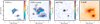 |
Fig. 1 ALMA and HST maps for IRAS 12112+0305. The first and second panels are the CO(2–1) integrated flux and peak intensity for ~10 km s−1 channels, respectively. The contour levels in the second panel correspond to (6, 18, 54, 162, 484) × σ, where σ is the line sensitivity (Table 2). The third panel is the ALMA 248 GHz continuum. The contours in this panel are (3, 27, 81) × σ where σ is the continuum sensitivity (Table 2). The fourth panel shows the near-IR HST/NICMOS F160W map with the CO(2–1) peak contours. The position of the two nuclei is marked with a cross in all the panels. The red hatched ellipse represents the FWHM and PA of the ALMA beam (Table 2). |
3.1.1 Molecular gas
The molecular gas traced by the CO(2–1) transition, which is dominated by the emission from the central ~ 1−2 kpc, has an irregular morphology with multiple large-scale tidal tails (up to ~10 kpc) and isolated clumps. These characteristics are very likely connected to the ongoing galaxy interactions taking place in these systems. Similar tidal tails are observed in the stellar component in the near-IR HST/NICMOS NIC2 images (right- hand panel of Figs. 1–3). However, there are noticeable offsets, ~1−2 kpc, between the position of these stellar and molecular tidal tails.
To measure the total CO(2–1) emission of each system, we first defined the extent of this emission by selecting all the contiguous pixels where the CO(2–1) line peak is above 6σ (see second panel of Figs. 1–3). Then, we integrated the line flux in this area. The resulting flux densities are presented in Table 3. The flux strongly peaks at the nuclei of these objects, so we calculate an effective radius based on the area, A, which encloses half of the total CO(2–1) emission as 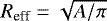 . This Reff provides a better estimate of the actual size of the CO(2–1) emission. For these galaxies, the effective radius varies between 400 pc and 1kpc (see Table 3).
Both in IRAS 12112 and IRAS 22491, the CO(2–1) emission is completely dominated by one of the galaxies that produces 80 and 90%, respectively, of the total flux of the merging system. In IRAS 14348, the CO(2–1) emission is also dominated by one of the nuclei (SW), but this one is only two times brighter than the NE nucleus.
Integrated CO(2–1) emission.
3.1.2 248 GHz continuum
Except for the western nucleus of IRAS 22491, which is not seen at 248 GHz, the remaining nuclei are clearly detected in both the CO(2–1) and continuum images. In all the cases, the 248 GHz continuum emission is produced by a relatively compact source. To accurately measure the continuum properties, we used the UVMULTIFIT library (Martí-Vidal et al. 2014) within CASA. This library can simultaneously fit various models to the visibility data. First, we tried a two-dimensional (2D) circular Gaussian model, which provided a good fit for all the sources except two (I12112 NE and I22491 E). For these two sources, we added a delta function with the same center as a second component to account for the unresolved continuum emission. This second unresolved component represents 70− 80% of the total continuum emission in these objects. The results of the fits are presented in Table 4 and the center coordinates listed in Table 1 (see also Appendix A).
The resolved continuum emission (2D circular Gaussian component of the model) has a FWHM between 260 and 1000 pc, which is more compact than the CO(2–1) emission. For comparison, the CO(2–1) effective radius is three to six times larger than the FWHM/2 of this 2D Gaussian component. Only in I22491 E, both have similar sizes, although, in this galaxy, the continuum emission is dominated by the unresolved component. Therefore, in all these ULIRGs, the 248 GHz continuum emission is considerably more compact than the molecular CO(2–1) emission. This is similar to what is observed in other local luminous IR galaxies (LIRGs) and ULIRGs (e.g., Wilson et al. 2008; Sakamoto et al. 2014; Saito et al. 2017).
In IRAS 12112 and IRAS 22491, the continuum emission is dominated by the same nucleus that dominates the CO(2–1) emission (see Sect. 3.1.1). The fractions of the 248 GHz continuum produced by these dominant nuclei are 90 and >95%, respectively, which are slightly higher than their contributions to the total CO(2–1) luminosity of their systems (80 and 90%, respectively). In IRAS 14348, the SW nucleus produces 60% of the continuum emission and the NW produces the remaining 40%. These fractions are similar to those of the CO(2–1) produced in each nucleus (65 and 35%, respectively).
The 248 GHz continuum emission is possibly produced by a combination of thermal dust continuum, free–free radio continuum, and synchrotron emission. The latter can be dominant at this frequency in the case of AGN, and, as discussed in Sect. 2.1, AGN emission is detected in the three ULIRGs. To determine the non-thermal contribution to the measured 248 GHz fluxes, we use the available interferometric radio (1.49 and 8.44 GHz) observations for these systems (Condon et al. 1990, 1991). The position of the 248 GHz continuum sources is compatible with the location of the 1.49 and 8.44 GHz radio continuum emission within 0.′′15 (~half of the beam FWHM). Therefore, we assume that the radio and the 248 GHz emissions are produced in the same regions. We also note that the western nucleus of IRAS 22491 is undetected as well at radio wavelengths. For the rest of the sources, we fit a power law to the 1.49 and 8.44 GHz fluxes and obtain spectral indexes between 0.42 and 0.72. Then, we use these spectral indexes to extrapolate the non-thermal emission at 248 GHz. On average, this represents 20% of the 248 GHz emission for these ULIRGs (see Table 4), with a minimum (maximum) contribution of 14% (43%). Therefore, most of the 248 GHz emission is likely due to thermal dust emission and free–free radio continuum produced in the compact nuclear region.
ALMA continuum models.
3.2 Molecular gas kinematics
3.2.1 Global kinematics
In Fig. 4, we show the first and second moments of the CO(2–1) emission for each galaxy of the three ULIRG systems andindicate the outflow axis (dotted line) and the kinematic major axis of the nuclear disk (dashed line) defined in Sect. 3.2 (see Fig. 5). The first moment maps indicate a complex velocity field, although a rotating disk patternis present in all the systems. The second moment maps show that the velocity dispersion maximum (120−170 km s−1) is almost coincident with the location of the nucleus and that it is enhanced more or less along the molecular outflow axis (dotted line). The latter is expected since the high-velocity outflowing gas produces broad wings in the CO(2–1) line profile, which enhances the observed second moment.
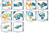 |
Fig. 4 For each galaxy of the ULIRG systems, the left- and right-hand panels show the first and second moments of the CO(2–1) emission, respectively. The spacings between the contour levels in the first and second moment maps are 100 and 25 km s−1, respectively.For the first moment maps, the velocities are relative to the systemic velocity (see Table 1). The red box in this panel indicates the field of view presented in Fig. 5 for each object. The dashed and dotted lines mark the kinematic major axis and the outflow axis, respectively, defined in Sect. 3.2 (see also Fig. 5). The black cross marks the position of the 248 GHz continuum peak. The red hatched ellipse shows the beam FWHM and PA. |
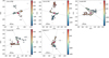 |
Fig. 5 Centroid of the CO(2–1) emission measured in each ~10 km s−1 velocity channel. The color of the points indicates the CO(2–1) velocity with respect to the systemic velocity not corrected for inclination. The rose diamond marks the position of the 248 GHz continuum peak. The dashed line is the linear fit to the low velocity gas and corresponds to the kinematic major axis of the rotating disk. The dotted line is the linear fit to the high-velocity red- and blue-shifted gas, which traces the projection of the outflow axis in the sky. The error bars in each point indicate the statistical uncertainty in the centroid position. The gray error bars represent the astrometric accuracy of these observations for channels with S∕N > 10 (see Sect. 3.2). |
3.2.2 Nuclear disks and molecular outflows
Similar to García-Burillo et al. (2015), we derive the centroid of the CO(2–1) emission in each velocity channel to study the nuclear gas kinematics and identify high-velocity gas decoupled from the rotating disks. The results are presented in Fig. 5. Thanks to the high signal-to-noise ratio (S/N) of the data, we are able to determine the centroid positions with statistical uncertainties <10 mas for most of the channels. The astrometric accuracy for the frequency and array configuration of these observations is ~25 mas for channelswith a S/N higher than 10. For channels with a S/N of approximately 3, this accuracy is reduced to ~80 mas1. Therefore, the shifts of the centroid positions shown in Fig. 5 are expected to be real.
For all the objects, the low-velocity emission centroids follow a straight line. This is consistent with the emission from a rotating disk that is not completely resolved. The direction of this line traces the position angle (PA) of the kinematic major axis of the rotating disk. Therefore, we did a linear fit to these points and derived the disk PA (Table 5). Also, using these fits, we determined the systemic velocity as the velocity of the point along the major axis closest to the continuum peak (Table 1).
By contrast, the centroids of the high-velocity gas do not lie on the kinematic major axis and they cluster at two positions, one for the red-shifted and the other for the blue-shifted gas. These two positions are approximately symmetric with respect to the nucleus. This is strong evidence of the decoupling of the high-velocity gas from the global disk rotation and, as we discuss in Sect. 3.3, this is compatible with the expected gas distribution of a massive molecular outflow originating at the nucleus. Alternatively, if we assume a coplanar geometry for the high-velocity gas, these PA twists could be explained by a strong nuclear bar-like structure. However, because of the extremely high radial velocities implied by this geometry, up to 400 km s−1, in the following, we only discuss the out-of-plane outflow possibility.
The inclination of the disks is an important parameter to derive accurate outflow properties. It is commonly derived from the ratio between the photometric major and minor axes assuming that the galaxy is circular. However, in these merger systems, it is not obvious how to define these axes and also the circular morphology assumption might be incorrect. Therefore, we use an alternative approach based on the kinematic properties of the nuclear disks to estimate the inclination. First, we extract the rotation curve along the kinematic major axis, and fit an arctan model (e.g., Courteau 1997) to determine the curve semi-amplitude, v (Fig. 6 and Table 5). Then, we measure the velocity dispersion, σ, of the nuclear region (1–2 kpc) and calculate the observed dynamical ratio v∕σ. García-Marín et al. (2006) and Bellocchi et al. (2013) measured the v∕σ ratios in a sample of 25 ULIRGs (34 individual galaxies) with Hα integral field spectroscopy. Assuming a mean inclination of 57° (sin i = 0.79; see Law et al. 2009), we can correct their v values for inclination and determine an intrinsic v∕σ ratio of 1.5 ± 0.6 for ULIRGs. Then, we compare the observed dynamical ratios in each galaxy with this intrinsic ratio to estimate their inclinations (15−40°).
Nuclear molecular emission.
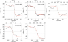 |
Fig. 6 Rotation curves of the ULIRGs extracted along the kinematic major axis. The red line shows the best fit arctan model to the data. The fit results are presented in Table 5. |
3.3 Properties of the molecular outflows
3.3.1 Observed properties: PA, size, flux, and velocity
In the previous section, we presented the detection of high-velocity gas in five out of six ULIRG nuclei, which is compatible with the presenceof massive molecular outflows. But depending on which side of the rotating disk is closest to us, this high-velocity gas can be interpreted as an inflow or as an outflow. To investigate this, we plot the morphological features (spiral arms or tidal tails) we identified in the CO(2–1) channel maps (panel d of Figs. 7–11 and Appendix B). Then, in panel e of these figures, we plot the identified morphological features over the velocity fields and, assuming that these features are trailing, we can determine the near- and far-side of the rotating disk. For all the galaxies where the high-velocity emission is spatially resolved, the blue-shifted high-velocity emission appears on the far side of the disk and the red-shifted emission on the near side. This is a clear signature of outflowing gas.
In addition, we can measure the PA of these outflows by fitting the position of the red and blue centroid clusters with a straight line (Fig. 5 and Table 5). We calculated the difference between the PA of the high-velocity gas and that of the kinematic major axis of the disk (Table 5) and found values around 90° for three cases. This PA difference is the expected value for an outflow perpendicular to the rotating disk. For IRAS 14348 SW, the PA difference is ~126 ± 8°, which suggests a different outflow orientation. Finally, the outflow PA of IRAS 22491 E seems to deviate from a perpendicular orientation although with less significance due to the large uncertainty (~120 ± 20°).
In panel a of Figs. 7–11, we show the spatial distribution of the high-velocity gas emission. This emission is spatially resolved, except for IRAS 22491 E, and reaches projected distances, Rmax, up to 0.′′ 4–1.′′2 (0.5−1.8 kpc; see Table 6) from the nucleus. We note that these sizes are a factor of three to five larger than the sizes derived from the separation between the blue- and red-shifted emission centroids (Rc). In the following, we use the Rc as the outflow size because, as a flux-weighted estimate of the outflow size, it is a better estimate of the extent of the region where most of the outflowing molecular gas is located. On the other hand, Rmax is dominated by the faint CO(2–1) emission at larger radii and it is also likely dependent on the sensitivity of the observations.
The outflows are clearly spatially resolved (2 × Rmax > FWHM of the beam). However, the angular resolution is not high enough to allow us to measure the outflow properties as a function of radius. For this reason, we only consider the integrated outflow emission and measure a total outflow flux. To do so, we extracted the spectrum of the regions where high-velocity gas is detected (panel b of Figs. 7–11). We fit a two-Gaussian model to the CO(2–1) line profile. This model reproduces well the core of the observed line profile. The residual blue and red wings (i.e., the outflow emission) are shown in panel c of Figs. 7–11 for each galaxy. From these spectra, we also estimate the flux-weighted average velocity of the outflowing gas (320−460 km s−1) and the maximum velocity at which we detect CO(2–1) emission (400−800 km s−1). The total CO(2–1) flux, as well as the flux in the high-velocity wings, are presented in Table 6.
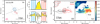 |
Fig. 7 Blue and red contours in panel a represent the integrated blue- and red-shifted high-velocity CO(2–1) emission, respectively.The specific velocity range is listed in Table 6. The lowest contour corresponds to the 3σ level. The next contour levels are (0.5, 0.9) × the peak of the high-velocity emission when these are above the 3σ level. For I12112 SW, σ = 30 mJy km s−1 beam−1 and the red and blue peaks are at 110 and 240 mJy km s−1 beam−1, respectively. The dotted and the dashed lines are the outflow axis and the kinematic major axis, respectively (see Table 5). The red hatched ellipse represents the beam FWHM and PA. The dashed circle indicates the region from which the nuclear spectrum was extracted. Panel b: nuclear spectrum in yellow and the best-fit model in gray. Panel c: difference between the observed spectrum and the best-fit model. The shaded blue and red velocity ranges in these panels correspond to the velocity ranges used for the contours of panel a. The gray line in panel c marks the 3σ noise level per channel. Panel d: CO(2–1) emission at the velocities indicated by the numbers at the top-right corner of the panel as black and red contours, respectively. The black and red double lines trace the morphological features (spiral arms, tidal tails) observed at those velocities. Panel e: CO(2–1) mean velocity field (same as in Fig. 4). The black dashed line is the kinematic major axis and the gray dot-dashed line is the kinematic minor axis. The far and near sides of the rotating disk are indicated, assuming that the observed morphological features are trailing. |
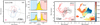 |
Fig. 8 Same as Fig. 7 but for I12112 NE. In panel a, σ = 45 mJy km s−1 beam−1 and the red and blue peaks are at 2.4 and 2.9 Jy km s−1 beam−1, respectively. |
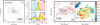 |
Fig. 9 Same as Fig. 7 but for I14348 SW. In panel a, σ = 46 mJy km s−1 beam−1 and the red and blue peaks are at 1.4 and 1.0 Jy km s−1 beam−1, respectively. |
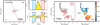 |
Fig. 10 Same as Fig. 7 but for I14348 NE. In panel a, σ = 32 mJy km s−1 beam−1 and the red and blue peaks are at 0.74 and 0.56 Jy km s−1 beam−1, respectively. |
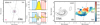 |
Fig. 11 Same as Fig. 7 but for I22491 E. In panel a, σ = 43 mJy km s−1 beam−1 and the red and blue peaks are at 1.1 and 2.2 Jy km s−1 beam−1, respectively. |
3.3.2 Derived properties
In Table 7, we present the derived properties for these outflows based on the observations and assuming that they are perpendicular to the rotating disk. The latter is consistent with the ~ 90° PA difference between the kinematic major axis and the outflow axis measured in three of the galaxies. For the other two cases (PA difference ~ 120°), this assumption might introduce a factor of approximately two uncertainty into the derived outflow rates.
To convert the CO(2–1) fluxes into molecular masses, we assume a ULIRG-like αCO conversion factor of 0.78 M⊙ (K km s−1 pc−2)−1 and a ratiobetween the CO(2–1) and CO(1–0) transitions, r21, of 0.91 (Bolatto et al. 2013). The outflow velocity is corrected for the inclination by dividing by cos i, where i is the disk inclination (Table 5). Similarly, the outflow radius is corrected by dividing by sin i. The average corrected outflow velocity is ~440 km s−1 and the average deprojected radius is ~700 pc.
Using these quantities, we calculate the dynamical time as tdyn = Rout∕vout (about ~1 Myr for these outflows). Then, we estimate the outflow rate using Ṁout = Mout∕tdyn. We find Ṁout values between ~12 and ~400 M⊙ yr−1. From these estimates, we can derive the depletion time (tdep), outflow momentum rate (Ṗout), and the outflow kinetic luminosity (Lout; see, e.g., García-Burillo et al. 2015).
The uncertainties on the outflow rate, and the quantities derived from it, are dominated by the uncertainty in the value of the αCO conversion factor, which is not well established for the outflowing gas (e.g., Aalto et al. 2015) and the outflow geometry (inclination). For the conversion factor, we assume a ULIRG-likevalue (αCO = 0.78 M⊙ (K km s−1 pc−2)−1), although depending on the gas conditions, this factor can vary within 0.3 dex (e.g., Papadopoulos et al. 2012; Bolatto et al. 2013). Therefore, from the uncertainty in the inclination and the conversion factor, we assume a 0.4 dex uncertainty for these values.
Finally, in Table 8, we estimate the fraction of the outflowing gas that would escape the gravitational potential of these galaxies. We use the escape velocities at 2 kpc calculated by Emonts et al. (2017) for these systems that range from ~400 to 600 km s−1. We integrate the CO(2–1) emission with velocities higher than these escape ones (taking into account the inclination of the outflows) and obtain that 15− 30% of the high-velocity gas will escape to the intergalactic medium. The escape outflow rates are 3− 120M⊙ yr−1. However, these escape rates can be lower if the velocity of the outflowing gas is decreased due to dynamical friction.
3.4 Nuclear SFR
Measuring the SFR in these ULIRGs is important to evaluate the impact of the molecular outflows. Most of the outflowing molecular gas is concentrated in the central 1−2 kpc, so to determine the local effect of the outflows, we must compare them with the nuclear SFR. However, the nuclei of local ULIRGs are extremely obscured regions (e.g., García-Marín et al. 2009a; Piqueras López et al. 2013) and estimating their SFR is not straightforward. In this section, we use two approaches to measure the nuclear SFR using the IR luminosity and the 248 GHz continuum and the radio continuum, which should not be heavily affected by extinction.
3.4.1 IR luminosity
The total IRluminosity (LIR) is a good tracer of the SF in dusty environments such as the nuclei of ULIRGs (e.g., Kennicutt & Evans 2012). However, there are no far-IR observations with the two nuclei of the systems spatially resolved. For this reason, we first derived the integrated LIR of each system. We fit a single temperature gray body model to the 24–500 μm fluxes from Spitzer and Herschel (Piqueras López et al. 2016; Chu et al. 2017) following Pereira-Santaella et al. (2016). The resulting LIR are ~0.2 dex lower than those derived using the IRAS fluxes, but we consider these new LIR more accurate since we are using more data points that cover a wider wavelength range to fit the IR emission (seven points between 24 and 500μm vs. four pointsbetween 12 and 100μm) and also we avoid flux contamination from unrelated sources thanks to the higher angular resolution of the new data (6′′ −35′′ vs. 0.′5−2′). The LIR are listed in Table 1 and the best fits are shown in Fig. 12.
Then, we assign a fraction of LIR due to the star formation (i.e., after subtracting the AGN luminosity from Table 1) to each nucleus, which is proportional to their contribution to the total thermal continuum at 248 GHz (dust emission plus free–free radio continuum; see Table 4) of the system. By doing this, we assume that all the LIR is produced in the central 300−1000 pc, which is consistent with the compact distribution of the molecular gas around the nuclei (Sect. 3.1.1), and that the 248 GHz continuum scales with the LIR. The latter is true for the free–free radio continuum contribution at this frequency, which is proportional to the ionizing flux and, therefore, to the SFR and LIR. The dust emission at 248 GHz depends on the average dust temperature of each nucleus (fν ∕L ∝ T−3 in the Rayleigh–Jeans tail of the black body). However, given the similar temperatures we obtained for the integrated emission (T ~ 65−70 K; see Fig. 12), our assumption seems to be reasonable. Finally, we converted these nuclear IR luminosities into SFR using the Kennicutt & Evans (2012) calibration (see Table 9). The SFRs range from 13 to 180 M⊙ yr−1.
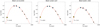 |
Fig. 12 Mid- and far-IR spectral energy distribution of the three ULIRGs. The yellow circle corresponds to the Spitzer/MIPS 24 μm flux, the blue squares to the Herschel/PACS 60, 100, and 160 μm fluxes, and the green triangles to the Herschel/SPIRE 250, 350, and 500 μm fluxes. The solid red line is the best fit to the data using a single temperature gray body. |
Nuclear CO(2–1) emission and observed outflow properties.
Derived molecular outflow properties.
3.4.2 Radio continuum
We also estimated the SFR from the non-thermal radio continuum observations of these galaxies (see Sect. 3.1.2). Using the observed 1.49 and 8.44 GHz fluxes and the derived spectral indexes, we estimated the rest-frame 1.4 GHz continuum and applied the Murphy et al. (2011) SFR calibration. Here, we ignore any contribution from an AGN to the radio emission. These objects seem to be dominated by SF and just have a small AGN contribution, but the radio emission of these AGN is uncertain.
The obtained radio SFR are listed in Table 9. These values are comparable to those obtained from the IR luminosity. The average difference between the two estimates is 0.2 dex with a maximum of 0.4 dex. Therefore, the two methods provide compatible SFR values and, in the following, we adopt the SFR(IR) with a 0.2 dex uncertainty.
Escape outflow.
Outflows and nuclear SFR.
4 Discussion
4.1 Outflow energy source
In the left panel of Fig. 13, we show the relation between the outflow rate and the nuclear SFR (i.e., the mass loading factor η). In this figure, we include local U/LIRGs with spatially resolved observations (filled symbols) as well as the lower luminosity starbursts compiled by Cicone et al. (2014)2. In total, weinclude observations for seven ULIRG nuclei, five LIRG nuclei, and four starbursts. For the two nuclei classified as AGN, we derive the nuclear SFR from their IR luminosity after subtracting the AGN contribution (see García-Burillo et al. 2015; Ohyama et al. 2015).
The five new ULIRG nuclei (encircled stars in this figure) have mass loading factors, η, ~ 0.8−2 (see Table 9). These are similar to those observed in local starburst galaxies, which are typically lower than ~ 2−3 (e.g., Bolatto et al. 2013; Cicone et al. 2014; Salak et al. 2016). This suggests that the outflows in these ULIRGs are also powered by SF.
To further investigate the energy source, in Table 9, we list the ratios between the kinetic luminosity and momentum rates of the outflows and the total energy and momentum injected by supernovae (SNe), respectively. We assume that the SNe total energy and momentum are upper limits on the energy and momentum that the starburst can inject into the outflow (independent of the launching mechanism; see Sect. 4.3). For all the galaxies, both the energy and momentum in the molecular outflowing gas are lower than those produced by SNe. Although this does not imply an SF origin, we cannot rule out the SF origin based on the energy or momentum of these outflows.
Molecular outflows from AGN usually have maximum velocities up to ~1000 km s−1 (e.g., Cicone et al. 2014; Veilleux et al. 2017), which are higher than those due to SF (a few hundreds of km s−1). We found the maximum outflow velocities in IRAS 12112 NE and IRAS 14348 SW (~ 700−800 km s−1). These are not as high as those observed in other AGN, but are 1.5−2 times higherthan in the rest of our sample and might indicate an AGN-powered outflow in these objects. However, there are molecular outflows detected in more nearby starbursts that also reach these high velocities (e.g., Sakamoto et al. 2014). Therefore, the velocities of the outflows in these ULIRGs are not high enough to claim an AGN origin.
Similarly, the orientation of the outflow gives information on its origin. Outflows produced by starbursts tend to be perpendicular to the disk of the galaxy where it is easier for the gas to escape. On the contrary, the angle of AGN outflows is, in principle, independent of the disk orientation (e.g., Pjanka et al. 2017). We found that the PA of these outflows are compatible with being perpendicular to the disk (i.e., possible SF origin) except for IRAS 14348 SW (i.e., possible AGN origin; see Table 5).
In summary, the mass, energy, momentum, velocity, and geometry of these outflows seem to be compatible with those expected for a SF-powered outflow. The only exception could be the outflow of IRAS 14348 SW. This outflow has a relatively high velocity compared to the others and also a different geometry, so it might be powered by an AGN. X-ray observations also suggest the presence of a Compton-thick AGN, although the bolometric luminosity of this AGN seems to be <10% of the total IR luminosity (Iwasawa et al. 2011) and would not be able to produce the observed outflow. Therefore, since there is no clear evidence for an AGN origin, we assumed a SF origin in this case too.
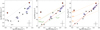 |
Fig. 13 Mass outflow rate vs. nuclear SFR (left panel), outflow momentum rate vs. nuclear SFR (middle panel), and outflow kinetic luminosity vs. nuclear SFR (right panel). Red circles indicate nuclei with outflows launched by an AGN, green diamonds are objects hosting an AGN with molecular outflows of uncertain SF/AGN origin, and stars represent star-formation-dominated nuclei. The blue circles mark the ULIRGs presented in this work. The white stars are the lower luminosity starburts compiled by Cicone et al. (2014). The remaining points correspond to local U/ LIRGs from the literature: NGC 1614 and IRAS 17208–0014 (García-Burillo et al. 2015; Pereira-Santaella et al. 2015; Piqueras López et al. 2016); NGC 3256 N and S (Lira et al. 2002; Pereira-Santaella et al. 2011; Sakamoto et al. 2014; Emonts et al. 2014; Ohyama et al. 2015); ESO 320–G030 (Pereira-Santaella et al. 2016); Arp 220 W (Barcos-Muñoz et al. 2018); and NGC 6240 (Saito et al. 2018). The crosses at the lower right corners represent the typical error bars of the points. The black lines in the left panel correspond to mass loading factors, η = Ṁ /SFR, of 1 and 10. The dashed orange line in the middle panel marks the total momentum injected by SNe as a function of the SFR. The dashed green lines indicate the L(SFR)/c ratio and ten times this value. The dashed orange lines in the right panel indicate the Lout = a × LSNe with a =1, 0.1, and 0.01 as function of the SFR. The solid red lines in the middle and right panels are the best linear fits to the star-formingobjects. |
4.2 Outflow effects on the star formation
The nuclear outflow depletion times are 15−80 Myr, which are comparable to those found in other ULIRGs (Cicone et al. 2014; García-Burillo et al. 2015; González-Alfonso et al. 2017). These times do not include the possible inflow of molecular gas into the nuclear region. However, between 70 and 90% of the molecular gas is already in these central regions (see Tables 3 and 6), so we do not expect significant molecular inflows to occur. Inflows of atomic gas might be present too, but there are no spatially resolved H I observations available for these objects to infer the atomic gas distribution. In addition, we have to take into account that most of the outflowing gas (~60−80%; Table 8) will not escape the gravitational potential of these systems and will become available to form new stars in the future. We can estimate how long it will take for the outflowing gas to rain back into the system from the average outflow velocity, the outflow radius, and the escape velocity (Tables 7 and 8). From the escape velocity we obtain the gravitational parameter, μ = GM, using the relation
 (1)
(1)
where vesc and resc are the escape velocity and the radius at which it is calculated, respectively. Then, assuming that the outflowing gas moves radially and that it is not affected by any dynamical friction, the equations of motion are
 (2)
(2)
with the initial conditions t0 = tdyn, r0 = Rout, and v0 = vout. Integrating these equations numerically, we can determine when r becomes 0, and obtain an estimate of the outflow cycle duration. By doing this, we find cycle durations of 5− 10 Myr (these can be shorter if the dynamical friction is important). Therefore, even if the outflow depletion times are slightly shorter than the SF depletion times (Mtot∕SFR ~ 30−80 Myr), the outflowing gas will return to the starburst region after a few mega-years where it will be available again to form stars. In consequence, the main effects of these outflows are to delay the formation of stars in the nuclear starbursts and to expel a fraction of the total molecular gas (~15−30%) into the intergalactic medium. However, they will not completely quench the nuclear star formation.
Walter et al. (2017) suggested that the molecular outflow detected in the low-luminosity starburst galaxy NGC 253 is accelerating at a rate of 1 km s−1 pc−1 when observed at 30 pc resolution. For these ULIRGs, we find that the higher velocity outflowing molecular gas is not located farther from the nucleus than the lower velocity gas (see Fig. 5 and Appendix B). Therefore, outflow acceleration does not seem to be important for these outflows at the ~500 pc scale and will likely not affect the cycle duration and outflow effects discussed above.
4.3 Outflow launching mechanism in starbursts
There are two main mechanisms that can launch outflows in starbursts. Radiation pressure from young stars can deposit momentum into dust grains. Dust and gas are assumed to be dynamically coupled and, therefore, this process can increase the gas outward velocity and produce an outflow. This class of outflows is known as momentum driven (e.g., Murray et al. 2005; Thompson et al. 2015). The second mechanism is related to the energy injection into the interstellar medium (ISM) by SNe. If the gas does not cool efficiently, this energy increase translates into an adiabatic expansion of the gas, which drives the outflow. These outflows are known as energy driven (e.g., Chevalier & Clegg 1985; Costa et al. 2014).
The scaling relation between the mass loading factor and the outflow velocity is different for energy- and momentum-driven outflows (η ~ v−2 for energy-driven and η ~ v−1 for momentum-driven; e.g., Murray et al. 2005). Cicone et al. (2014) found a slope of –1 for this relation and suggested that the molecular phase of outflows are possibly momentumdriven. However, Fig. 14 shows that, after adding the new data points, the slope of the η vs. v relation is shallower than –1. The best linear fit is
 (3)
(3)
This does not necessarily imply that these outflows are not momentumdriven. Actually, the –1 slope for momentum-driven outflows implicitly ignores the dependency of the outflow velocity on the optical depth, τFIR, of the launching region. When the FIR optical depth increases, the momentum transfer from the radiation to the dust and gas can be considerably more efficient (Hopkins et al. 2013; Thompson et al. 2015). For instance, if τFIR > 1, the momentum boost factor, Ṗout∕(L∕c), can significantly exceed 2 (Thompson et al. 2015).
To test this, in the middle panel of Fig. 13 we plot the outflow momentum rate as a function of the SFR. The best linear fit to the starbursts data is
 (4)
(4)
which has a slope >1. That is, for those starbursts with the lower SFR, the momentum boost factor is approximately 1 (see also Cicone et al. 2014). However, this factor increases for objects with higher SFR up to approximately 8. For one of these starbursts, ESO 320-G030, we measured a very high optical depth in the region launching the outflow ≳8 at 100 μm (Pereira-Santaella et al. 2017). Therefore, higher dust opacities in the more vigorous starbursts could explain these momentum boost factors >2.
We also explore the possible role of SNe in the launching of these outflows. We plot the momentum injected by SNe in the middle panel of Fig. 13, which is more than a factor of ten higher than the radiation pressure. For all the starbursts, the momentum rate of their outflows is lower than the momentum due to SN explosions. Therefore, these outflows could be launched by SNe. If this is the case, the momentum coupling between the SNe and the ISM seems to be more efficient at higher SFR. While for the low SFR objects, the outflows carry less than 10% of the SNe momentum, the outflows in higher SFR objects carry up to 75% of the momentum injected by SNe.
Similarly, in the right panel of Fig. 13, we compare the kinetic luminosity of the outflows with the energy produced by SNe. The outflow kinetic luminosity represents 4− 20% of the energy produced by SNe for the U/LIRGs, whereas for the lower luminosity starbursts, this fraction is ≲1%. Therefore, ifthese outflows are driven by SNe, this suggests that the coupling efficiency between the SNe and the ISM increases with increasing SFR. The best linear fit is
 (5)
(5)
We alsonote that for the AGN U/LIRGs, the observed kinetic luminosities of the outflows are 1− 5% of the AGN luminosity (Cicone et al. 2014; García-Burillo et al. 2015). Thus, if SNe are the main drivers of outflows in starbursts, the coupling between the SN explosions and the ISM must be more efficient than for AGN, at least when the SFR is sufficiently high.
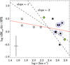 |
Fig. 14 Massloading factor vs. outflow velocity. Only outflows powered by SF are plotted in this figure. Galaxy symbols are as in Fig. 13. The dashed black lines are the best fits with fixed slopes of –1 and –2 (see Sect. 4.3). The red line is the best linear fit. |
4.4 Multi-phase outflows
4.4.1 Outflowing molecular gas evolution
We measure similar outflow dynamical times, around 1 Myr, in all the galaxies. These are much shorter than the age of the star-formation burst expected in ULIRGs (~ 60–100 Myr;Rodríguez Zaurín et al. 2010) and also much shorter than the outflow depletion times (~15–80 Myr; see Sect. 3.4).
This might be connected to the evolution of the gas within the outflow. For instance, if the molecular gas is swept from the nuclear ISM, it might be able to survive only ~1 Myr in the hot gas outflow environment before the molecular gas dissociates and becomes neutral atomic gas (e.g., Decataldo et al. 2017). These dynamical times are also consistent with those measured in the molecular outflow of a local starburst observed at much higher spatial resolution (Pereira-Santaella et al. 2016; Aalto et al. 2016). Alternatively, if the outflow has a bi-conical geometry, its projected area increases proportionally to r2 as it expands. Therefore, even if the molecular gas is not dissociated, its column density rapidly decreases with increasing r and, eventually, the CO emission will be below the detection limit of the observations. The present data do not allow us to distinguish between these possibilities because the outflow structure is just barely spatially resolved and, therefore, it is not possible to accurately measure theradial dependency of the outflow properties. It has been suggested that molecular gas forms in the outflow (e.g., Ferrara & Scannapieco 2016; Richings & Faucher-Giguère 2018). If so, these observations indicate that molecular gas does not efficiently form in outflows, at least beyond 1 kpc or after 1 Myr.
4.4.2 Hot and cold molecular phase
There are observations of the ionized and hot molecular phases of the outflows in I12112, I14348, and I22491 that demonstrate their multi-phase structure and suggest that transitions between the different phases are possible (Arribas et al. 2014; Emonts et al. 2017). For these galaxies, a direct comparison of the CO(2–1) data with the observations of the ionized phase (Hα) are not possible due to the relatively low angular resolution of the Hα data (≳1′′). However, the detection of a broad Hα component indicates the presence of ionized gas in the outflow. The comparison between the cold molecular and the ionized phases of the outflow in NGC 6240 is presented by Saito et al. (2018). They show that the outflow mass is dominated by the cold molecular phase in that object.
For the hot molecular phase, we have maps at higher angular resolution (Emonts et al. 2017). This hot phase is traced by the near-IR ro-vibrational H2 transitions and is detected in three cases (I12112 NE, I14348 SW, and I22491 E). The two cases where no outflow was detected in the hot phase, I12112 SW and I14348 NE, contain the least massive of the CO outflows in our ALMA sample, and may therefore have been below the detection limit of the near-IR data. In general, there is a good agreement between the outflow velocity structures (see Figs. 2–4 of Emonts et al. 2017). Also, there is a good agreement between the average outflow velocities (see Table 10). Interestingly, for the hot molecular H2 gas, only the blueshifted part of the outflows was unambiguously detected. The redshifted part of the outflows, as seen in CO, may have suffered from very high obscuration in the near-IR H2 lines, although the poorer spectral resolution and lower sensitivity of the near-IR data compared to the ALMA data makes this difficult to verify.
The average hot-to-cold molecular gas mass ratio is (2.6 ± 1.0) × 10−5. If we only considered the blueshifted part of the outflows, this ratio would be higher by up to a factor of about 2. These estimates are slightly lower but comparable to the ratio of 6−7 × 10⁻⁵ observed in the outflows of local LIRGs (Emonts et al. 2014; Pereira-Santaella et al. 2016), and well within the 10−7−10−5 range found for molecular gas in starburst galaxies and AGN (Dale et al. 2005). This ratio provides information on the temperature distribution of molecular gas (e.g., Pereira-Santaella et al. 2014) and the excitation of the outflowing gas (e.g., Dasyra et al. 2014; Emonts et al. 2014).
The hot-to-cold molecular gas mass ratio can also be used to obtain a rough estimate of the total outflowing mass of molecular gas when only near-IR H2 data are available. This method was used in Emonts et al. (2017) to extrapolate total molecular mass outflow rates in I12112 NE, I14348 SW, and I22491 E, as based on the near-IR H2 data alone. This resulted in mass outflow estimates that were significantly lower than those found in CO and OH surveys of starburst galaxies and ULIRGs (Sturm et al. 2011; Spoon et al. 2013; Veilleux et al. 2013; Cicone et al. 2014; González-Alfonso et al. 2017). However, our new ALMA results reveal higher molecular mass outflow rates, bringing them back into agreement with these earlier surveys. This shows the importance of directly observing the cold component of molecular outflows, and it highlights the synergy between ALMA and the James Webb Space Telescope for studying the role of molecular outflows in the evolution of galaxies.
Hot molecular outflow phase.
5 Conclusions
We analyzed new ALMA CO(2–1) observations of three low-z ULIRG systems (d ~ 350 Mpc). Thanks to the high S/N and spatial resolution of these data, we were able to study the physical properties and kinematics of the molecular gas around five out of six nuclei of these three ULIRGs. Then, we used data from the literature to investigate the properties of these outflows and their impact on the evolution of the ULIRG systems. The main results of this paper are the following: 1. We have detected fast (deprojected vout ~ 350−550 km s−1; vmax ~ 500−900 km s−1) massive molecular outflows (Mout ~ (0.3−5) × 108 M⊙) in the five well-detected nuclei of these three low-z ULIRGs. The outflow emission is spatially resolved and we measured deprojected outflow effective radii between 250 pc and 1 kpc. The PA of the outflow emission is compatible with an outflow perpendicular to the rotating molecular disk in three cases. Only in one case is the outflow PA clearly not along the kinematic minor axis, suggesting a different outflow orientation. 2. The outflow dynamical times are between 0.5 and 3 Myr and the outflow rates between 12 and 400 M⊙ yr−1. Taking into account the nuclear SFR, the mass loading factors are 0.8 to ~2. These values are similar to those found in other local ULIRGs. The total molecular gas mass in the regions where the outflows originate is (1− 7) × 109 M⊙. Therefore, the outflow depletion times are 15−80 Myr. We also estimate that only 15−30% of the outflowing gas has v > vesc and will escape the gravitational potential of the nucleus. 3. We use multiple indicators to determine the power source of these molecular outflows (e.g., mass loading factor, outflow energy and momentum vs. those injected by SNe, maximum outflow velocity, geometry, etc.). For all the nuclei, the observed molecular outflows are compatible with being powered by the strong nuclear starburst. 4. The outflow depletion times are slightly shorter than the SF depletion times (30−80 Myr). However, we find that most of the outflowing molecular gas does not have enough velocity to escape the gravitational potential of the nucleus. Assuming that the outflowing gas is not affected by any dynamical friction, we estimate that most of this outflowing material will return to the molecular disk after 5− 10 Myr and become available to form new stars. Therefore, the main effects of these outflows are to expel part of the total molecular gas (~ 15−30%) into the intergalactic medium and delay the formation of stars but, possibly, they are not completely quenching the nuclear star formation. 5.Cicone et al. (2014) suggested that outflows in starbursts are driven by the radiation pressure due to young stars (i.e., momentum-driven) based on the –1 slope of the mass loading factor vs. outflow velocity relation. After adding more points to this relation, we find a shallower slope –(0.3 ± 0.2). For momentum-driven outflows, this shallower slope can be explained if the dust optical depth increases for higher luminosity starbursts enhancing the momentum boost factor. One of the nuclear starbursts in our sample has an optical depth ≳8 at 100 μm and might support this scenario. Alternatively, these outflows might be launched by SNe. If so, the coupling efficiency between theISM and SNe increases with increasing SFR. For the stronger starbursts, these molecular outflows carry up to 75 and 20% of the momentum and energy injected by SNe, respectively. 6. We explore the possible evolution of the cold molecular gas in the outflow. The relatively small sizes (<1 kpc) and short dynamical times (<3 Myr) of the outflows suggest that molecular gas cannot survive longer in the outflow environment or that it cannot form efficiently beyond these distances or times. The detection of other outflow phases, hot molecular and ionized, for these galaxies suggests that transformation between the different outflow gas phases might exist. Alternatively, in a uniform bi-conical outflow geometry, the CO column density will eventually be below the detection limit and explain the non-detection of the outflowing molecular gas beyond ~1 kpc. New high-spatial-resolution observations of similar outflows will help to distinguish between these possibilities.
Acknowledgements
We thank the anonymous referee for useful comments and suggestions. M.P.S. acknowledges support from S.T.F.C. through grant ST/N000919/1. L.C., S.G.B., and A.L. acknowledge financial support by the Spanish MEC under grants ESP2015-68964 and AYA2016-76682-C3-2-P. This paper makes use of the following ALMA data: ADS/JAO.ALMA# 2015.1.00263.S, ADS/JAO.ALMA#2016.1.00170.S. ALMA is a partnership of ESO (representing its member states), NSF (USA), and NINS (Japan), together with NRC (Canada), NSC and ASIAA (Taiwan), and KASI (Republic of Korea), in cooperation with the Republic of Chile. The Joint ALMA Observatory is operated by ESO, AUI/NRAO, and NAOJ. The National Radio Astronomy Observatory is a facility of the National Science Foundation operated under cooperative agreement by Associated Universities, Inc.
Appendix A Continuum visibility fits
Figure A.1 compares the real part of the continuum visibilities for each source with the best-fit model discussed in Sect. 3.1.2. To obtain these visibilities, we shifted the phase center to the coordinates obtained by UVMULTIFIT. For the objects with two continuum sources in the field of view, we subtracted the model of the source that is not plotted in that panel.
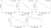 |
Fig. A.1 Real part of the 248 GHz continuum visibilities as function of the uv radius. The red line is the best-fit model discussed in Sect. 3.1.2 (see also Table 4). |
Appendix B CO(2–1)channel maps
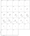 |
Fig. B.1 Channel maps showing the CO(2–1) 230.5 GHz emission in IRAS 12112+0305. Each panel shows the emission averaged over 39 MHz (~50 km s−1) channels. The contours correspond to (3, 6, 12, 24, 48, 96, 192) × σ and σ is the rms measured in each channel (180−260μJy beam−1) for this system. The relativistic LSRK velocity is indicated in each panel. The red crosses mark the location of the nuclei listed in Table 1. |
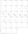 |
Fig. B.2 Same as Fig. B.1 but for IRAS 14348−1447. For this system σ = 200−300μJy beam−1 depending on the channel. |
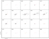 |
Fig. B.3 Same as Fig. B.1 but for IRAS 22491−1808. For this system σ = 250−400μJy beam−1 depending on the channel. |
References
- Aalto, S., Garcia-Burillo, S., Muller, S., et al. 2012, A&A, 537, A44 [NASA ADS] [CrossRef] [EDP Sciences] [Google Scholar]
- Aalto, S., Garcia-Burillo, S., Muller, S., et al. 2015, A&A, 574, A85 [NASA ADS] [CrossRef] [EDP Sciences] [Google Scholar]
- Aalto, S., Costagliola, F., Muller, S., et al. 2016, A&A, 590, A73 [NASA ADS] [CrossRef] [EDP Sciences] [Google Scholar]
- Alonso-Herrero, A., Esquej, P., Roche, P. F., et al. 2016, MNRAS, 455, 563 [NASA ADS] [CrossRef] [Google Scholar]
- Arribas, S., Colina, L., Bellocchi, E., Maiolino, R., & Villar-Martín, M. 2014, A&A, 568, A14 [NASA ADS] [CrossRef] [EDP Sciences] [Google Scholar]
- Barcos-Muñoz, L., Aalto, S., Thompson, T. A., et al. 2018, ApJ, 853, L28 [NASA ADS] [CrossRef] [Google Scholar]
- Bellocchi, E., Arribas, S., Colina, L., & Miralles-Caballero, D. 2013, A&A, 557, A59 [NASA ADS] [CrossRef] [EDP Sciences] [Google Scholar]
- Bolatto, A. D., Wolfire, M., & Leroy, A. K. 2013, ARA&A, 51, 207 [Google Scholar]
- Briggs, D. S. 1995, PhD Thesis, New Mexico Institute of Mining and Technology [Google Scholar]
- Cazzoli, S., Arribas, S., Maiolino, R., & Colina, L. 2016, A&A, 590, A125 [NASA ADS] [CrossRef] [EDP Sciences] [Google Scholar]
- Chevalier, R. A., & Clegg, A. W. 1985, Nature, 317, 44 [NASA ADS] [CrossRef] [Google Scholar]
- Chu, J. K., Sanders, D. B., Larson, K. L., et al. 2017, ApJS, 229, 25 [NASA ADS] [CrossRef] [Google Scholar]
- Chung, A., Yun, M. S., Naraynan, G., Heyer, M., & Erickson, N. R. 2011, ApJ, 732, L15 [NASA ADS] [CrossRef] [Google Scholar]
- Cicone, C., Maiolino, R., Sturm, E., et al. 2014, A&A, 562, A21 [NASA ADS] [CrossRef] [EDP Sciences] [Google Scholar]
- Colina, L., Arribas, S., Borne, K. D., & Monreal, A. 2000, ApJ, 533, L9 [NASA ADS] [CrossRef] [Google Scholar]
- Condon, J. J., Helou, G., Sanders, D. B., & Soifer, B. T. 1990, ApJS, 73, 359 [NASA ADS] [CrossRef] [Google Scholar]
- Condon, J. J., Huang, Z.-P., Yin, Q. F., & Thuan, T. X. 1991, ApJ, 378, 65 [NASA ADS] [CrossRef] [Google Scholar]
- Costa, T., Sijacki, D., & Haehnelt, M. G. 2014, MNRAS, 444, 2355 [NASA ADS] [CrossRef] [Google Scholar]
- Courteau, S. 1997, AJ, 114, 2402 [NASA ADS] [CrossRef] [Google Scholar]
- Dale, D. A., Sheth, K., Helou, G., Regan, M. W., & Hüttemeister, S. 2005, AJ, 129, 2197 [NASA ADS] [CrossRef] [Google Scholar]
- Dasyra, K. M., Combes, F., Novak, G. S., et al. 2014, A&A, 565, A46 [NASA ADS] [CrossRef] [EDP Sciences] [Google Scholar]
- Dasyra, K. M., Bostrom, A. C., Combes, F., & Vlahakis, N. 2015, ApJ, 815, 34 [Google Scholar]
- Dasyra, K. M., Combes, F., Oosterloo, T., et al. 2016, A&A, 595, L7 [NASA ADS] [CrossRef] [EDP Sciences] [Google Scholar]
- Decataldo, D., Ferrara, A., Pallottini, A., Gallerani, S., & Vallini, L. 2017, MNRAS, 471, 4476 [NASA ADS] [CrossRef] [Google Scholar]
- Emonts, B. H. C., Piqueras-López, J., Colina, L., et al. 2014, A&A, 572, A40 [NASA ADS] [CrossRef] [EDP Sciences] [Google Scholar]
- Emonts, B. H. C., Colina, L., Piqueras-López, J., et al. 2017, A&A, 607, A116 [NASA ADS] [CrossRef] [EDP Sciences] [Google Scholar]
- Evans, A. S., Mazzarella, J. M., Surace, J. A., & Sanders, D. B. 2002, ApJ, 580, 749 [NASA ADS] [CrossRef] [Google Scholar]
- Farrah, D., Afonso, J., Efstathiou, A., et al. 2003, MNRAS, 343, 585 [NASA ADS] [CrossRef] [Google Scholar]
- Ferrara, A., & Scannapieco, E. 2016, ApJ, 833, 46 [NASA ADS] [CrossRef] [Google Scholar]
- Feruglio, C., Maiolino, R., Piconcelli, E., et al. 2010, A&A, 518, L155 [NASA ADS] [CrossRef] [EDP Sciences] [Google Scholar]
- Fischer, J., Sturm, E., González-Alfonso, E., et al. 2010, A&A, 518, L41 [NASA ADS] [CrossRef] [EDP Sciences] [Google Scholar]
- García-Burillo, S., Combes, F., Usero, A., et al. 2015, A&A, 580, A35 [NASA ADS] [CrossRef] [EDP Sciences] [Google Scholar]
- García-Marín, M., Colina, L., Arribas, S., Alonso-Herrero, A., & Mediavilla, E. 2006, ApJ, 650, 850 [NASA ADS] [CrossRef] [Google Scholar]
- García-Marín, M., Colina, L., & Arribas, S. 2009a, A&A, 505, 1017 [NASA ADS] [CrossRef] [EDP Sciences] [Google Scholar]
- García-Marín, M., Colina, L., Arribas, S., & Monreal-Ibero, A. 2009b, A&A, 505, 1319 [NASA ADS] [CrossRef] [EDP Sciences] [Google Scholar]
- González-Alfonso, E., Fischer, J., Spoon, H. W. W., et al. 2017, ApJ, 836, 11 [NASA ADS] [CrossRef] [Google Scholar]
- Hill, M. J., & Zakamska, N. L. 2014, MNRAS, 439, 2701 [NASA ADS] [CrossRef] [Google Scholar]
- Hopkins, P. F., Quataert, E., & Murray, N. 2012, MNRAS, 421, 3522 [Google Scholar]
- Hopkins, P. F., Kereš, D., Murray, N., et al. 2013, MNRAS, 433, 78 [NASA ADS] [CrossRef] [Google Scholar]
- Imanishi, M., Nakanishi, K., & Izumi, T. 2016, AJ, 152, 218 [NASA ADS] [CrossRef] [Google Scholar]
- Imanishi, M., Nakanishi, K., & Izumi, T. 2018, ApJ, 856, 143 [NASA ADS] [CrossRef] [Google Scholar]
- Iwasawa, K., Sanders, D. B., Teng, S. H., et al. 2011, A&A, 529, A106 [NASA ADS] [CrossRef] [EDP Sciences] [Google Scholar]
- Kennicutt, R. C., & Evans, N. J. 2012, ARA&A, 50, 531 [NASA ADS] [CrossRef] [Google Scholar]
- Kim, C.-G., & Ostriker, E. C. 2015, ApJ, 802, 99 [NASA ADS] [CrossRef] [Google Scholar]
- Kroupa, P. 2001, MNRAS, 322, 231 [NASA ADS] [CrossRef] [Google Scholar]
- Law, D. R., Steidel, C. C., Erb, D. K., et al. 2009, ApJ, 697, 2057 [NASA ADS] [CrossRef] [Google Scholar]
- Leitherer, C., Schaerer, D., Goldader, J. D., et al. 1999, ApJS, 123, 3 [NASA ADS] [CrossRef] [Google Scholar]
- Lira, P., Ward, M., Zezas, A., Alonso-Herrero, A., & Ueno, S. 2002, MNRAS, 330, 259 [NASA ADS] [CrossRef] [Google Scholar]
- Martí-Vidal, I., Vlemmings, W. H. T., Muller, S., & Casey, S. 2014, A&A, 563, A136 [NASA ADS] [CrossRef] [EDP Sciences] [Google Scholar]
- McMullin, J. P., Waters, B., Schiebel, D., Young, W., & Golap, K. 2007, in Astronomical Data Analysis Software and Systems XVI, eds. R. A. Shaw, F. Hill, & D. J. Bell, ASP Conf. Ser., 376, 127 [NASA ADS] [Google Scholar]
- Murphy, E. J., Condon, J. J., Schinnerer, E., et al. 2011, ApJ, 737, 67 [NASA ADS] [CrossRef] [Google Scholar]
- Murray, N., Quataert, E., & Thompson, T. A. 2005, ApJ, 618, 569 [NASA ADS] [CrossRef] [Google Scholar]
- Narayanan, D., Krumholz, M., Ostriker, E. C., & Hernquist, L. 2011, MNRAS, 418, 664 [NASA ADS] [CrossRef] [Google Scholar]
- Nardini, E., Risaliti, G., Watabe, Y., Salvati, M., & Sani, E. 2010, MNRAS, 405, 2505 [NASA ADS] [Google Scholar]
- Nelson, D., Genel, S., Vogelsberger, M., et al. 2015, MNRAS, 448, 59 [NASA ADS] [CrossRef] [Google Scholar]
- Ohyama, Y., Terashima, Y., & Sakamoto, K. 2015, ApJ, 805, 162 [NASA ADS] [CrossRef] [Google Scholar]
- Papadopoulos,P. P., van der Werf, P., Xilouris, E., Isaak, K. G., & Gao, Y. 2012, ApJ, 751, 10 [NASA ADS] [CrossRef] [Google Scholar]
- Pereira-Santaella, M., Alonso-Herrero, A., Santos-Lleo, M., et al. 2011, A&A, 535, A93 [NASA ADS] [CrossRef] [EDP Sciences] [Google Scholar]
- Pereira-Santaella, M., Spinoglio, L., van der Werf, P. P., & Piqueras López J. 2014, A&A, 566, A49 [NASA ADS] [CrossRef] [EDP Sciences] [Google Scholar]
- Pereira-Santaella, M., Colina, L., Alonso-Herrero, A., et al. 2015, MNRAS, 454, 3679 [NASA ADS] [CrossRef] [Google Scholar]
- Pereira-Santaella, M., Colina, L., García-Burillo, S., et al. 2016, A&A, 594, A81 [NASA ADS] [CrossRef] [EDP Sciences] [Google Scholar]
- Pereira-Santaella, M., González-Alfonso, E., Usero, A., et al. 2017, A&A, 601, L3 [NASA ADS] [CrossRef] [EDP Sciences] [Google Scholar]
- Piqueras López, J., Colina, L., Arribas, S., Alonso-Herrero, A., & Bedregal, A. G. 2012, A&A, 546, A64 [NASA ADS] [CrossRef] [EDP Sciences] [Google Scholar]
- Piqueras López, J., Colina, L., Arribas, S., & Alonso-Herrero, A. 2013, A&A, 553, A85 [NASA ADS] [CrossRef] [EDP Sciences] [Google Scholar]
- Piqueras López, J., Colina, L., Arribas, S., Pereira-Santaella, M., & Alonso-Herrero, A. 2016, A&A, 590, A67 [NASA ADS] [CrossRef] [EDP Sciences] [Google Scholar]
- Pjanka, P., Greene, J. E., Seth, A. C., et al. 2017, ApJ, 844, 165 [NASA ADS] [CrossRef] [Google Scholar]
- Richings, A. J., & Faucher-Giguère, C.-A. 2018, MNRAS, 474, 3673 [Google Scholar]
- Rodríguez Zaurín, J., Tadhunter, C. N., & González Delgado R. M. 2010, MNRAS, 403, 1317 [NASA ADS] [CrossRef] [Google Scholar]
- Rupke, D. S., Veilleux, S., & Sanders, D. B. 2005, ApJ, 632, 751 [Google Scholar]
- Saito, T., Iono, D., Xu, C. K., et al. 2017, ApJ, 835, 174 [NASA ADS] [CrossRef] [Google Scholar]
- Saito, T., Iono, D., Ueda, J., et al. 2018, MNRAS, 475, L52 [NASA ADS] [CrossRef] [Google Scholar]
- Sakamoto, K., Ho, P. T. P., & Peck, A. B. 2006, ApJ, 644, 862 [NASA ADS] [CrossRef] [Google Scholar]
- Sakamoto, K., Aalto, S., Combes, F., Evans, A., & Peck, A. 2014, ApJ, 797, 90 [NASA ADS] [CrossRef] [Google Scholar]
- Salak, D., Nakai, N., Hatakeyama, T., & Miyamoto, Y. 2016, ApJ, 823, 68 [NASA ADS] [CrossRef] [Google Scholar]
- Scannapieco, C., Wadepuhl, M., Parry, O. H., et al. 2012, MNRAS, 423, 1726 [Google Scholar]
- Schaye, J., Crain, R. A., Bower, R. G., et al. 2015, MNRAS, 446, 521 [Google Scholar]
- Spoon, H. W. W., Farrah, D., Lebouteiller, V., et al. 2013, ApJ, 775, 127 [NASA ADS] [CrossRef] [Google Scholar]
- Sturm, E., González-Alfonso, E., Veilleux, S., et al. 2011, ApJ, 733, L16 [NASA ADS] [CrossRef] [Google Scholar]
- Thompson, T. A., Fabian, A. C., Quataert, E., & Murray, N. 2015, MNRAS, 449, 147 [NASA ADS] [CrossRef] [Google Scholar]
- Veilleux, S., Kim, D.-C., & Sanders, D. B. 1999, ApJ, 522, 113 [NASA ADS] [CrossRef] [Google Scholar]
- Veilleux, S., Kim, D., & Sanders, D. B. 2002, ApJS, 143, 315 [NASA ADS] [CrossRef] [Google Scholar]
- Veilleux, S., Rupke, D. S. N., Kim, D.-C., et al. 2009, ApJS, 182, 628 [NASA ADS] [CrossRef] [Google Scholar]
- Veilleux, S., Meléndez, M., Sturm, E., et al. 2013, ApJ, 776, 27 [NASA ADS] [CrossRef] [Google Scholar]
- Veilleux, S., Bolatto, A., Tombesi, F., et al. 2017, ApJ, 843, 18 [Google Scholar]
- Walter, F., Bolatto, A. D., Leroy, A. K., et al. 2017, ApJ, 835, 265 [NASA ADS] [CrossRef] [Google Scholar]
- Westmoquette, M. S., Clements, D. L., Bendo, G. J., & Khan, S. A. 2012, MNRAS, 424, 416 [NASA ADS] [CrossRef] [Google Scholar]
- Wilson, C. D., Petitpas, G. R., Iono, D., et al. 2008, ApJS, 178, 189 [NASA ADS] [CrossRef] [Google Scholar]
See Sect. 10.5.2 of the ALMA Cycle 6 Technical Handbook.
For NGC 3256, we use the newer observations presented by Sakamoto et al. (2014), which distinguish between the northern and southern nuclei, instead of the Sakamoto et al. (2006) data used by Cicone et al. (2014).
All Tables
All Figures
|
Fig. 1 ALMA and HST maps for IRAS 12112+0305. The first and second panels are the CO(2–1) integrated flux and peak intensity for ~10 km s−1 channels, respectively. The contour levels in the second panel correspond to (6, 18, 54, 162, 484) × σ, where σ is the line sensitivity (Table 2). The third panel is the ALMA 248 GHz continuum. The contours in this panel are (3, 27, 81) × σ where σ is the continuum sensitivity (Table 2). The fourth panel shows the near-IR HST/NICMOS F160W map with the CO(2–1) peak contours. The position of the two nuclei is marked with a cross in all the panels. The red hatched ellipse represents the FWHM and PA of the ALMA beam (Table 2). |
| In the text | |
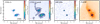 |
Fig. 2 Same as Fig. 1 but for IRAS 14348−1447. |
| In the text | |
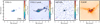 |
Fig. 3 Same as Fig. 1 but for IRAS 22491−1808. |
| In the text | |
|
Fig. 4 For each galaxy of the ULIRG systems, the left- and right-hand panels show the first and second moments of the CO(2–1) emission, respectively. The spacings between the contour levels in the first and second moment maps are 100 and 25 km s−1, respectively.For the first moment maps, the velocities are relative to the systemic velocity (see Table 1). The red box in this panel indicates the field of view presented in Fig. 5 for each object. The dashed and dotted lines mark the kinematic major axis and the outflow axis, respectively, defined in Sect. 3.2 (see also Fig. 5). The black cross marks the position of the 248 GHz continuum peak. The red hatched ellipse shows the beam FWHM and PA. |
| In the text | |
|
Fig. 5 Centroid of the CO(2–1) emission measured in each ~10 km s−1 velocity channel. The color of the points indicates the CO(2–1) velocity with respect to the systemic velocity not corrected for inclination. The rose diamond marks the position of the 248 GHz continuum peak. The dashed line is the linear fit to the low velocity gas and corresponds to the kinematic major axis of the rotating disk. The dotted line is the linear fit to the high-velocity red- and blue-shifted gas, which traces the projection of the outflow axis in the sky. The error bars in each point indicate the statistical uncertainty in the centroid position. The gray error bars represent the astrometric accuracy of these observations for channels with S∕N > 10 (see Sect. 3.2). |
| In the text | |
|
Fig. 6 Rotation curves of the ULIRGs extracted along the kinematic major axis. The red line shows the best fit arctan model to the data. The fit results are presented in Table 5. |
| In the text | |
|
Fig. 7 Blue and red contours in panel a represent the integrated blue- and red-shifted high-velocity CO(2–1) emission, respectively.The specific velocity range is listed in Table 6. The lowest contour corresponds to the 3σ level. The next contour levels are (0.5, 0.9) × the peak of the high-velocity emission when these are above the 3σ level. For I12112 SW, σ = 30 mJy km s−1 beam−1 and the red and blue peaks are at 110 and 240 mJy km s−1 beam−1, respectively. The dotted and the dashed lines are the outflow axis and the kinematic major axis, respectively (see Table 5). The red hatched ellipse represents the beam FWHM and PA. The dashed circle indicates the region from which the nuclear spectrum was extracted. Panel b: nuclear spectrum in yellow and the best-fit model in gray. Panel c: difference between the observed spectrum and the best-fit model. The shaded blue and red velocity ranges in these panels correspond to the velocity ranges used for the contours of panel a. The gray line in panel c marks the 3σ noise level per channel. Panel d: CO(2–1) emission at the velocities indicated by the numbers at the top-right corner of the panel as black and red contours, respectively. The black and red double lines trace the morphological features (spiral arms, tidal tails) observed at those velocities. Panel e: CO(2–1) mean velocity field (same as in Fig. 4). The black dashed line is the kinematic major axis and the gray dot-dashed line is the kinematic minor axis. The far and near sides of the rotating disk are indicated, assuming that the observed morphological features are trailing. |
| In the text | |
|
Fig. 8 Same as Fig. 7 but for I12112 NE. In panel a, σ = 45 mJy km s−1 beam−1 and the red and blue peaks are at 2.4 and 2.9 Jy km s−1 beam−1, respectively. |
| In the text | |
|
Fig. 9 Same as Fig. 7 but for I14348 SW. In panel a, σ = 46 mJy km s−1 beam−1 and the red and blue peaks are at 1.4 and 1.0 Jy km s−1 beam−1, respectively. |
| In the text | |
|
Fig. 10 Same as Fig. 7 but for I14348 NE. In panel a, σ = 32 mJy km s−1 beam−1 and the red and blue peaks are at 0.74 and 0.56 Jy km s−1 beam−1, respectively. |
| In the text | |
|
Fig. 11 Same as Fig. 7 but for I22491 E. In panel a, σ = 43 mJy km s−1 beam−1 and the red and blue peaks are at 1.1 and 2.2 Jy km s−1 beam−1, respectively. |
| In the text | |
|
Fig. 12 Mid- and far-IR spectral energy distribution of the three ULIRGs. The yellow circle corresponds to the Spitzer/MIPS 24 μm flux, the blue squares to the Herschel/PACS 60, 100, and 160 μm fluxes, and the green triangles to the Herschel/SPIRE 250, 350, and 500 μm fluxes. The solid red line is the best fit to the data using a single temperature gray body. |
| In the text | |
|
Fig. 13 Mass outflow rate vs. nuclear SFR (left panel), outflow momentum rate vs. nuclear SFR (middle panel), and outflow kinetic luminosity vs. nuclear SFR (right panel). Red circles indicate nuclei with outflows launched by an AGN, green diamonds are objects hosting an AGN with molecular outflows of uncertain SF/AGN origin, and stars represent star-formation-dominated nuclei. The blue circles mark the ULIRGs presented in this work. The white stars are the lower luminosity starburts compiled by Cicone et al. (2014). The remaining points correspond to local U/ LIRGs from the literature: NGC 1614 and IRAS 17208–0014 (García-Burillo et al. 2015; Pereira-Santaella et al. 2015; Piqueras López et al. 2016); NGC 3256 N and S (Lira et al. 2002; Pereira-Santaella et al. 2011; Sakamoto et al. 2014; Emonts et al. 2014; Ohyama et al. 2015); ESO 320–G030 (Pereira-Santaella et al. 2016); Arp 220 W (Barcos-Muñoz et al. 2018); and NGC 6240 (Saito et al. 2018). The crosses at the lower right corners represent the typical error bars of the points. The black lines in the left panel correspond to mass loading factors, η = Ṁ /SFR, of 1 and 10. The dashed orange line in the middle panel marks the total momentum injected by SNe as a function of the SFR. The dashed green lines indicate the L(SFR)/c ratio and ten times this value. The dashed orange lines in the right panel indicate the Lout = a × LSNe with a =1, 0.1, and 0.01 as function of the SFR. The solid red lines in the middle and right panels are the best linear fits to the star-formingobjects. |
| In the text | |
|
Fig. 14 Massloading factor vs. outflow velocity. Only outflows powered by SF are plotted in this figure. Galaxy symbols are as in Fig. 13. The dashed black lines are the best fits with fixed slopes of –1 and –2 (see Sect. 4.3). The red line is the best linear fit. |
| In the text | |
|
Fig. A.1 Real part of the 248 GHz continuum visibilities as function of the uv radius. The red line is the best-fit model discussed in Sect. 3.1.2 (see also Table 4). |
| In the text | |
|
Fig. B.1 Channel maps showing the CO(2–1) 230.5 GHz emission in IRAS 12112+0305. Each panel shows the emission averaged over 39 MHz (~50 km s−1) channels. The contours correspond to (3, 6, 12, 24, 48, 96, 192) × σ and σ is the rms measured in each channel (180−260μJy beam−1) for this system. The relativistic LSRK velocity is indicated in each panel. The red crosses mark the location of the nuclei listed in Table 1. |
| In the text | |
|
Fig. B.2 Same as Fig. B.1 but for IRAS 14348−1447. For this system σ = 200−300μJy beam−1 depending on the channel. |
| In the text | |
|
Fig. B.3 Same as Fig. B.1 but for IRAS 22491−1808. For this system σ = 250−400μJy beam−1 depending on the channel. |
| In the text | |
Current usage metrics show cumulative count of Article Views (full-text article views including HTML views, PDF and ePub downloads, according to the available data) and Abstracts Views on Vision4Press platform.
Data correspond to usage on the plateform after 2015. The current usage metrics is available 48-96 hours after online publication and is updated daily on week days.
Initial download of the metrics may take a while.