| Issue |
A&A
Volume 616, August 2018
|
|
|---|---|---|
| Article Number | A141 | |
| Number of page(s) | 15 | |
| Section | Cosmology (including clusters of galaxies) | |
| DOI | https://doi.org/10.1051/0004-6361/201833011 | |
| Published online | 04 September 2018 | |
Extended percolation analysis of the cosmic web
1
Tartu Observatory, 61602 Tõravere, Estonia
e-mail: This email address is being protected from spambots. You need JavaScript enabled to view it.
2
ICRANet, Piazza della Repubblica 10, 65122 Pescara, Italy
3
Estonian Academy of Sciences, 10130 Tallinn, Estonia
Received:
13
March
2018
Accepted:
15
May
2018
Abstract
Aims. We develop an extended percolation method to allow the comparison of geometrical properties of the real cosmic web with the simulated dark matter (DM) web for an ensemble of over- and under-density systems.
Methods. We scanned density fields of DM model and Sloan Digital Sky Survey (SDSS) observational samples and found connected over- and under-density regions in a large range of threshold densities. Lengths, filling factors, and numbers of largest clusters and voids as functions of the threshold density were used as percolation functions.
Results. We find that percolation functions of DM models of varying box sizes are very similar to each other. This stability suggests that properties of the cosmic web, as found in the present paper, can be applied to the cosmic web as a whole. Percolation functions depend strongly on the smoothing length. At smoothing length 1 h−1 Mpc the percolation threshold density for clusters is log PC = 0.718 ± 0.014, and for voids such density is log PV = −0.816 ± 0.015; this is very different from percolation thresholds for random samples, which are log P0 = 0.00 ± 0.02.
Conclusions. The extended percolation analysis is a versatile method to study various geometrical properties of the cosmic web in a wide range of parameters. Percolation functions of the SDSS sample are very different from percolation functions of DM model samples. The SDSS sample has only one large percolating void that fills almost the whole volume. The SDSS sample contains numerous small isolated clusters at low threshold densities, instead of one single percolating DM cluster. These differences are due to the tenuous DM web, which is present in model samples but absent in real observational samples.
Key words: large-scale structure of Universe / dark matter / cosmology: theory / galaxies: halos / methods: numerical
© ESO 2018
1. Introduction
Studies of the three-dimensional distribution of galaxies show that galaxies and clusters of galaxies are not randomly clustered. Chains and filaments connect galaxies and clusters to a continuous supercluster-void network (Jõeveer & Einasto 1977, 1978 Jõeveer et al. 1978; Gregory & Thompson 1978; Einasto et al. 1980; Zeldovich et al. 1982), which is presently called the cosmic web (Bond et al. 1996). The cosmic web is a complex system and the number of methods to describe the web in quantitative terms is rapidly growing. Recent reviews of methods to characterise the structure of the web were given among others by van de Weygaert & Schaap (2009), Aragon-Calvo et al. (2010b), and Libeskind et al. (2018). An overview of the present status of the study of the cosmic web can be found in the Zeldovich symposium proceedings (van de Weygaert et al. 2016).
One essential geometrical property of the cosmic web is the connectivity of components of the web. Clusters are connected by filaments to superclusters and to the whole web, and similarly voids form a complex system connected by tunnels. The connectivity property is analysed in percolation theory and is applied in physics, geophysics, medicine etc.; for an introduction to percolation analysis, see Stauffer (1979). The percolation method was introduced in cosmological studies by Zeldovich et al. (1982), Melott et al. (1983), and Einasto et al. (1984). Its principal idea was explained by Shandarin (1983). In these first studies the percolation method was applied to particles and galaxies.
A natural extension of the method is to use the density field instead of particles, this permits the study of the connectivity of over- and under-dense regions. Using an appropriate threshold density the field is divided into high-density and low-density regions. Connected high-density regions are called clusters and connected low-density regions are called voids. If the threshold is high, then clusters are small and are isolated from each other. When the threshold density decreases then clusters start to merge, and at certain threshold density the largest cluster spans the whole volume under study. This threshold is called percolating density threshold. Similarly the connectivity of voids can be investigated. The percolation method using density fields was applied by Einasto et al. (1986, 2014), Einasto & Saar (1987), Boerner & Mo (1989), Mo & Boerner (1990), Dominik & Shandarin (1992), Klypin & Shandarin (1993), Yess & Shandarin (1996), Yess et al. (1997), Sahni et al. (1997), Sathyaprakash et al. 1998a,b), and Shandarin et al. (2004, 2006). Percolation processes were also used to identify elements of the cosmic web. Aragon-Calvo et al. (2007) applied the Multiscale Morphology Filter to identify clusters, filaments, and walls of the cosmic web. Cautun et al. (2013, 2014) developed the NEXUS and NEXUS+ algorithms to identify filaments and sheets by finding the threshold at which filament and sheet networks percolate.
So far the percolation analysis has been concentrated to the study of properties of clusters and voids near to the percolating threshold density. Most percolation studies were only applied to the study of connectivity of simulated dark matter (DM) samples. The goal of this paper is to develop and test a modification of the percolation method. The extended version of the percolation analysis differs from most previous percolation analyses as follows: (i) we use a wide threshold density interval to find cluster and void lengths and filling factors; (ii) we use a large range of smoothing lengths to describe the density field of DM and galaxies in a complex way; and (iii) we apply percolation analysis to compare DM models with observations. We use only positional data that are available for DM particles and galaxies, and ignore velocities that are available only for particles. We consider DM as a physical fluid having continuous density distribution, thus simulated DM particles are only markers of the field. Similarly we consider observed galaxies as markers of a smooth luminosity density field.
We divide the cosmic web under study at each threshold density into high- and low-density systems, clusters, and voids. For each threshold density we find catalogues of clusters and voids, and select the largest clusters and largest voids. Lengths and volumes of largest clusters and voids, and numbers of clusters and voids at respective threshold density levels, as functions of the threshold density, are used as percolation functions. Percolation functions allow an easy, very compact, and intuitive presentation of general geometrical properties once for the whole web, i.e. ensembles of all clusters and voids for a particular parameter set. Catalogues of clusters and voids are essential parts of the method and provide information on individual clusters and voids.
We use the density field estimator with a constant grid, as applied in numerical simulations of the evolution of the cosmic web. The density field found in numerical simulations presents the true density of the DM model. To compare models with observations it is important to apply a proper smoothing level suited for a particular task. We use smoothing kernel sizes from 1 to 8 h−1 Mpc to see the effect of smoothing to geometrical properties of the web.
To see the dependence of percolation properties on the size of the sample, we use numerical simulations of the evolution of the web, applying cold dark matter (CDM) cosmology in boxes of sizes from 100 to 1024 h−1 Mpc. In all models we use cosmological parameters: Hubble parameter H0 = 100 h km s−1 Mpc−1, matter density parameter Ωm = 0.28, and dark energy density parameter ΩΛ = 0.72. Density fields of simulated CDM samples are given for grid sizes from ~0.2 to 2 h−1 Mpc. This is sufficient to investigate global geometrical properties of our observed and simulated samples. For comparison we use the main sample of the Sloan Digital Sky Survey (SDSS) data release 8 (DR8) survey to calculate the luminosity density field of galaxies.
The paper is organised as follows. In the next section we describe the calculation of the density field of observed and simulated samples along with the method to find clusters, voids, and their parameters. In Sect. 3 we perform percolation analysis of DM simulated clusters and voids. In Sect. 4 we compare percolation properties of the model and SDSS samples. The last section provides a general discussion and summary remarks.
2. Data and methods
2.1. Simulations of the evolution of the cosmic web
Simulations of the evolution of the cosmic web were performed in boxes of sizes L0 = 100, 256, 512, 1024 h−1 Mpc with resolution Ngrid = 512 and  particles. This wide interval of simulation boxes was used to investigate the influence of the simulation box on percolating properties of models. We designated the simulations as L100, L256, L512, and L1024. The initial density fluctuation spectra were generated via the COSMICS code by Bertschinger (1995). We assumed cosmological parameters Ωm = 0.28, ΩΛ = 0.72, σ8 = 0.84 and the dimensionless Hubble constant h = 0.73. To generate initial data we used the baryonic matter density Ωb = 0.044 (Tegmark et al. 2004). Calculations were performed with the GADGET-2 code by Springel (2005). Particle positions were extracted for seven epochs between redshifts z = 30 − 0. The cell size of the simulation L512 is L0/Ngrid = 1 h−1 Mpc, which is identical to the size of cells of the density field of observational SDSS main sample of galaxies used by Liivamägi et al. (2012).
2.2. SDSS data
The density field method facilitates using flux-limited galaxy samples and taking statistically into account galaxies too faint to be included in the flux-limited samples, as applied among others by Einasto et al. (2003, 2007) and Liivamägi et al. (2012) to select superclusters of galaxies.
We used the SDSS DR8 (Aihara et al. 2011) and galaxy group catalogue by Tempel et al. (2012) to calculate the luminosity density field. In the calculation of the luminosity density field we needed to take into account the selection effects that are present in flux-limited samples (Tempel et al. 2009; Tago et al. 2010). In the calculation of the luminosity density field, galaxies were selected within the apparent r magnitude interval 12.5 ≤ mr ≤ 17.77 (Liivamägi et al. 2012). In the nearby region relatively faint galaxies are included to the sample; in more distant regions only the brightest galaxies are seen. To take this into account, we calculated a distance-dependent weight factor (1)
(1)
where L1,2 = L⊙100.4(M⊙−M1,2) are the luminosity limits of the observational window at distance d, corresponding to the absolute magnitude limits of the window M1 and M2. The weight factor WL(d) increases to ≈8 at the far end of the sample; for a more detailed description of the calculation of the luminosity density field and corrections used, see Liivamägi et al. (2012).
2.3. Calculation of the density field
In numerical simulations of the evolution of the cosmic web for each simulation step the density field with resolution L0/Ngrid h−1 Mpc was calculated to find the gravitational potential field and vice versa. We extracted particle positions and density fields at each simulation epoch, which represent true densities of our DM models.
We determined smoothed density fields of galaxies and simulations using a B3 spline (see Martínez & Saar 2002), (2)
(2)
The spline function is different from zero only in the interval x ∈ [−2, 2]. To calculate the high-resolution density field we used the kernel of the scale, which is equal to the cell size of the simulation, L0/Ngrid, where L0 is the size of the simulation box and Ngrid is the number of grid elements in one coordinate. The smoothing with index i has a smoothing radius ri = L0/Ngrid × 2i. The effective scale of smoothing is equal to 2 × ri.
To investigate the influence of the smoothing length, we calculated density fields with smoothing up to index 5. For the L100 model smoothing with indexes, i = 2, 3, 4, 5 corresponds to kernels of radii 0.78, 1.56, 3.125, 6.25 h−1 Mpc; for the L256 model indexes, i = 1, 2, 3, 4 correspond to kernels of radii RB = 1, 2, 4, 8 h−1 Mpc; for the L512 model smoothing indexes, i = 1, 2, 3 correspond to kernels of radii RB = 2, 4, 8 h−1 Mpc; and for the L1024 model indexes, i = 1, 2 correspond to kernels of radii 4, 8 h−1 Mpc. The comparison between the B3 spline kernel and Gaussian kernel is given in Appendix C of Tempel et al. (2014c). The B3 kernel of radius RB = 1 h−1 Mpc corresponds to a Gaussian kernel with dispersion RG = 0.6 h−1 Mpc.
2.4. Finding clusters and voids
The main step in the percolation method is finding the overdensity and under-density regions of the density field. We call over-density regions geometrical clusters and under-density regions geometrical voids, or briefly clusters and voids. The difference between geometrical clusters and voids, and physical clusters and voids is discussed below. In the cluster search we used several loops over the density field. The first loop is over threshold densities.
We scan the density field in a range of threshold densities from Dt = 0.1 to Dt = 10 in mean density units. For our study the behaviour of voids is critical, thus we use a logarithmic step of densities, log Dt = 0.02, to find over- and under-density systems. In this way there are the same number of steps in regions below and above the mean density level. This range covers all densities of practical interest, since in low-density regions the minimal density is ≈0.1 and the density threshold to find conventional superclusters is Dt ≈ 5 (Liivamägi et al. 2012). We mark all cells with density values equal or above the threshold Dt as filled regions and all cells below this threshold as empty regions.
Inside the first loop we make another loop over all filled cells to find neighbours among filled cells. Two cells of the same type are considered as neighbours (friends) and members of the cluster if they have a common sidewall. Every cell can have at most six cells as neighbours; in percolation theory this is called site percolation (Klypin & Shandarin 1993). Members of clusters are selected using a Friend-of-Friend (FoF) algorithm: the friend of my friend is my friend.
When a cluster is found, the next step is the calculation of its parameters. We calculate the following parameters: centre coordinates, xc, yc, zc (mean values of extreme x, y, z coordinates); sizes along coordinate axes, Δx, Δy, Δz (differences between extreme x, y, z coordinates); geometrical diameters,  ; maximal sizes along coordinate axes, Lmax = max(Δx, Δy, Δz); volumes, VC, defined as the volume in space in which the density is equal or greater than the threshold density Dt; and total masses (or luminosities), Mt, i.e. the masses (luminosities) inside the density contour Dt of the cluster, both in mean density units.
During the cluster search we find the cluster with the largest volume for the given threshold density. We store in a separate file for each threshold density the number of clusters found, and data on the largest cluster: the geometrical diameter, maximal size along coordinate axes, volume, and total mass (luminosity). Diameters and maximal sizes are expressed in units of the sample size, L0 (the effective side length in the case of the SDSS sample), the volume (actually the filling factor) is expressed in units of the volume of the whole sample, V0. Maximal sizes (lengths) of largest clusters, ℒ(Dt) = Lmax/L0, filling factors of largest clusters, ℱ (Dt) = Vmax/V0, and numbers of clusters at the threshold density, N(Dt), as functions of the threshold density, Dt, are percolation functions that characterise general geometrical properties of the web. If the cluster spans the whole volume under study, Lmax = L0, the cluster is called percolating. The percolation threshold density, P = Dt, is defined as follows: for Dt ≤ P there exists one and only one percolating cluster, for Dt > P there are no percolating clusters (Stauffer 1979).
A similar procedure is used to find voids. A loop over all empty cells is made to find neighbours among other empty cells. The search for neighbours is made exactly the same way as the search of over-density regions. Parameters of voids are found using the same procedure. This procedure uses as input only the catalogue of marked cells, i.e. either over-density or underdensity cells. As in the case of clusters we find for each threshold density the largest voids, and store in a separate file the number of voids at this threshold and the parameters of largest voids. The lengths and filling factors of largest voids and the numbers of voids as functions of the threshold density are percolation functions of voids. The percolation threshold P of voids is defined inversely: for Dt ≥ P there exists one percolating void, for Dt < P there are no percolating voids.
During the search of high- and low-density systems we exclude very small systems to avoid the contamination of cluster and void catalogues with very small systems. For most samples we carry out two cluster and void searches, using exclusion volume limits, N lim = 50 and 500 computation cells. For the geometry study we use mostly the largest system in each cluster and void catalogue; the length function ℒ(Dt) and the filling factor function ℱ (Dt) are not influenced by the choice of Nlim. Clusters and voids found for close threshold densities usually have rather similar properties. But close to the percolation threshold density clusters (voids), found for neighbouring Dt values, have rather different lengths and volumes; in this Dt range percolation functions change rapidly with Dt.
Our scanning procedure of density fields is constructed in a way that every grid cell is classified as being part of a cluster or void. Most cells are classified as members of clusters at one threshold density value and as members of voids at another threshold density value. The procedure is different from conventional methods in which a cell can be part of only one type of structure element (node, wall, filament, or void; Cautun et al. 2014). In total we have 101 steps and find for each smoothing length 101 catalogues of clusters and 101 catalogues of voids. As we have four models with different size, four smoothing lengths, and clusters and voids separately, we have 16 percolation function pairs, and 4 × 4 × 2 × 101 = 3232 cluster and void catalogues. Catalogues of clusters and voids for each search parameter contain large quantities of information. These catalogues were also stored, and selectively used in the present paper.
3. Extended percolation analysis of DM model samples
In this section we apply the extended percolation method to analyse properties of DM model samples. We focus on how percolation properties evolve with time, how smoothing length influences geometrical properties of the density field, and what are the principal similarities and differences of properties of the ensemble of clusters from properties of the ensemble of voids.
3.1. Geometrical versus physical clusters and voids
As is traditional in percolation analyses, we call high-density regions clusters and low-density regions voids. The terms clusters and voids in our context are geometrical clusters and geometrical voids. Geometrical clusters can have as subclusters physical clusters or superclusters that are connected by filaments and sheets. Similarly geometrical voids may consist of physical voids that are connected by intermediate-density tunnels. Physical clusters may be defined as compact galaxy systems (Huchra & Geller 1982; Tago et al. 2010; Tempel et al. 2014c) and physical voids as low-density regions that are surrounded by galaxies (Einasto et al. 1989; Colberg et al. 2008). Alternatively physical clusters and superclusters can be defined by velocity inflow (Tully et al. 2014), and physical voids can be defined by single-stream regions that have not undergone shell-crossing (Falck & Neyrinck 2015) or by velocity outflow (Sorce et al. 2016). An universal physical void identification tool VIDE was suggested by Sutter et al. (2015). For the difference between geometrical and physical clusters and voids see also Dominik & Shandarin (1992) and Sheth et al. (2003).
3.2. Percolation functions at various stages of the evolution of the cosmic web
To understand geometrical properties of the cosmic web at various stages of its evolution we calculated percolation functions for five epochs of the evolution of the cosmic web, corresponding to redshifts z = 30, 10, 3, 1, and the present epoch, z = 0. Functions were calculated for the model L512, using original density fields without additional smoothing, as found from simulations. During the search of over- and under-density regions the limit to exclude very small systems was in these calculations set to Nlim = 500 computation cells, i.e. cubic h−1 Mpc. For this reason total numbers of clusters and voids are smaller than in most other calculations, as seen in Table 1. Properties of largest clusters and voids are not influenced by this difference.
Table 1 and Fig. 1 show how percolation functions change during the evolution of the cosmic web and obtain the form at the present epoch. At the early epoch z = 30 there are no voids at threshold densities Dt ≤ 0.8, and no clusters at Dt ≥ 1.2. As the evolution proceeds, the interval of threshold densities, where clusters and voids exist, increases. At early epochs percolation functions of clusters and voids are rather symmetrical in logarithmic scale. This symmetry is gradually lost during the evolution.
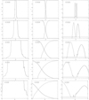 |
Fig. 1. Change of percolation functions of the model L512 with simulation epoch. Panels from top to bottom are for the initial epoch, z = 30, and epochs z = 10, z = 3, z = 1, and z = 0. Left panels: lengths of largest clusters and voids, ℒ(Dt) = Lmax/L0; centre panels: filling factors of largest clusters and voids, ℱ (Dt) = Vmax/V0; right panels: numbers of clusters and voids, N(Dt); all as functions of the threshold density, Dt. Functions are found for original non-smoothed density fields, which correspond to a resolution 1 h−1 Mpc. Functions for clusters are plotted with solid lines, for voids with dashed lines. |
One measure of the connectivity of the web is the percolation threshold density, which is found for both clusters and voids, PC and PV. Table 1 and Fig. 1 show the change of the percolation threshold density of clusters and voids with the evolution epoch, z. At the early epoch z = 30 the distribution of densities is almost Gaussian and symmetric around the mean density, Dt = 1.0. Percolation functions at early epochs are very close to respective functions for purely random samples (Einasto et al. 1986). Thus the change of percolation threshold density with epoch describes the growth of departures from the initial Gaussian density field to its present non-Gaussian form.
The spread of densities around the mean density D = 1.0 is at early epochs proportional to the amplitude of density perturbations. At the recombination epoch, z ≈ 1000, the amplitude of density perturbations is of the same order, δ = D − 1.0 ≈ 10−3. The departure of percolation density threshold for clusters from the mean density value, D = 1.0, is of the same order, PC ≈ 1 + 10−3. Similarly, the departure of percolation density threshold for voids from unity is PV ≈ 1 − 10−3. Both for clusters and voids the limiting values of percolation density thresholds of random Gaussian samples are very close to 1.0. We accept as the percolation density threshold for random samples the geometric mean of percolation threshold density for z = 30 and z ≈ 1000: PC0 = 1.06 ± 0.03 for clusters, and PV0 = 0.94 ± 0.03 for voids, or approximately P0 = 1.00 ± 0.05 for both. The departure of percolating threshold densities from these values can be used as a measure of the departure of the density field from a Gaussian field.
Percolation parameters of model and SDSS clusters and voids.
3.3. Percolation functions of DM clusters and voids
We consider first the percolation functions of DM model clusters, i.e. high-density regions above the threshold density D t in our simulations, which are plotted on Fig. 2. At very high threshold density there exists only a few high-density regions – peaks of density field as ordinary clusters of galaxies. These peaks are isolated from each other and they cover a small filling factor in space. When we lower the threshold density, the number of clusters increases, as well as the filling factor of the largest cluster. At certain threshold density, Dt ≈ 5, depending on the smoothing scale and the size of the computational box, the number of clusters reaches a maximum. At this threshold density large clusters still covers a low filling factor and have lengths of less than the size of the sample. Most large clusters have the form of conventional superclusters, consisting of high-density knots joined by filaments to a single system.
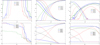 |
Fig. 2. Percolation functions of model and observational samples: left panels: lengths of largest clusters and voids, ℒ(Dt) = Lmax/L0; centre panels: filling factors of largest clusters and voids, ℱ (Dt) = Vmax/V0; right panels: numbers of clusters and voids, N(Dt), as functions of the threshold density, Dt. Lengths and filling factors are expressed in units of the total lengths and volumes of samples. Top panels represent the DM model L512; bottom panels represent the SDSS samples. Percolation functions are found using smoothing kernels of radii 1, 2, 4, and 8 h−1 Mpc. Solid lines show data on clusters, and dashed lines on voids. Indices show the smoothing kernel length in h−1 Mpc. Number functions N(Dt) of DM models in this figure correspond to small system excursion limit Nlim = 50 cells. |
When the threshold density still decreases, the length of the largest cluster increases very rapidly, supercluster-like systems merge, and at threshold Dt = PC the largest cluster reaches opposite sidewalls of the model. Since our models are periodic boxes, this means that the cluster is actually infinite in length. The percolation threshold depends on the box size and smoothing length. We investigate this dependence in more detail below. Data for just percolating clusters and voids are given in Table 1: percolating threshold densities PC and PV, numbers of clusters and voids, NC and NV, and filling factors at percolating threshold densities, FC and FV.
Now consider percolation functions of voids. At a very small threshold density, Dt ≪ 0.1, there are no voids at all. Voids appear at a certain threshold density level, depending on the smoothing kernel, and their number rapidly increases with increasing Dt. At a very low threshold density void sizes are small; they form isolated bubbles inside the large over-density cluster and the filling factor of the largest void is very small. Voids in the density field have at the smallest threshold density the length of the largest void, ℒV(Dt) ≤ 0.5, depending on the smoothing scale and size of the model. Void bubbles are separated from each other by DM sheets. Some sheets have tunnels that permit the formation of some larger connected voids. With increasing threshold density the role of tunnels rapidly increases and tunnels join neighbouring voids. At certain threshold density (Dt ≈ 0.2 for small smoothing lengths) the largest void is percolating, but still not filling a large portion of the volume. When we use larger smoothing lengths then expanded highdensity regions block tunnels between voids at small threshold density and percolation occurs at higher Dt.
The number of voids has a maximum at threshold density Dt ≈ 0.1 for the density field of smoothing scale 1 h−1 Mpc. With increasing smoothing scale the maximum shifts to larger Dt. For Dt ≥ 1 there is only one large percolating void; its filling factor increases with the increase of Dt.
3.4. Influence of smoothing scale to describe cosmic web
According to the presently accepted CDM paradigm, density fluctuations of all scales exist. This leads to fractal nature of the distribution of DM and galaxies with a transition to homogeneity on large scales (Mandelbrot 1982; Jones et al. 1988; Einasto & Gramann 1993). The hierarchical character of DM distribution is well seen in voids with sub-voids and sub-sub-voids, etc. (Aragon-Calvo et al. 2010a,b; Aragon-Calvo & Szalay 2013). The fractal structure has no preferred scales. However, physical processes on different scales are different. On small scales inside haloes non-gravitational (hydrodynamical) processes are dominant. The study of haloes is a separate topic in which particular questions are asked regarding, for example galaxy formation (White & Rees 1978), galaxy evolution (Tinsley 1968), and the number of galactic satellites (Klypin et al. 1999). On larger scales purely gravitational processes are dominant. We can ask at which scale the transition from non-gravitational to gravitational character of processes occurs.
Within haloes dark and baryonic matters are separated. Luminous matter forms visible populations of main galaxies and satellite galaxies. A fraction of baryonic matter within haloes is in the form of diffuse hot coronas of main galaxies. Using catalogues of luminous galaxies and applying appropriate smoothing it is possible to restore approximately the distribution of baryonic matter for comparison with smooth distribution of DM.
Radii of DM haloes can be estimated using visible objects, such as satellites around giant galaxies. Early estimates have already shown that radii of DM haloes around galaxies are of the order of 1 h−1 Mpc (Einasto et al. 1974), which has been confirmed by recent observations of velocities of galaxies in the nearby volume of space: satellites of giant galaxies have orbital velocities up to a distance ≈1 h−1 Mpc from the central galaxy. At a larger distance the smooth Hubble flow dominates (Karachentsev et al. 2002), showing the transition from DM dominated haloes to filaments. This limit corresponds to a smoothing kernel radius ≈ 0.6 h−1 Mpc.
Tempel et al. (2014b) searched for filaments in SDSS main galaxy survey and found that characteristic radii of galaxy filaments are 0.5 h−1 Mpc. These authors showed that filaments of such radius have the strongest impact on galaxy evolution parameters. Actually the radius of filaments can be a bit larger, of the same order as the size of DM haloes of bright galaxies.
We chose 1 h−1 Mpc as the scale of transition from dominantly non-gravitational to gravitational character of processes. We consider the structure on smaller scales as the topic of galactic haloes, the structure on larger scales the topic of the cosmic web, and smoothing with kernel length RB = 1 h−1 Mpc as representing the true density field of gravitating matter of the web. We use smoothing with larger kernels for methodical purposes to understand properties of the web on various scales, following among others Aragon-Calvo et al. (2007), Cautun et al. (2013 and 2014). Percolation functions, calculated for density fields with smoothing scales 1 and 2 h−1 Mpc, are plotted in Fig. 2 by bold lines; the scale 2 h−1 Mpc is available in all our DM models. The B3 kernels RB = 1, 2 h−1 Mpc correspond to Gaussian kernels RG = 0.6, 1.2 h−1 Mpc.
The contrast in the behaviour of clusters and voids is largest when we use original density fields of models. Smoothing shifts part of DM from high-density regions to their surrounding, increases filling factors of clusters and decreases filling factors of voids, especially on small and medium threshold densities. In this way smoothing decreases density contrast, which leads to the decrease of percolation thresholds of clusters and to the increase of percolation thresholds of voids.
3.5. Comparison of models of different size
Table 1 shows clearly that percolation functions of DM models of varying size are very similar to each other for identical smoothing lengths. We use this similarity to define percolation parameters of samples. One of the principal geometrical properties of the cosmic web is the connectivity of overand under-density regions, or clusters and voids in our terminology. The connectivity can be measured by the percolation threshold density of clusters and voids.
In Fig. 3 we show percolation threshold densities as functions of the smoothing kernel length, RB. Data are given for all our models and smoothing lengths. The figure shows that there is a very close relationship of percolation threshold densities and the smoothing kernel length, both for clusters and voids. The relationship between PC and RB is very close and almost linear in log-log representation, (3)
(3)
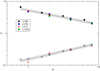 |
Fig. 3. Percolation threshold of clusters and voids, PC and PV, of models L100, L256, L512, L1024 for various smoothing lengths RB. Filled symbols are for clusters, open symbols for voids. Linear fits according to Eq. (3) are shown by solid lines, 95% confidence limits by dashed lines. |
and there is a similar equation for void percolation threshold densities, PV and RB. Constants of equations have values aC = 0.718 ± 0.014, bC = −0.444 ± 0.025 for clusters and aV = −0.816 ± 0.015, bV = 0.503 ± 0.027 for voids. The scatter of individual values from the mean relationship is rather small. At RB = 1 the percolation threshold of clusters is log PC(1) = 0.718 ± 0.014, or PC(1) = 5.23 ± 0.31, and of voids is log PV(1) = −0.816 ± 0.015, or PV(1) = 0.152 ± 0.012. The deviation from the percolation threshold density from a random distribution with log P0 = 0.00 ± 0.05 (or more exactly PC0 = 1.06 ± 0.03 and PV0 = 0.94 ± 0.03) is very clear, and exceeds the mean scatter of values around the mean relationship by a large margin.
The relationship between PC and RB (and between PV and RB) is the same for all models, in spite of large differences of sizes of models from L = 100 to L = 1024 h−1 Mpc. Actually the relationship (3) is valid even on a broader scale. Einasto et al. (1986) found log PC = 0.55 and log PV = −0.70, for a CDM model of box length 40 h−1 Mpc, using smoothing scale ≈1.25 h−1 Mpc, which is not far from our present results. This means that the percolation threshold density is a well-defined and stable characteristic of DM model samples.
Filling factors of largest clusters and voids at mean threshold density, Dt = 1.0, depend on the smoothing kernel size, as seen in Fig. 4. We can express this relationship as follows: (4)
(4)
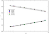 |
Fig. 4. Filling factors of largest clusters and voids at mean threshold density, ℱC(1) and ℱV(1), of models L100, L256, L512, L1024 for various smoothing lengths RB. Filled symbols indicate clusters; open symbols indicate voids. Linear fits according to Eq. (4) are shown by solid lines, 95% confidence limits by dashed lines. |
and there is a similar equation for voids. We get for constants of the equation values: fC = 0.1652 ± 0.0028, gC = 0.1992 ± 0.0051; and for voids fV = 0.8286 ± 0.0028, gV = −0.1962 ± 0.0050. From these constants we get ℱC(1)+ℱV(1) = 0.9938; the summed filling factors of largest clusters and voids at smoothing length RB = 1.0. It is a bit less than unity, since small isolated clusters and voids, other than the largest of these, have very small volumes. We see that filling factors of the largest clusters and voids at mean threshold densities of all our models fit the same relationship very accurately.
If the relationship (4) is valid for larger smoothing kernels, then at RB ≈ 30 h−1 Mpc filling factors of clusters and voids at mean threshold densities become equal, and at still larger kernels cluster filling factors exceed filling factors of voids. The kernel RB ≈ 30 h−1 Mpc corresponds to Gaussian kernel RG ≈ 18 h−1 Mpc.
3.6. Total filling factors
So far we have used only filling factors of largest clusters and voids to characterise properties of the web. Now we also discuss the relationship between total filling factors and the filling factors of the largest systems. We show in Fig. 5 total filling factors of high- and low-density regions, ℱtot, and the filling factors for maximal clusters and voids, ℱmax, as functions of threshold density, Dt. The top panel shows filling factor functions for the L512 model; functions for other models are very similar. The bottom panel shows similar functions for SDSS samples. The left and right panels show filling factor functions applying smoothing kernel radii RB = 2, 8 h−1 Mpc, respectively.
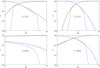 |
Fig. 5. Filling factor functions of the model L512: total filling factors of clusters and voids, ℱtot, and filling factors of maximal clusters and voids, ℱmax, as functions of threshold density, Dt, plotted in logarithmic scales. Solid lines indicate total filling factors of high- and low-density regions, dashed lines indicate maximal clusters and voids, blue indicates clusters, and black indicates voids. Functions are calculated using smoothing kernels 2 and 8 h−1 Mpc (left and right panels). Bottom row: the same functions for observed SDSS samples. |
Filling factor functions for models of various box sizes but identical smoothing kernels are rather similar, both for clusters and voids. As expected, the size of the smoothing kernel has a large effect to filling factor functions. At threshold density Dt = 10 models of all sizes and smoothing kernel RB = 2 h−1 Mpc have total filling factor of clusters ℱtot ≈ 10−2. At threshold level Dt = 0.1 and the same smoothing kernel the total filling factors of voids are ℱtot ≈ 0.03; this is the case for models of all sizes. Larger smoothing with kernel RB = 8 h−1 Mpc decreases the threshold density of clusters at the same total filling factor to Dt ≈ 3 and increases the threshold density of voids to Dt ≈ 0.2.
At small threshold density, Dt ≤ 1, DM samples have ℱmax ≈ ℱtot, i.e. the largest cluster fills the whole over-density volume. In other words, the summed volume of all clusters except the largest cluster is small or zero. When we compare these functions at higher threshold densities, we see that the filling factor of the largest cluster decreases rapidly with increasing Dt, and total filling factors of smaller clusters increases, i.e. curves for ℱtot and ℱmax diverge.
The behaviour of filling factor functions for voids is opposite. For large threshold densities the filling factors of the largest void are equal to the total filling factors; only one large void exists. At lower threshold densities the fraction of small voids increases and functions for ℱtot and ℱmax diverge.
The Table 1 shows that filling factors of largest clusters and voids at percolation levels, ℱC(Dt = P), as functions of the smoothing scales of models, RB, have a larger scatter than the relationship (4). This means that there are small differences between models of different sizes. For small smoothing lengths (RB = 1, 2) filling factors of largest DM clusters at percolating threshold is ℱC(P) ≈ 10−2, and of largest DM voids ℱV(P) ≈ 5 × 10⁻², for models of all sizes.
Sahni et al. (1997) calculated percolation functions in the form νmax = Fmax/Ftot, and plotted these as functions of Ftot, and of density contrast, δt = 1 − Dt, both for clusters and for voids. These representations are complementary to the representations presented in Figs. 2 and 5.
3.7. Topological properties of the cosmic web
Percolation functions are not meant to describe topological properties of the cosmic web in such a way as the genus and Minkowski functional approaches allow. However, our data are sufficient to make a distinction between the main types of topology: cellular or Swiss-cheese type, sponge-like, and meatball-like. The distinction between these topologies is given by the percolating threshold densities of clusters and voids. Cellular topology corresponds to the case when clusters are percolating, but voids are not percolating. If both clusters and voids are percolating then we have the sponge topology. When voids are percolating, but clusters are not percolating, we have the meatball-like topology.
Table 1 shows percolating threshold densities P = Dt for our samples. We see that DM models have all three types of topology: cellular at small P, sponge-type at medium P, and meatballtype at large P. Limits for the sponge topology are broadest for the smallest smoothing length, 1 h−1 Mpc. Voids of SDSS samples are always percolating, thus at small and medium threshold density until the percolation of clusters, P ≈ 2, the topology is of sponge type and at larger threshold density of meatball type.
4. Percolation properties of model and SDSS samples
The focus of the discussion in this section is the comparison of properties of the real luminosity density field and the simulated DM density field. Also we study the influence of observational selection effects to percolation properties.
4.1. Percolation properties of SDSS clusters and voids
The bottom panels of Fig. 2 show percolation functions of SDSS clusters and voids and the bottom panels of Fig. 5 present SDSS filling factor functions. The comparison of percolation functions of DM models and SDSS samples shows the presence of important differences.
The major difference between models and observations is the absence in SDSS samples of fine structure of voids. At all smoothing lengths SDSS voids are percolating and the percolation threshold density is not defined. For small smoothing lengths the percolating SDSS void is the only void. As the smoothing scale increases there appear additional small SDSS voids at low threshold densities. The total number of voids, NV, increases with increasing smoothing length. These isolated small voids are artificial and are created by blocking tunnels between sub-voids with increasing sizes of clusters by smoothing. At low Dt the largest SDSS void forms a filling factor ℱV ≈ 0.1 for small smoothing kernel. With increasing Dt the filling factor of voids rapidly increases with Dt, and reaches a value ℱV ≈ 0.98 at the highest Dt.
There are also differences between properties of clusters of models and observations. For smoothing length RB = 1 h−1 Mpc SDSS cluster samples do not percolate at all, and the length of the largest cluster is smaller than the sample size, ℒC(0.1) = 0.6. At this smoothing length clusters form isolated systems owing to the absence or weakness of galaxy filaments between high-density knots. The difficulty to trace observationally thin filaments and sheets has also been pointed out by Cautun et al. (2014). To illustrate this phenomenon, in Fig. 6 we show the luminosity density fields of the SDSS sample, smoothed with various smoothing kernels. In the left panel of Fig. 6 the SDSS density field is smoothed with kernel 1 h−1 Mpc, and in the middle panel with kernel 2 h−1 Mpc. We see that larger smoothing increases the volume of faint knots, located between high-density knots, and helps clusters to percolate. This effect is also well seen in DM model sample in Fig. 7, in which we show density fields of the model L256 for smoothing lengths 1 and 8 h−1 Mpc and in different density intervals.
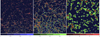 |
Fig. 6. Luminosity density fields in 400 × 400 × 1 h−1 Mpc slices at identical z−coordinates of the central region of the SDSS sample, smoothed with kernels of radii 1, 2, and 8 h−1 Mpc (left, middle, and right panels). This figure illustrates the effect of the smoothing length to geometrical properties of clusters and voids. Densities are expressed in logarithmic scale in interval 0.005–15 in mean density units. The colour code is identical in all panels. |
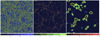 |
Fig. 7. Density fields in 256 × 256 × 0.5 h−1 Mpc slices of the L256 model at identical z-coordinates. Left panel: density field smoothed with the kernel of radius 1 h−1 Mpc in density interval 0.005–15 in mean density units; the colour code below corresponds to this field. Middle panel: same density field in density interval 1.5–15 in mean density units. Faint filaments between high-density knots are invisible. Right panel: field smoothed with kernel 8 h−1 Mpc in interval 1.5–15 in mean density units. Filaments are thicker and percolate easier. In all panels densities are expressed in logarithmic scale. |
The percolation of SDSS samples occurs at lower threshold density than expected from the comparison with DM model samples. In comparison to DM clusters, filling factor functions of SDSS clusters are shifted: cluster filling factors are lower and void filling factors higher. At lowest threshold densities filling factors of DM clusters are close to 1 for all smoothing lengths. In contrast, filling factors of SDSS clusters are much lower, i.e. only ℱC(0.1) = 0.025 for the smoothing kernel RB = 1.
It is remarkable that the number of L512 and SDSS clusters at smoothing length RB = 8 h−1 Mpc reaches maximal values at Dt ≈ 5, and that the number of clusters is also approximately the same for identical small system elimination threshold Nlim = 500. The smoothing length RB = 8 h−1 Mpc and the threshold density Dt ≈ 5 are often used to find superclusters of galaxies (Liivamägi et al. 2012). Samples L512 and SDSS have approximately the same total volumes, thus the close number of superclusters in both samples shows that the L512 model represents the real cosmic web on supercluster level very well.
4.2. Isolated clusters and the separation of intrinsic and selection effects
A further difference of DM and SDSS samples lies in the number functions of clusters for various smoothing lengths. Figure 2 shows that, for smoothing lengths 1, 2, 4 h−1 Mpc and Dt ≤ 4, the number of clusters of SDSS samples is almost independent of the threshold density. Only the sample SDSS.8 has a cluster number function, similar to the number functions of DM samples: a small number of clusters at low threshold density and an increasing number with increasing Dt.
At very low threshold density, Dt = 0.1, the DM samples have one large cluster (NC(0.1) = 1), filling almost the whole space, ℱC(0.1) ≈ 1; see Fig. 2. In Fig. 7 we show the highresolution density field of the L256.1 sample. The left panel shows the density field, smoothed with 1 h−1 Mpc kernel, and plotted in logarithmic scale in density interval 0.005–15 in mean density units. The large DM cluster contains numerous small- and medium-sized knots. The knots of the DM density field are joined to a single high-density region (cluster) by low-density DM filaments and sheets. These faint DM filaments and sheets isolate numerous small voids – bubbles in the high-density matter. For this reason the number of voids in DM samples at low threshold densities is high.
When we increase the threshold density to Dt = 1.5, shown in the middle panel of Fig. 7, then faintest DM filaments between high-density knots are counted as low-density regions. At this density threshold most small knots in the DM density field become isolated clusters and voids merge. For this reason the number of high-density systems (DM clusters) increases with the increase of the threshold density, the number of voids in DM samples decreases, and the lengths of the largest voids increase. We note that the general character of the high-resolution DM density field in the middle panel of Fig. 7 is very similar to the SDSS density field shown in the left panel of Fig. 6.
If we use the largest smoothing kernel, RB = 8 h−1 Mpc, shown in right panels of Figs. 6 and 7, then many previously small clusters join to larger clusters, and the number of clusters decreases. This effect is observed in DM models of all sizes and in the observational SDSS sample. The general character of DM and SDSS density fields at this smoothing kernel is also very similar.
To understand better the nature of this effect, we compare the numbers and diameters of clusters of the DM model sample L512.2 with the numbers and diameters of clusters of the observed sample SDSS.2. The diameters of individual clusters as functions of the distance from the observer are shown in Fig. 8 for the threshold density, Dt = 0.832, and the percolating threshold density of the L512.2 sample, Dt = 3.80. The top panels show the model sample L512.2 and bottom panels show the observed sample SDSS.2.
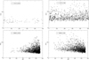 |
Fig. 8. Top: diameters of clusters versus x-coordinate of the sample L512.2, at threshold densities Dt = 0.832, 3.80, left and right panels, respectively. Bottom: diameters of clusters vs. distance from the observer for the SDSS.2 sample at the same threshold densities. Diameters and distances (x-coordinates) are given in h−1 Mpc; diameters are plotted in a logarithmic scale. Largest percolating clusters are not shown. In all samples a small cluster exclusion limit, Nlim = 500, is applied. |
At very low threshold densities the model sample L512.2 has no isolated clusters: the whole over-density region contains one percolating cluster. At the threshold density, Dt = 0.832, the sample L512.2 has one large percolating cluster and about 60 small isolated clusters, i.e. the peaks of the DM density field in low-density regions. These clusters are distributed evenly with distance, and have diameters ~25 h−1 Mpc.
The observed sample SDSS.2 has an approximately constant cluster number function, NC(Dt), at low and medium threshold densities as seen in Fig. 2. The distribution of cluster diameters with distance, shown in Fig. 8 for Dt = 0.832, is very similar at small and medium threshold densities, Dt ≤ 1. At these threshold densities SDSS clusters are isolated and almost identical at different threshold density levels, and for smoothing kernels RB = 1, 2 h−1 Mpc; compare left and middle panels of Fig. 6. Cluster positions and diameters fluctuate slightly because of the inclusion of fainter cluster envelopes by decreasing threshold density. Figure 8 shows that the number of SDSS.2 clusters increases rapidly with the distance from the observer; maximal diameters also increase with distance. Partly this effect is from the conical geometry of the SDSS sample: the volume of the sample increases with distance. But the large number of clusters in SDSS samples is mainly caused by the absence of faint galaxy filaments joining high-density knots at low threshold density to a connected system; see Fig. 6. Moreover, the SDSS sample is flux limited, and at large distance fainter galaxies are not visible, which causes a further increase of the number of large clusters at greater distance from the observer.
Figure 8 shows that at the percolating threshold density of the L512.2 sample, Dt = 3.80, the general trend of diameter distributions of L512.2 and SDSS.2 samples is fairly similar, if we ignore differences due to the conical shape of the SDSS.2 sample. At this threshold density almost all high-density regions of both samples are considered as isolated clusters and have thus a similar character.
When we use the smoothing length 8 h−1 Mpc, the number density function NC of the SDSS sample has a shape, similar to the shape for the L512 sample, as seen in Fig. 2. This means that additional smoothing restores bridges between high-density knots of the SDSS sample, which leads to the loss of most isolated clusters at small threshold densities; see also right panel of Fig. 6.
Void distributions at low threshold densities are very different in model and real samples. Model samples have at these thresholds and at small smoothing lengths numerous small isolated void bubbles and one percolating void. The SDSS sample has only one percolating void and no small voids at all.
But the change of the smoothing scale affects the cluster lengths and numbers of clusters in a different way. Smoothing with 4 h−1 Mpc kernel restores the filamentary character of the SDSS density field (see the next subsection), as characterised by the length of the largest cluster, but not the elimination of small isolated clusters. This means that at the smoothing scale 4 h−1 Mpc and the threshold density Dt = 0.832, there is one large percolating cluster, but numerous small isolated clusters remain. Larger smoothing joins these isolated clusters to the dominating cluster.
The elimination of small isolated clusters at low threshold densities with 8 h−1 Mpc smoothing, but not with 4 h−1 Mpc smoothing suggests that peaks of the SDSS density field are quasi-regularly located with mutual distances of the same order, along the filamentary web. If peaks were randomly located, then the decrease of the number of isolated clusters would be more gradual. An independent confirmation of this result comes from the study by Jõeveer et al. (1978), who found that clusters and groups of galaxies of the Perseus-Pisces supercluster form a long chain with mutual distance between clusters (groups) of ~8 h−1 Mpc. This result was confirmed by a recent study of Tempel et al. (2014a), who demonstrated that galaxy filaments are like pearl necklaces in which groups form density enhancements at a mutual distance ≈7 h−1 Mpc from each other.
These differences in percolation functions and cluster diameter distributions between model and observed samples are caused by two separate effects. The main effect is due to the absence of very faint filamentary systems in the observed sample that is present in DM models. The second effect is caused by selections. The SDSS sample is conical and, at a large distance from the observer, faint galaxies are not included into the sample, which makes faint galaxy filaments, connecting high-density knots, invisible.
The analysis of the distribution of isolated clusters shows that percolation functions are sensitive not only to general geometrical properties of the cosmic web, but also to the presence of faint filaments between high-density knots and to the regular displacement of high-density knots of the web. The analysis also shows that it is relatively easy to separate intrinsic and selection effects in percolation functions.
4.3. Filamentary character of the cosmic web
As seen in Fig. 2, largest clusters of DM samples have for threshold density Dt ≤ P identical percolating lengths, ℱC(Dt) 1, and a very rapid decrease of the length with the increase of the threshold density at Dt > P. This rapid decrease of the length with increasing Dt is characteristic in a filamentary web. The percolation threshold depends on the smoothing length. The smoothing decreases density contrast, thus for larger smoothing lengths percolation occurs at lower threshold densities. In all cases percolation occurs at thresholds much larger than the percolation threshold for a random sample, PC0 = 1.06. Voids of DM samples have similar behaviour. At threshold densities Dt < P void lengths decrease rapidly with decreasing Dt. The DM void percolation thresholds, PV, are much lower than void percolation thresholds for random samples, PV0 = 0.94.
It should be noted that the filamentary character is related to two aspects of the distribution: a rapid change of the length of largest clusters and voids with changing density threshold and a deviation of the respective threshold from the threshold for random samples. The larger this deviation the more filamentary the web is. In a random density field the length of largest clusters (voids) also changes rapidly with the change of the threshold density (see Fig. 1), but the threshold density difference condition is not observed.
The behaviour of length functions of observed samples is different from the behaviour of DM model samples. To see differences between model and observed samples, we compare in Fig. 2 length functions of SDSS and L512 samples at various smoothing lengths. For smoothing kernel RB = 1 h−1 Mpc the largest cluster of the SDSS.1 sample at lowest threshold density Dt = 0.1 has a length ℒC ≈ 0.6, thus the SDSS.1 cluster sample does not percolate at all, and the sample has a meatball type of galaxy distribution. At larger threshold densities maximal length of clusters decreases slowly with increasing Dt.
For smoothing length RB = 2 h−1 Mpc the largest cluster of the SDSS.2 sample percolates at the threshold density PC = 0.2, much lower than the percolation threshold density for random samples, PC0 = 1.06, and for the DM sample L512.2. This means that at this smoothing length the SDSS.2 sample is still mainly a sample of isolated high-density regions, as seen in the middle panel of Fig. 6. But the SDSS.2 sample has also a differential luminosity selection effect. At a smaller distance from the observer, fainter galaxies lie within the observational window of apparent magnitudes and a weak filamentary system of galaxies between high-density knots is present, as seen from Fig. 6. At larger distance from the observer this weak filamentary character of the SDSS.2 sample breaks down. This change of the character of the web influences the length function. The volume of the nearby region, where percolation is easier, is much smaller than the volume of the more distant region. For this reason, in the sample SDSS.2 as a whole a meatball type of the galaxy distribution dominates.
At smoothing lengths 4 and 8 h−1 Mpc the behaviour of the SDSS cluster length functions ℒC(Dt) at large threshold density is almost similar to the behaviour of this function in the DM L512 sample; there is a rapid decrease of the cluster length with increasing threshold, as seen in Fig. 2. However, near to the percolation threshold the change of the cluster length with changing Dt is slower than in a DM model of the same smoothing scale. Thus the percolation of SDSS samples occurs at lower threshold density than expected from the DM sample with similar smoothing scales, L512.4 and L512.8. In model samples the rapid increase of the length of clusters near to the percolation threshold is fostered by the presence of filaments nearby knots. In the SDSS sample at large distance filaments are weaker, thus a bit lower threshold density is needed to get the maximal length of the cluster, equal to the characteristic length of the sample, L0. If this deviation of the SDSS length function near to the percolation threshold is ignored and the length functions of SDSS samples are interpolated up to the percolation threshold in a way similar to the L512 samples, we get for the percolation threshold of SDSS.4 and SDSS.8 values, very close to values for DM samples L512.4 and L512.8. Figure 6 shows that at smoothing scale 8 h−1 Mpc the filamentary character of the SDSS sample is practically restored over the whole depth of the SDSS sample.
4.4 Fatness factors of clusters and voids
General geometrical properties of the cosmic web can be studied using Minkowski functionals; for pioneering papers see Mecke et al. (1994), Sathyaprakash et al. (1998a), and Schmalzing et al. (1999). Minkowski functionals can be used to calculate their combinations as shapefinders: i.e. the thickness, breadth, and length of clusters, as done by Sahni et al. (1998), Sheth et al. (2003), and Shandarin et al. (2004).
In this paper we define a new shape parameter of clusters and voids, the fatness factor: the ratio of the volume of clusters and voids to the maximal possible volume for a given diameter, (5)
(5)
where  is the mean diameter of the cluster along x, y, z axes and V is the volume of the cluster. A similar definition is used to calculate fatness factors of voids.
Fatness factors are dimensionless quantities and describe the fragile shape of clusters and voids. Clusters percolate at threshold density Dt ≈ 5, and fill only about ℱC(P) ≈ 10−3 of space (for smoothing scale 1 h−1 Mpc). This means that clusters at percolation thresholds are extended multi-branching lowvolume and fragile structures in all directions. With the decrease of threshold density the volume of clusters increases and their fragility decreases. Fragile clusters and voids are illustrated in Figs. 14–17 by Shandarin et al. (2004).
In top panels of Fig. 9 we present fatness factors of all clusters and voids of the DM L512.1 sample at percolation thresholds Df = 5.01 and Dt = 0.126, respectively. Fatness factors are shown as functions of volumes of clusters, V, expressed in cubic h−1 Mpc. A similar presentation was given by Shandarin et al. (2006) for shapes and volumes of voids in their analysis of the CDM model. These authors used the term porosity to denote the fragile shape of systems. We see that fatness factors of largest clusters are TC ≈ 10−3, whereas fatness factors of largest voids are TV ≈ 10−1.
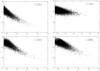 |
Fig. 9.
Top: fatness factors, |

The bottom panels of Fig. 9 show the role of smoothing to fatness factors. The bottom left panel shows fatness factors of the L512.2 sample at percolation threshold Dt = 3.80, and the bottom right panel indicates the fatness factors of the SDSS.2 samples at the same threshold. Largest clusters of both samples have fatness factors, TC ≈ 10−2. In all samples the mean fatness factor decreases with the increase of the volume of clusters and voids. This decrease is larger in cluster samples obtained with smaller smoothing length and smaller in void samples. The maximal possible value of the fatness factor has a system, filling the whole possible cubic space for a given diameter, T = 1.0. A spherical system has the fatness factor, T = π/6 = 0.524. Figure 9 shows that smallest clusters of samples L512.2 and SDSS.2 have mean fatness factors around this value.
We define fatness factor functions, T (Dt), as follows: fatness factors of the largest clusters (voids) as functions of the threshold density. Fatness factor functions are shape functions of the cosmic web. Figure 10 shows fatness factor functions of the largest clusters and voids of the L512 model (left), and of the SDSS galaxy sample (right). Fatness factor functions are calculated for smoothing lengths RB = 1, 2, 4, 8 h−1 Mpc. At a high threshold density the largest clusters are relatively small systems, their fatness factors fluctuate around 10−2. Fatness factors have smallest values near to the percolation threshold density. Below the percolation threshold density cluster fatness factors start to grow, due to the growth of cluster filling factors. Further lowering the threshold density leads to additional cluster merging and the volume of the largest cluster increases continuously. Thus fatness factors of clusters grow and reach values close to unity at the smallest threshold densities. The largest cluster fills almost the whole volume of the sample. In the threshold density range in which clusters (voids) are percolated, diameters of clusters (voids) are equal to their maximal length, Dm = L0, thus in this range T (Dt) = ℱ (Dt).
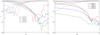 |
Fig. 10. Fatness factor functions, T (Dt), of largest clusters and voids of the L512 model (left) and of the SDSS galaxy sample (right). Functions for clusters are shown by solid lines and are indicated for voids by dashed lines. |
Fatness factor functions of voids of L512 model samples have similar behaviour, when started from low threshold densities. At low threshold densities the largest voids are isolated and their fatness factors fluctuate around the value 10−1. At void percolation threshold density void volumes start to grow continuously and the fatness factor function grows towards unity, following the filling factor function.
The behaviour of the fatness factor functions of SDSS clusters is different from the behaviour of similar functions of model clusters. At all smoothing lengths fatness factors of SDSS clusters at low threshold densities are smaller than fatness factors of L512 model clusters. This difference is because at small threshold densities model clusters include their volume low-density filaments and sheets of DM, which are not present as galaxy filaments in SDSS samples. Fatness factor functions of SDSS voids are very different from fatness factor functions of L512 voids. Voids in SDSS samples are percolating at all threshold densities and cover large volumes. Thus filling factor and fatness functions of SDSS voids are always large, especially for small smoothing lengths.
5. Discussion and summary
5.1. Percolation method as a cosmological tool
The percolation method can be applied in two ways. A simple application is to use it as a tool to select certain kind of galaxy systems from the density field. In this role it was used by Einasto et al. (2006, 2007), Liivamägi et al. (2012), and Einasto (2017) to find superclusters of galaxies for further detailed analysis. Another example is provided by Shandarin et al. (2006), who selected voids in a CDM model and studied their shapes and sizes. In this paper we selected clusters and voids of the density field and investigated their distributions and fatness properties.
The second possibility is to use the percolation method as a tool to investigate geometrical properties of the cosmic web. The extended percolation analysis as used in this paper is sensitive not only to the connectivity of highand low-density regions, but to a number of other geometrical properties of the web as well. Among these properties are the presence or absence of faint filaments around high-density knots, the filamentary character of the web, the deviation of the density field from the Gaussian field, and the main topological type of the web. The extended percolation analysis allows us to calculate a large number of functions that characterise the general geometrical properties of the density field. It also allows us to define important quantitative parameters, such as the percolation threshold density. This parameter depends on the smoothing length that is used in the calculation of the density field.
To judge the quality of the percolation method to investigate the structure of the cosmic web, we have to know how sensitive it is to various basic parameters of the model such as the cosmology, given by the power spectrum of density fluctuations, used to simulate the cosmic web and the size of the simulation box. The CDM model is now well established, thus we see no need to vary cosmological parameters. Instead we calculated percolation functions for DM simulations in four box sizes from 100 to 1024 h−1 Mpc with identical resolutions 5123 particles and cells. This test showed that percolation functions of models of different sizes are very similar to each other. This stability suggests that properties of the cosmic web, as found in the present paper, can be applied to the cosmic web as a whole. Differences due to the use of several independent realisations of the model are much smaller than with different box sizes.
Errors of percolation functions can be estimated on the basis of the shape of these functions. In this paper we are interested essentially in general geometrical properties of the cosmic web as an ensemble, thus exact errors of these functions are of minor importance. We calculated errors only for percolation density thresholds and for filling factors at mean threshold density, Dt = 1. Our analysis has shown that these errors are surprisingly small.
The most significant effect in percolation functions is due to the use of different smoothing scales. To estimate the influence of this effect, we used four values of the smoothing kernel radius. In this way the effect is well known. This sensitivity shows that different samples can be compared only using identical smoothing scales. We consider DM as a physical fluid having continuous density distribution. The fine structure of the DM is seen inside DM haloes, which have a characteristic size of 1 h−1 Mpc. When we investigate the structure of the cosmic web, then fine details of the web within galaxy or cluster sized haloes and filaments are not important. For this reason we consider the smoothing length RB = 1 h−1 Mpc as representing the true density field of the web. To get a complex picture of properties of the cosmic web, the use of different smoothing scales is needed.
At small smoothing scale geometrical properties of clusters and voids are asymmetrical. A symmetry of properties of clusters and voids, observed in several studies (Gott et al. 1986), is valid only when a large smoothing is applied.
Our study has shown that at low threshold densities, Dt ≤ 0.5, percolation functions are very sensitive to the presence or absence of faint filaments between high-density knots. In this threshold density interval the fine structure of clusters and voids of model and real samples are very different. It is clear that the high sensitivity of the extended percolation method to the filamentary character of faint features of the web can help to investigate the bias between galaxy and matter distributions.
At medium threshold densities, 0.5 < Dt < 3, percolation functions depend on the true density distribution and on observational selection effects. Difficulties in the use of flux-limited observational samples were mentioned by Martínez & Saar (2002) in the discussion of percolation functions. This could be the reason why percolation analysis has been made so far mostly for DM models only. Our discussion of this effect has shown that the influence of selection effects to percolation properties is well understood, and we can get valuable information on clustering properties of the cosmic web by comparing DM models with observations.
At high threshold densities, Dt ≥ 3, percolation properties of DM model clusters are approximately similar to percolation properties of SDSS cluster samples. One interesting detail is that percolation functions depend not only on general geometry of the density distribution, but also on the filamentary character of the web and on the location of knots in filaments.
5.2. Summary remarks
Our work has shown that the extended percolation analysis is a versatile method to study various geometrical properties of the cosmic web in a wide range of parameters. We can highlight our findings as follows:
-
Percolation functions of CDM models of sizes from 100 to 1024 h−1 Mpc are very similar to each other. This stability suggests that properties of the cosmic web, as found in the present paper, can be applied to the cosmic web as a whole.
-
The percolation threshold of DM models is a function of the smoothing length, RB. The percolation threshold of DM clusters is log PC = 0.718 − 0.444 × log RB, and of DM voids is log PV = −0.816 + 0.503 × log RB, which differs from percolation threshold of random samples, log P0 = 0.00 ± 0.02.
-
Percolation functions depend on the smoothing length to calculate density fields. Very small smoothing characterises the fine structure inside haloes and large smoothing shifts part of matter from high-density regions to their surroundings.
-
Percolation functions are sensitive to very faint filaments of the cosmic web that are present in DM models, but absent in SDSS samples. At low and medium threshold densities, and at smoothing length ~1 h−1 Mpc, percolation functions of the SDSS sample are different from percolation functions of DM model samples, both for clusters and voids. The SDSS sample has only one large percolating void, which fills almost the whole volume and contains numerous isolated clusters at low threshold densities that are absent in model samples. At large threshold densities percolation properties of DM and SDSS clusters are similar.
-
Percolation analysis allows us to calculate fatness of clusters and voids: the ratio of the volume of clusters (voids) to their maximal possible value. Near percolation threshold the fatness of DM clusters is ≈10−3, and of DM voids ≈10−1.
Differences between distributions of galaxies in the real world and particles in numerical models were discussed in early papers (Jõeveer et al. 1978; Zeldovich et al. 1982; Peebles 2001). The extended percolation analysis describes these differences in a complex way. The application of the extended percolation method to a more detailed investigation of the formation of the cosmic web is an interesting goal for future studies.
Acknowledgments
We thank Gert Hütsi, Mirt Gramann, Antti Tamm, and Elmo Tempel for discussions and the anonymous referee for useful suggestions. We give special thanks to Enn Saar, who developed the very efficient code to find over- and under-density regions. This work was supported by institutional research funding IUT26-2 and IUT40-2 of the Estonian Ministry of Education and Research. We acknowledge the support by the Centre of Excellence “Dark side of the Universe” (TK133) financed by the European Union through the European Regional Development Fund. The study has also been supported by ICRAnet through a professorship for Jaan Einasto. We thank the SDSS Team for the publicly available data releases. Funding for the SDSS and SDSS-II has been provided by the Alfred P. Sloan Foundation, the Participating Institutions, the National Science Foundation, the U.S. Department of Energy, the National Aeronautics and Space Administration, the Japanese Monbukagakusho, the Max Planck Society, and the Higher Education Funding Council for England. The SDSS Web Site is http://www.sdss.org/. The SDSS is managed by the Astrophysical Research Consortium for the Participating Institutions. The Participating Institutions are the American Museum of Natural History, Astrophysical Institute Potsdam, University of Basel, University of Cambridge, Case Western Reserve University, University of Chicago, Drexel University, Fermilab, the Institute for Advanced Study, the Japan Participation Group, Johns Hopkins University, the Joint Institute for Nuclear Astrophysics, the Kavli Institute for Particle Astrophysics and Cosmology, the Korean Scientist Group, the Chinese Academy of Sciences (LAMOST), Los Alamos National Laboratory, the Max-Planck-Institute for Astronomy (MPIA), the Max-Planck-Institute for Astrophysics (MPA), New Mexico State University, Ohio State University, University of Pittsburgh, University of Portsmouth, Princeton University, the United States Naval Observatory, and the University of Washington.
References
- Aihara, H., Allende Prieto, C., An, D., et al. 2011, ApJS, 193, 29 [NASA ADS] [CrossRef] [Google Scholar]
- Aragon-Calvo, M. A., & Szalay, A. S. 2013, MNRAS, 428, 3409 [NASA ADS] [CrossRef] [Google Scholar]
- Aragon-Calvo, M. A., Jones, B. J. T., van de Weygaert, R., & van der Hulst, J. M. 2007, A&A, 474, 315 [NASA ADS] [CrossRef] [EDP Sciences] [Google Scholar]
- Aragon-Calvo, M. A., van de Weygaert, R., Araya-Melo, P. A., Platen, E., & Szalay, A. S. 2010a, MNRAS, 404, L89 [NASA ADS] [CrossRef] [Google Scholar]
- Aragon-Calvo, M. A., van de Weygaert, R., & Jones, B. J. T. 2010b, MNRAS, 408, 2163 [NASA ADS] [CrossRef] [Google Scholar]
- Bertschinger, E. 1995, ArXiv e-prints [arXiv:astro-ph/9506070] [Google Scholar]
- Boerner, G., & Mo, H. 1989, A&A, 224, 1 [NASA ADS] [Google Scholar]
- Bond, J. R., Kofman, L., & Pogosyan, D. 1996, Nature, 380, 603 [NASA ADS] [CrossRef] [Google Scholar]
- Cautun, M., van de Weygaert, R., & Jones, B. J. T. 2013, MNRAS, 429, 1286 [NASA ADS] [CrossRef] [Google Scholar]
- Cautun, M., van de Weygaert, R., Jones, B. J. T., & Frenk, C. S. 2014, MNRAS, 441, 2923 [NASA ADS] [CrossRef] [Google Scholar]
- Colberg, J. M., Pearce, F., Foster, C., et al. 2008, MNRAS, 387, 933 [NASA ADS] [CrossRef] [Google Scholar]
- Dominik, K. G., & Shandarin, S. F. 1992, ApJ, 393, 450 [NASA ADS] [CrossRef] [Google Scholar]
- Einasto, J. 2017, ASP Conf. Ser., 511, 141 [Google Scholar]
- Einasto, J., & Gramann, M. 1993, ApJ, 407, 443 [NASA ADS] [CrossRef] [Google Scholar]
- Einasto, J., & Saar, E. 1987, in Observational Cosmology, eds. A. Hewitt, G. Burbidge, & L. Z. Fang, IAU Symp., 124, 349 [Google Scholar]
- Einasto, J., Kaasik, A., & Saar, E. 1974, Nature, 250, 309 [NASA ADS] [CrossRef] [Google Scholar]
- Einasto, J., Jõeveer, M., & Saar, E. 1980, MNRAS, 193, 353 [NASA ADS] [CrossRef] [Google Scholar]
- Einasto, J., Klypin, A. A., Saar, E., & Shandarin, S. F. 1984, MNRAS, 206, 529 [NASA ADS] [CrossRef] [Google Scholar]
- Einasto, J., Gramann, M., Einasto, M., et al. 1986, Estonian Acad Sci., Preprint, A-9, 3 [Google Scholar]
- Einasto, J., Einasto, M., & Gramann, M. 1989, MNRAS, 238, 155 [NASA ADS] [Google Scholar]
- Einasto, J., Einasto, M., Hütsi, G., et al. 2003, A&A, 410, 425 [NASA ADS] [CrossRef] [EDP Sciences] [Google Scholar]
- Einasto, J., Einasto, M., Saar, E., et al. 2006, A&A, 459, L1 [NASA ADS] [CrossRef] [EDP Sciences] [Google Scholar]
- Einasto, J., Einasto, M., Tago, E., et al. 2007, A&A, 462, 811 [NASA ADS] [CrossRef] [EDP Sciences] [Google Scholar]
- Einasto, M., Tago, E., Lietzen, H., et al. 2014, A&A, 568, A46 [NASA ADS] [CrossRef] [EDP Sciences] [Google Scholar]
- Falck, B., & Neyrinck, M. C. 2015, MNRAS, 450, 3239 [NASA ADS] [CrossRef] [Google Scholar]
- Gott, J. R., III, Dickinson, M., & Melott, A. L. 1986, ApJ, 306, 341 [NASA ADS] [CrossRef] [Google Scholar]
- Gregory, S. A., & Thompson, L. A. 1978, ApJ, 222, 784 [NASA ADS] [CrossRef] [Google Scholar]
- Huchra, J. P., & Geller, M. J. 1982, ApJ, 257, 423 [NASA ADS] [CrossRef] [Google Scholar]
- Jõeveer, M., & Einasto, J. 1977, Estonian Acad. Sci. Preprint, 3 [Google Scholar]
- Jõeveer, M., & Einasto, J. 1978, in Large Scale Structures in the Universe, eds. M. S. Longair, & J. Einasto, IAU Symp., 79, 241 [Google Scholar]
- Jõeveer, M., Einasto, J., & Tago, E. 1978, MNRAS, 185, 357 [NASA ADS] [CrossRef] [Google Scholar]
- Jones, B. J. T., Martinez, V. J., Saar, E., & Einasto, J. 1988, ApJ, 332, L1 [NASA ADS] [CrossRef] [Google Scholar]
- Karachentsev, I. D., Sharina, M. E., Makarov, D. I., et al. 2002, A&A, 389, 812 [NASA ADS] [CrossRef] [EDP Sciences] [Google Scholar]
- Klypin, A., & Shandarin, S. F. 1993, ApJ, 413, 48 [NASA ADS] [CrossRef] [Google Scholar]
- Klypin, A., Kravtsov, A. V., Valenzuela, O., & Prada, F. 1999, ApJ, 522, 82 [Google Scholar]
- Libeskind, N. I., van de Weygaert, R., Cautun, M., et al. 2018, MNRAS, 473, 1195 [NASA ADS] [CrossRef] [Google Scholar]
- Liivamägi, L. J., Tempel, E., & Saar, E. 2012, A&A, 539, A80 [NASA ADS] [CrossRef] [EDP Sciences] [Google Scholar]
- Mandelbrot, B. B. 1982, in The Fractal Geometry of Nature (San Francisco: Freeman) [Google Scholar]
- Martínez, V. J., & Saar, E. 2002, in Statistics of the Galaxy Distribution (Chapman & Hall/CRC) [Google Scholar]
- Mecke, K. R., Buchert, T., & Wagner, H. 1994, A&A, 288, 697 [NASA ADS] [Google Scholar]
- Melott, A. L., Einasto, J., Saar, E., et al. 1983, Phys. Rev. Lett., 51, 935 [NASA ADS] [CrossRef] [Google Scholar]
- Mo, H. J., & Boerner, G. 1990, A&A, 238, 3 [NASA ADS] [Google Scholar]
- Peebles, P. J. E. 2001, ApJ, 557, 495 [NASA ADS] [CrossRef] [Google Scholar]
- Sahni, V., Sathyaprakash, B. S., & Shandarin, S. F. 1997, ApJ, 476, L1 [NASA ADS] [CrossRef] [Google Scholar]
- Sahni, V., Sathyaprakash, B. S., & Shandarin, S. F. 1998, ApJ, 495, L5 [NASA ADS] [CrossRef] [Google Scholar]
- Sathyaprakash, B. S., Sahni, V., & Shandarin, S. 1998a, ApJ, 508, 551 [NASA ADS] [CrossRef] [Google Scholar]
- Sathyaprakash, B. S., Sahni, V., Shandarin, S., & Fisher, K. B. 1998b, ApJ, 507, L109 [NASA ADS] [CrossRef] [Google Scholar]
- Schmalzing, J., Buchert, T., Melott, A. L., et al. 1999, ApJ, 526, 568 [NASA ADS] [CrossRef] [Google Scholar]
- Shandarin, S. F. 1983, Pisma v Astronomicheskii Zhurnal., 9, 195 [Google Scholar]
- Shandarin, S. F., Sheth, J. V., & Sahni, V. 2004, MNRAS, 353, 162 [NASA ADS] [CrossRef] [Google Scholar]
- Shandarin, S., Feldman, H. A., Heitmann, K., & Habib, S. 2006, MNRAS, 367, 1629 [NASA ADS] [CrossRef] [Google Scholar]
- Sheth, J. V., Sahni, V., Shandarin, S. F., & Sathyaprakash, B. S. 2003, MNRAS, 343, 22 [NASA ADS] [CrossRef] [Google Scholar]
- Sorce, J. G., Gottlöber, S., Yepes, G., et al. 2016, MNRAS, 455, 2078 [NASA ADS] [CrossRef] [Google Scholar]
- Springel, V. 2005, MNRAS, 364, 1105 [NASA ADS] [CrossRef] [Google Scholar]
- Stauffer, D. 1979, Phys. Rep., 54, 1 [NASA ADS] [CrossRef] [Google Scholar]
- Sutter, P. M., Lavaux, G., Hamaus, N., et al. 2015, Astronomy Comput., 9, 11 [NASA ADS] [CrossRef] [Google Scholar]
- Tago, E., Saar, E., Tempel, E., et al. 2010, A&A, 514, A102 [NASA ADS] [CrossRef] [EDP Sciences] [Google Scholar]
- Tegmark, M., Strauss, M. A., Blanton, M. R., et al. 2004, Phys. Rev. D, 69, 103501 [CrossRef] [Google Scholar]
- Tempel, E., Einasto, J., Einasto, M., Saar, E., & Tago, E. 2009, A&A, 495, 37 [NASA ADS] [CrossRef] [EDP Sciences] [Google Scholar]
- Tempel, E., Tago, E., & Liivamägi, L. J. 2012, A&A, 540, A106 [NASA ADS] [CrossRef] [EDP Sciences] [Google Scholar]
- Tempel, E., Kipper, R., Saar, E., et al. 2014a, A&A, 572, A8 [NASA ADS] [CrossRef] [EDP Sciences] [Google Scholar]
- Tempel, E., Stoica, R. S., Martínez, V. J., et al. 2014b, MNRAS, 438, 3465 [NASA ADS] [CrossRef] [Google Scholar]
- Tempel, E., Tamm, A., Gramann, M., et al. 2014c, A&A, 566, A1 [NASA ADS] [CrossRef] [EDP Sciences] [Google Scholar]
- Tinsley, B. M. 1968, ApJ, 151, 547 [NASA ADS] [CrossRef] [Google Scholar]
- Tully, R. B., Courtois, H., Hoffman, Y., & Pomarède, D. 2014, Nature, 513, 71 [NASA ADS] [CrossRef] [Google Scholar]
- van de Weygaert, R., & Schaap, W. 2009, Lect. Notes Phys., 665, 291 [Google Scholar]
- van de Weygaert, R., Shandarin, S., Saar, E., & Einasto, J. 2016, IAU Symp., 308 [Google Scholar]
- White, S. D. M., & Rees, M. J. 1978, MNRAS, 183, 341 [NASA ADS] [CrossRef] [Google Scholar]
- Yess, C., & Shandarin, S. F. 1996, ApJ, 465, 2 [NASA ADS] [CrossRef] [Google Scholar]
- Yess, C., Shandarin, S. F., & Fisher, K. B. 1997, ApJ, 474, 553 [NASA ADS] [CrossRef] [Google Scholar]
- Zeldovich, Y. B., Einasto, J., & Shandarin, S. F. 1982, Nature, 300, 407 [NASA ADS] [CrossRef] [Google Scholar]
All Tables
All Figures
|
Fig. 1. Change of percolation functions of the model L512 with simulation epoch. Panels from top to bottom are for the initial epoch, z = 30, and epochs z = 10, z = 3, z = 1, and z = 0. Left panels: lengths of largest clusters and voids, ℒ(Dt) = Lmax/L0; centre panels: filling factors of largest clusters and voids, ℱ (Dt) = Vmax/V0; right panels: numbers of clusters and voids, N(Dt); all as functions of the threshold density, Dt. Functions are found for original non-smoothed density fields, which correspond to a resolution 1 h−1 Mpc. Functions for clusters are plotted with solid lines, for voids with dashed lines. |
| In the text | |
|
Fig. 2. Percolation functions of model and observational samples: left panels: lengths of largest clusters and voids, ℒ(Dt) = Lmax/L0; centre panels: filling factors of largest clusters and voids, ℱ (Dt) = Vmax/V0; right panels: numbers of clusters and voids, N(Dt), as functions of the threshold density, Dt. Lengths and filling factors are expressed in units of the total lengths and volumes of samples. Top panels represent the DM model L512; bottom panels represent the SDSS samples. Percolation functions are found using smoothing kernels of radii 1, 2, 4, and 8 h−1 Mpc. Solid lines show data on clusters, and dashed lines on voids. Indices show the smoothing kernel length in h−1 Mpc. Number functions N(Dt) of DM models in this figure correspond to small system excursion limit Nlim = 50 cells. |
| In the text | |
|
Fig. 3. Percolation threshold of clusters and voids, PC and PV, of models L100, L256, L512, L1024 for various smoothing lengths RB. Filled symbols are for clusters, open symbols for voids. Linear fits according to Eq. (3) are shown by solid lines, 95% confidence limits by dashed lines. |
| In the text | |
|
Fig. 4. Filling factors of largest clusters and voids at mean threshold density, ℱC(1) and ℱV(1), of models L100, L256, L512, L1024 for various smoothing lengths RB. Filled symbols indicate clusters; open symbols indicate voids. Linear fits according to Eq. (4) are shown by solid lines, 95% confidence limits by dashed lines. |
| In the text | |
|
Fig. 5. Filling factor functions of the model L512: total filling factors of clusters and voids, ℱtot, and filling factors of maximal clusters and voids, ℱmax, as functions of threshold density, Dt, plotted in logarithmic scales. Solid lines indicate total filling factors of high- and low-density regions, dashed lines indicate maximal clusters and voids, blue indicates clusters, and black indicates voids. Functions are calculated using smoothing kernels 2 and 8 h−1 Mpc (left and right panels). Bottom row: the same functions for observed SDSS samples. |
| In the text | |
|
Fig. 6. Luminosity density fields in 400 × 400 × 1 h−1 Mpc slices at identical z−coordinates of the central region of the SDSS sample, smoothed with kernels of radii 1, 2, and 8 h−1 Mpc (left, middle, and right panels). This figure illustrates the effect of the smoothing length to geometrical properties of clusters and voids. Densities are expressed in logarithmic scale in interval 0.005–15 in mean density units. The colour code is identical in all panels. |
| In the text | |
|
Fig. 7. Density fields in 256 × 256 × 0.5 h−1 Mpc slices of the L256 model at identical z-coordinates. Left panel: density field smoothed with the kernel of radius 1 h−1 Mpc in density interval 0.005–15 in mean density units; the colour code below corresponds to this field. Middle panel: same density field in density interval 1.5–15 in mean density units. Faint filaments between high-density knots are invisible. Right panel: field smoothed with kernel 8 h−1 Mpc in interval 1.5–15 in mean density units. Filaments are thicker and percolate easier. In all panels densities are expressed in logarithmic scale. |
| In the text | |
|
Fig. 8. Top: diameters of clusters versus x-coordinate of the sample L512.2, at threshold densities Dt = 0.832, 3.80, left and right panels, respectively. Bottom: diameters of clusters vs. distance from the observer for the SDSS.2 sample at the same threshold densities. Diameters and distances (x-coordinates) are given in h−1 Mpc; diameters are plotted in a logarithmic scale. Largest percolating clusters are not shown. In all samples a small cluster exclusion limit, Nlim = 500, is applied. |
| In the text | |
|
Fig. 9.
Top: fatness factors, |
| In the text | |
|
Fig. 10. Fatness factor functions, T (Dt), of largest clusters and voids of the L512 model (left) and of the SDSS galaxy sample (right). Functions for clusters are shown by solid lines and are indicated for voids by dashed lines. |
| In the text | |
Current usage metrics show cumulative count of Article Views (full-text article views including HTML views, PDF and ePub downloads, according to the available data) and Abstracts Views on Vision4Press platform.
Data correspond to usage on the plateform after 2015. The current usage metrics is available 48-96 hours after online publication and is updated daily on week days.
Initial download of the metrics may take a while.