| Issue |
A&A
Volume 616, August 2018
|
|
|---|---|---|
| Article Number | A56 | |
| Number of page(s) | 8 | |
| Section | Interstellar and circumstellar matter | |
| DOI | https://doi.org/10.1051/0004-6361/201832935 | |
| Published online | 15 August 2018 | |
Magnetic field in a young circumbinary disk★
1
Max-Planck-Institut für extraterrestrische Physik,
Giessenbachstr. 1,
85748
Garching,
Germany
e-mail: This email address is being protected from spambots. You need JavaScript enabled to view it.
2
Institut de Ciències de l’Espai (ICE), CSIC, Can Magrans s/n, Cerdanyola del Vallès,
08193
Catalonia,
Spain
3
Institut d’Estudis Espacials de Catalunya (IEEC),
08034
Barcelona,
Catalonia,
Spain
4
INAF-Osservatorio Astrofisico di Arcetri,
Largo E. Fermi 5,
50125
Firenze,
Italy
5
Departamento de Física–ICEx–UFMG,
Caixa Postal 702,
30.123-970
Belo Horizonte,
Brazil
6
Department of Earth and Space Sciences, Chalmers University of Technology,
Onsala Space Observatory,
439 92
Onsala,
Sweden
7
Harvard-Smithsonian Center for Astrophysics,
60 Garden Street,
Cambridge,
02138 MA,
USA
8
Max-Planck-Institut für Radioastronomie,
Auf dem Hügel 69,
53121
Bonn,
Germany
Received:
2
March
2018
Accepted:
1
May
2018
Abstract
Context. Polarized continuum emission at millimeter-to-submillimeter wavelengths is usually attributed to thermal emission from dust grains aligned through radiative torques with the magnetic field. However, recent theoretical work has shown that under specific conditions polarization may arise from self-scattering of thermal emission and by radiation fields from a nearby stellar object.
Aims. We use multi-frequency polarization observations of a circumbinary disk to investigate how the polarization properties change at distinct frequency bands. Our goal is to discern the main mechanism responsible for the polarization through comparison between our observations and model predictions for each of the proposed mechanisms.
Methods. We used the Atacama Large Millimeter/submillimeter Array to perform full polarization observations at 97.5 GHz (Band 3), 233 GHz (Band 6) and 343.5 GHz (Band 7). The ALMA data have a mean spatial resolution of 28 AU. The target is the Class I object BHB07-11, which is the youngest object in the Barnard 59 protocluster. Complementary Karl G. Jansky Very Large Array observations at 34.5 GHz were also performed and revealed a binary system at centimetric continuum emission within the disk.
Results. We detect an extended and structured polarization pattern that is remarkably consistent between the three bands. The distribution of polarized intensity resembles a horseshoe shape with polarization angles following this morphology. From the spectral index between Bands 3 and 7, we derived a dust opacity index β ~ 1 consistent with maximum grain sizes larger than expected to produce self-scattering polarization in each band. The polarization morphology and the polarization levels do not match predictions from self-scattering. On the other hand, marginal correspondence is seen between our maps and predictions from a radiation field model assuming the brightest binary component as main radiation source. Previous molecular line data from BHB07-11 indicates disk rotation. We used the DustPol module of the ARTIST radiative transfer tool to produce synthetic polarization maps from a rotating magnetized disk model assuming combined poloidal and toroidal magnetic field components. The magnetic field vectors (i.e., the polarization vectors rotated by 90°) are better represented by a model with poloidal magnetic field strength about three times the toroidal one.
Conclusions. The similarity of our polarization patterns among the three bands provides a strong evidence against self-scattering and radiation fields. On the other hand, our data are reasonably well reproduced by a model of disk with toroidal magnetic field components slightly smaller than poloidal ones. The residual is likely to be due to the internal twisting of the magnetic field due to the binary system dynamics, which is not considered in our model.
Key words: magnetic fields / polarization / scattering / instrumentation: interferometers / techniques: polarimetric / protoplanetary disks
The reduced images as FITS files are only available at the CDS via anonymous ftp to cdsarc.u-strasbg.fr (130.79.128.5) or via http://cdsarc.u-strasbg.fr/viz-bin/qcat?J/A+A/616/A56
© ESO 2018
1 Introduction
Polarized emission of dust grains is considered to be a good tracer of the magnetic field in the interstellar medium, since aspherical dust particles tend to align their short axis parallel to the local direction of the field, with the help of radiative torques (see, e.g., Draine & Weingartner 1997; Andersson et al. 2015). The method has been successfully used to map the morphology of the magnetic field in star forming regions, over scales ranging from molecular clouds (Planck Collaboration Int. XXXV 2016) to protostellar envelopes (e.g., Girart et al. 2006; Alves et al. 2011; Hull et al. 2014; Zhang et al. 2014). Recently, millimeter-wave polarimetry has become sensitive enough to allow us to detect the polarized emission of dust in protostellar and protoplanetary disks (starting from Rao et al. 2014), opening the way to address many open questions concerning the role of magnetic fields in the formation and evolution of circumstellar disks (Lizano & Galli 2015). With the Atacama Large Millimeter/submillimeter Array (ALMA), our knowledge on the polarization properties of young stellar objects (YSO) has increased substantially due to the high sensitivity and angular resolution achievable with this instrument (e.g., Hull et al. 2017a,b; Cox et al. 2018; Lee et al. 2018).
However, the interpretation of millimeter-wave polarization observations of disks is not straightforward, because processes other than just emission by magnetically aligned grains may be at play in environments in which a significant number of large grains is expected to be produced by dust coagulation and the local radiative field is relatively intense. In fact, polarized emission in disks can also be produced by self-scattering of an anisotropic radiation field (Kataoka et al. 2015; Yang et al. 2016a,b) and alignment with the radiation anisotropy (also known as “radiative alignment”, Lazarian & Hoang 2007; Tazaki et al. 2017). The former prevails over magnetic alignment if sufficiently large grains are present, resulting in a high scattering opacity and therefore a high contribution of scattered light in the observed emission; the latter dominates if the grain precession rate induced by radiative torques is faster than the Larmor precession around the magnetic field.
In the case of self-scattering, the polarization angle and degree depend on the grain properties and the system geo- metry: for Rayleigh scattering, the polarization pattern is centro-symmetric for face-on disks, and parallel to the minor axis for inclined disks; in the case of radiative alignment, the polarization is perpendicular to the propagation direction of the radiative flux. In this context, the polarized emission observed at three frequency bands in the HL Tau disk has been interpreted as due to self-scattering at 870 μm, and radiative alignment at 3 mm, with intermediate characteristics at 1.3 mm (Kataoka et al. 2017; Stephens et al. 2017). This example stresses the importance of comparing maps at different wavelengths in order to disentangle the possible different contributions to the observed polarization.
This paper introduces the results obtained from the polarized emission observed at three millimeter-to-submillimeter wavebands in the BHB07-11 disk, a Class I object embedded in the darkest parts of the Pipe Nebula, a quite quiescent complex of interstellar clouds located at a distance of 145 pc from the Sun (Alves & Franco 2007). Only a handful of embedded sources are known in the entire complex, among which BHB07-11 is the youngest member of a protocluster of low-mass YSOs (e.g., Brooke et al. 2007).
An earlier non-polarimetric study of BHB07-11 reports the detection of a bipolar molecular outflow launched beyond the edge of the disk, at a distance of ~90–130 astronomical units (AU) from the rotational axis, where infalling gas lands on the disk (Alves et al. 2017). In this paper, we revisit this object in order to investigate the characteristics of the millimeter polarized emission from its disk.
2 Observations
2.1 ALMA
We used the ALMA in full polarization mode, where all correlations between the linear feeds (X, Y) of each antenna are processed. These correlations include the parallel-hand (XX, YY) and the cross-hand (XY, YX) visibilities from which we obtain the Stokes parameters I, Q and U in the image space. The spectral setup have four spectral windows in Time Domain Mode (TDM, 64 channels with a width of 31.5 kHz), which is optimized for observations of continuum emission. We used the atmospheric windows centered at 97.5 GHz (Band 3), 233 GHz (Band 6) and 343.5 GHz (Band 7).
The Band 3 observations were performed in two execution blocks (EBs) on November 14, 2017. The first EB was ~ 1.7 h long and used 44 antennas from the main array. The second EB was ~2.1 h long and used 46 antennas from the main array. The polarization (and flux) calibrator J1733–1304 was measured to have a peak of polarized intensity of 23.13 ± 0.02 mJy beam−1 and mean position angle of –48.8° (east of north, as for all references to polarization position angle from now on). Although the noise level in the image plane of the calibrator is very low, the uncertainty on the absolute flux density scale is expected to be ~ 10%. The mean polarization fraction of 2.4% is consistent with earlier measurements of this object according to the ALMA calibrator source catalog. The phase calibrator J1700–2610 was observed to have a flux density of 1.6 ± 0.2 Jy, which is consistent with the nearest monitoring observations of this object according to the ALMA catalogue. Bandpass calibration was performed through observations of J1924–2914.
The Band 6 observations were performed on September 19, 2015 using 35 antennas of the array. The total observing time was 3 h divided into three EBs of 1 h each. The absolute flux calibration was obtained with observing scans on Titan, the bandpass calibration with J1924–2914, phase calibration with J1713–2658 and the polarization calibration with J1751+0939. While bandpass and gain calibration were performed individually in each EB, the absolute flux calibration obtained for the first EB was bootstrapped to the phase calibrator in the second and third EBs. After concatenation of the three EBs, the polarization calibration was performed and leakage terms were computed. The peak of polarized intensity of the calibrator is ~ 55 mJy beam−1, with a constant polarization level of ~5.5% and position angle of ~ 5.3°. Despite the source variability at this band (according to the ALMA Calibrator Catalogue), the observed polarization levels are fairly consistent with the values observed during its monitoring. The phase calibrator J1713–2658 was measured to have a flux density of 0.14 ± 0.01 Jy. No entries are found in the ALMA calibrator catalogue for this band that would allow for a flux comparison with respect to the ALMA monitoring observations.
The Band 7 observations were carried out on May 17, 2017 using 45 antennas and two EBs of 2 and 1.5 h, respectively. Each EB was calibrated individually in (amplitude and phase) gains and bandpass, while the concatenated dataset was used for polarization calibration due to the optimized parallactic angle coverage. For these observations, the flux calibrator, J1733–1304, was also used as polarization calibrator. The flux density obtained for the phase calibrator, 0.55 ± 0.06 Jy, is consistent with the ALMA calibrator catalogue. The polarization calibrator has a peak of polarized flux of 15.9 mJy beam−1 and an rms noise level of 0.05 mJy beam−1. The polarized level is ~1.6% and position angle 59°, consistent with previous observations listed in the ALMA catalogue.
This work relies on a multi-frequency analysis of polarization properties. Therefore, in order to ensure that the same spatial scales are being used for comparison in the distinct frequency data, we produced cleaned maps using a uv range that is common for all bands, from 27 to 1310 kλ. The inverse Fourier transform of the uv visibilities produced Stokes parameters (I, Q and U) maps with synthesized beams of 0.22′′ × 0.17′′ (position angle = −61.46°), 0.26′′ × 0.15′′ position angle = −85.65°) and 0.21′′ × 0.18′′ (position angle = −72.79°) for Bands 3, 6, and 7, respectively. This corresponds to a mean spatial resolution of ~ 28.3 AU. The total intensity (Stokes I) maps have a rms noise level of 0.012, 0.15 and 0.52 mJy beam−1 for Bands 3, 6, and 7, respectively. The Stokes Q and U maps reached a noise level of ~0.008 mJy beam−1 in Band 3 and ~ 0.03 mJy beam−1 in Bands 6 and 7. The polarized intensity, computed as  , reached a noise level of ~ 0.01 mJy beam−1 in Band 3 and ~0.05 mJy beam−1 in Bands 6 and 7. For the present work, we adopt a signal-to-noise ratio of five in polarized intensity for all bands in order to produce vector maps.
We applied primary beam correction to account for the decreasing instrument sensitivity away from the center of the primary beam. Our source is well centered in the phase center and no extended polarized emission is detected at scales larger than 5.7′′, which corresponds to approximately one third of the primary beam in Band 7 (the smaller of the three bands).
2.2 VLA
We used the Karl G. Jansky Very Large Array (VLA) to observe the continuum emission at 34.5 GHz (λ ~ 8.7 mm, Ka band) inits most extended configuration. The observations were carried out on December 4 and 10, 2016. The total on-source time was 77 min. The calibration was performed using the standard CASA VLA pipeline. The maps were obtained from the calibrated visibilities using a robust weighting of zero, which provided a synthesized beam of 0.10′′× 0.04′′ with a position angle of 12° (i.e., a spatial resolution of ~10 AU at the Pipe nebula distance). The rms noise of the map is 12 μJy beam−1.
Previous VLA lower angular resolution observations (~ 3′′) at 3.6 cm detected the source VLA 5 near the center of the disk of BHB07-11 (Dzib et al. 2013). The new observations resolved VLA 5 in a binary system, VLA 5a (RA = 17:11:23.1057, Dec = − 27:24:32.818) and VLA 5b, (17:11:23.1017, − 27:24:32.985). The uncertainties on the positions are ≃4 mas. Their flux densities are 0.32 ± 0.03 and 0.23 ± 0.03 mJy, respectively.The two radio sources appear inside the disk, slightly offset from the dust millimeter continuum peaks (Fig. 2).
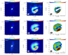 |
Fig. 1 StokesI (left panel), polarized intensity (middle panel), and polarization fraction (right panel) of our Band 3 (upper panels), Band 6 (middle panels), and Band 7 (lower panels) ALMA data. The contours indicate the intensity levels of the Stokes I emission in each band, being 30, 60, 90, 120, 150, and 180 times the rms for bands of 3 and 6 (rmsBand 3 ~ 0.012 mJy beam−1 and rmsBand 6 ~ 0.15 mJy beam−1), and 30, 60, 90, 120 times 0.52 mJy beam−1, the rms for Band 7. The synthesized beams are 0.22′′ × 0.17′′ (position angle = −61.46°) for Band 3, 0.26′′ × 0.15′′ (position angle = −85.65°) for Band 6 and 0.21′′ × 0.18′′ (position angle = −72.79°) for Band 7. The vector map indicates the orientation of the polarization whose length is proportional to the polarization fraction. The vectors are sampled as one vector every two pixels. The two star symbols in the middle-lower panel indicate the position of the two continuum peaks detected in the 34 GHz VLA data, VLA 5a for the northern peak and VLA 5b for the southern one (see also Fig. 2). |
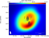 |
Fig. 2 Intensity contours of the 34 GHz VLA emission plotted on top of the Band 7 Stokes I image of BHB07-11. The contours correspond to intensity levels of 3, 5, 7, …, 15, 17 × the noise level of the VLA map, 12 μJy beam−1. The VLA synthesized beam of 0.10′′ × 0.04′′ is shown in the lower left corner. |
3 Polarization properties
The Stokes I continuum emission in the three ALMA bands is consistent with the 1.3 mm continuum map obtained in non- polarimetricmode by Alves et al. (2017). The thermal emission shows the inner envelope, that is, the elongated and tenuous structure that surrounds an at least ten times brighter structure associated with a compact disk of radius ~ 80 AU. The disk brightness shows a strong asymmetry, with enhanced emission toward the southwest.
The polarization properties of the three bands are remarkably similar (Fig. 1). The polarized intensity is spatially confined to the Stokes I emission of the disk. The distribution of polarized intensity and polarization fraction resembles a horseshoe shape peaking in the southwest, similar to the Stokes I emission. The 34 GHz VLA continuum contours are shown with respect to the Stokes I Band 7 emission in Fig. 2. The polarization position angles (PA) have a very similar distribution in all bands (Fig. 3), with the electric field orientation following the structure of the polarized intensity. Interestingly, the polarized intensity increases with total intensity (Fig. 4). Although the polarized intensity is systematically larger for Band 7, the polarization fraction (Ipol ∕Itotal) observed forBand 3 is on average larger than the polarization levels at Bands 6 and 7. Thus, the mean polarization fraction is 7.9% ± 0.8%, 5.3% ± 0.3%, and 3.5% ± 0.1% for Bands 3,6, and 7, respectively. Yet, the spatial distribution of the polarization fraction is very similar in all three bands (right panels of Fig. 1). The polarization fraction exhibit three peaks, with the strongest one offset by ≃ 0.′′1 toward the outer part of the disk with respect to the total intensity peak, located in the southwest region of the disk. This is reflected in Fig. 4, especially for Bands 6 and 7, where points with Stokes I brighter than ~20 and ~ 60 mJy beam−1 have larger polarized intensity levels than the mean polarization fraction. This is likely due to the mismatch between the peak of polarized intensity and total intensity.
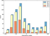 |
Fig. 3 Distribution of polarization angles for each band using a bin of 10°. |
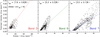 |
Fig. 4 Distribution of the polarized intensity as a function of total intensity. The mean polarization fraction over the regions shown in the right panels of Fig. 1 are indicated in each panel as straight lines. The rms (error bars) for the polarized intensity and total intensity are mentioned in Sect. 2.1. |
4 Spectral properties of the dust emission
Since Bands 3 and 7 have the largest frequency separation among the three bands, we have smoothed the corresponding Stokes I maps to a common beam and used their flux difference to compute the spectral index α as S ∝ να, where S is the intensity and ν is the frequency. Figure 5 shows the spatial distribution of α with respect to Stokes I and polarized intensity. The spectral index has a mean value of 3.01 ± 0.02 with a minimum 2.67 ± 0.01 near the center of the disk. We computed the dust opacity index β assuming an optically thin and Rayleigh−Jeans regime for the disk edge (β = α− 2), and found ⟨β⟩ ~ 1.0, which is within typical values found in in protostellar and YSO disks (e.g., Natta et al. 2007). However, this is lower than the value expected for the interstellar medium (βISM ~ 1.7) and suggests some grain growth, with maximum sizes in the millimeter range (Natta et al. 2007).
An accurate estimation of maximum grain size is affected by departures from the Rayleigh−Jeans regime and changes in optical depth through the disk. Although large, millimeter-size grains have been reported in other circumstellar disks (e.g., Pérez et al. 2015), we cannot discount the effect of optical depth in some regions of BHB07-11. In addition, young Class I disks such as BHB07-11 are expected to have a population of grains significantly smaller than 1 mm, given that recent scattering models have inferred maximum grain sizes of ~ 100 μm in young (Class I/II) protoplanetary disks such as HL Tau (e.g., Kataoka et al. 2016a).
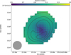 |
Fig. 5 Spectral index map obtained from the Stokes I emission between Bands 3 and 7. The Stokes I maps were smoothed to a common circular beam of 0.25′′ prior to spectral index computation. The contours show the Stokes I Band 7 flux as in Fig. 1. |
5 Origin of polarization
5.1 Investigating whether polarization is produced by self-scattering of dust thermal emission
In the case of a population of grains with different sizes, as expected in the ISM and in protostellar disks, self-scattering is produced by the largest grains, and it has a strong wavelength dependence (Kataoka et al. 2015; Yang et al. 2016a). Thus, the maximum polarization degree is produced in a relatively narrow band around a wavelength of λ ~ 2πamax, where amax is the maximum dust grain size (Kataoka et al. 2016b, 2017), since the polarization degree decreases significantly departing from this frequency for a specificamax. Thus, for example, a population of grains with maximum grain size of 150 μm would produce an averaged polarization degree above 0.5% in the dust emission between roughly 350 μm and 4 mm (values obtained from Fig. 4 of Kataoka et al. 2017). Observations and modeling have revealed that when self-scattering is the dominant mechanism the regions with strongest polarized intensity show typically small polarization levels, <3% (Kataoka et al. 2015; Yang et al. 2017; Girart et al. 2018), although in the edges of the dust emission the polarization can increaseto higher values (e.g., Kataoka et al. 2016b; Girart et al. 2018). In addition, the self-scattering polarization pattern depends basically on the density distribution and disk geometry. The characteristic pattern of the polarization direction is mainly aligned with the disk minor axis (e.g., Kataoka et al. 2016b; Stephens et al. 2017; Hull et al. 2018; Sadavoy et al. 2018). Optical depth effects can affect this pattern, but the mean direction is still aligned withthe minor axis (e.g., Yang et al. 2017). For an intensity distribution with lopsided pattern (such as a transition disk or ring-like disk), the polarization pattern has a clear radial component in the inner part of the ring and an azimuthal component in the outer part of the ring (Kataoka et al. 2015, 2016a). This morphology was confirmed by ALMA observations of HD 142527, a Herbig Ae star surrounded by a protoplanetary disk (Kataoka et al. 2016b).
The observed polarization in the three ALMA bands does not fit the aforementioned properties for self-scattering. First, the observed position angle pattern of the polarization is very different from the one expected for a lopsided disk (Kataoka et al. 2015, 2016a). Second, the polarization degree levels observed in our data (right panels of Fig. 1) are at least a factor of approximately four (in Band 7, higher in Band 3) larger than the total polarization fraction predicted by self-scattering plus radiative alignment in a protoplanetary disk with amax = 150 μm, which is the grain size that contributes more to the modeled polarization (see Fig. 4 in Kataoka et al. 2017). Third, between Bands 3 and 7, the frequency has changed by a factor of 3.5, but the polarization degree has changed by a factor of 2.0, implying that the polarization degree changes more smoothly than expected in the self-scattering model. We therefore rule out self-scattering as potential mechanism to explain our polarization data. Indeed, if the maximum grain size derived from the spectral index analysis is correct (amax ~ millimeter, see Sect. 4), then the highest polarization from self-scattering should occur at wavelengths larger than 1 cm. But at 1 cm the dust peak emission for the measured spectral index would be 73 μJy beam−1. Assuming a 3% polarization degree for self-scattering the polarized intensity would be only few μJy beam−1, which would be only possible to detect with the Next Generation Very Large Array (NGVLA).
Although self-scattering is ruled out to explain our data, other potential mechanisms can still produce the observed polarization. In the following section, we discuss our results in the framework of grain alignment by radiative torques.
5.2 Investigating whether polarization is produced by dust alignment with radiation anisotropy
The dust polarization produced by radiation fields relies on radiative torques imparted on elongated dust grains by an anisotropic radiation field (Lazarian & Hoang 2007). This mechanism is efficient in aligning micrometer-size grains in the interstellar medium with the local magnetic field due to Larmor precession around magnetic field lines. The Larmor precession timescale is inversely proportional to the magnetic field strength and proportional to the dust effective area. This means that for large millimeter-size grains in circumstellar disks, the Larmor precession timescale is longer than the gaseous damping timescale. As a result, the radiative precession of dust grains around the radiation direction will become more efficient and the dust grains will be aligned with the radiative flux rather than the magnetic field.
In this scenario, since the alignment is between the radiation direction and the precession axis (which is perpendicular to the grain long axis), the polarization is perpendicular to the radiation flux gradient, and its overall distribution has a centrosymmetric morphology centered on the source of radiation (Tazaki et al. 2017). In a full disk, the polarized pattern has an azimuthal orien- tation, while for a lopsided disk the polarization pattern is more complicated. However, if the radio sources revealed by the VLA observationsare associated to a proto binary system, they could be a source of anisotropic radiation responsible for aligning grains in the disk.
5.3 Investigating whether polarization is produced by dust alignment with magnetic fields
If Larmor precession prevails over radiative precession, the polarization is produced by thermal emission of elongated grains aligned withthe magnetic field (Andersson et al. 2015). It is well established that the polarization of the millimeter dust emission in dense molecular envelopes surrounding protostars and their disks trace the magnetic field, since the observed field pattern in some cases matches well the theoretical predictions (see, e.g., Girart et al. 2006, 2009; Frau et al. 2011). Therefore, we speculate that being a Class I YSO, the dust grain population in the BHB07-11 disk is not too different from the surrounding envelope feeding the disk.
Upon the assumption that the polarization arises from grain alignment with the magnetic field, the 90°-rotated polarization map shows the plane-of-sky component of the disk magnetic (B) field averaged along the line of sight (Fig. 6). The vector map does not exhibit an obvious azimuthal morphology as previously reported in other young disks seen face-on (e.g., Rao et al. 2014). Instead, the observed pattern could be interpreted as the dragging of the magnetic field lines due to the disk rotation, a precursor of a toroidal B-field morphology.As reported by Alves et al. (2017), the kinematics derived from molecular line observations of BHB07-11 is consistent with infall plus rotation motions at the inner envelope, but it is dominated by Keplerian rotation at scales of ~ 150 AU, corresponding essentially to the disk. Specifically, the H2CO (32,1 − 22,0) emission (ν = 218.760 GHz, Eu ~ 70 K) is confined to the disk in either low and high velocity components (which reach ~ 5.5 km s−1 with respect to the systemic velocity of the object). The velocity centroid map of the molecular emission shows a velocity gradient along the disk long axis (Fig. 6). There is a clear correspondence between the putative B-field lines and the velocity structure.
In the following section, we compare our data with polarization models of radiative alignment and magnetic alignment mechanisms.
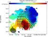 |
Fig. 6 Polarization vectors rotated by 90° showing the plane-of-sky magnetic field configuration at Band 7. Contours show the same Stokes I intensity levels as in Fig. 1. The background image is a moment 1 map of the H2 CO (32,1 − 22,0) emission in BHB07-11. The moment map is produced from a 3σ cut (σ ~ 5.3 mJy beam−1) in the molecular emission. The synthesized beam of the H2CO map is 0.27′′ × 0.21′′. The stars symbols have the same meaning as in Fig. 1. |
6 Polarization models
6.1 Alignment with radiation field
We have built synthetic polarization maps assuming radiation alignment produced by the VLA 5a and VLA 5b sources. We have considered polarization either from each protostar individually or in combination weighted by 1∕d2, where d is the distanceto the protostars. We used the disk inclination and position angle in the plane-of-sky as free parameters. For the scenario where VLA 5b is the main dominant source of radiation, the mean δPA = PAdata − PAmodel is 28.9° with a standard deviation σ of 5.5°. The mean δPA residuals are even larger (>30°) for the model assuming combined radiation from the two protostars. The best fit was achieved in the scenariowhere VLA 5a is the dominant source of radiation, from which a disk inclination of 48° and position angle of 138° were derived (fit error of ± 15°). These values are consistent with our observational estimates (Alves et al. 2017). Figure 7 shows the comparison between our Band 7 polarization maps and the radiation fields polarization produced by VLA 5a, with mean δPA =20.2° and σ =6.9°. However, there is a strong discrepancy in position angles at the northwest portion of the disk. The histogram in Fig. 7 shows the distribution of residuals (δPA) with bins size consistent with the largest observational uncertainty in position angle ( 6°).
6°).
6.2 Alignment with magnetic field
For the case of magnetic alignment, we used the DustPol module of the ARTIST software (Padovani et al. 2012; Jørgensen et al. 2014) to build a disk model including thermal continuum polarization by dust grains aligned by a large-scale magnetic field. In order to model the configuration of the observed magnetic field lines, we assumed the model by Shu et al. (2007) of a viscously accreting disk surrounding a low-mass protostar, with magnetic fields that are radially advected by accretion and azimuthally twisted by differential rotation. At steady state, the inward advection of field lines is balanced by the outward diffusion associated to the turbulent viscosity of the disk, and the large-scale field reaches a configuration characterized by an inclination with respect to the disk normal of i = 50° − 60° and a poloidal-to-toroidal ratio k = Bp∕Bϕ of order unity. In our modeling, we adopted i =55° and considered k as a free parameter.
We ran DustPol assuming a frequency of 343 GHz as in Band 7 observations. The disk model has the normal to the disk plane inclined by 52° with respect to the line of sight and it is then rotated by 138° in the plane of the sky (East of North). DustPol creates a set of FITS files of the Stokes parameters that can be straightforwardly used as an input for the simobserve/simanalyze tasks of CASA. For these tasks we assumed an antenna configuration corresponding to the observations carried out in Band 7.
In Fig.8 we show the fit results for the 90°-rotated polarization produced by thermal dust emission for k values ranging from 1 (k1, poloidal and toroidal magnetic field components are equally strong) to infinite k (kinf, purely poloidal field). The best fit is represented by the k = 3 case, with mean residual δPA =23.4° and standard deviation σ =7.5°. This case corresponds to a poloidal magnetic field component three times stronger than the toroidal one. The extreme cases of purely poloidal and strong toroidal field do not fit the data. Our results are consistent with the rotation seen in our molecular line maps, where the sense of rotation is the same as the sense of the B-field twist. The existence of the poloidal component indicates that the field is being advected inward by an accretion flow. Indeed, this is a reasonable interpretation because, as a young source, infall gas motions and outflow ejection are expected to happen and, indeed, were reported through extended H2 CO(30,3−20,2) emission and CO(2−1) lines in Alves et al. (2017).
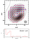 |
Fig. 7 Best fit for the polarization produced by radiation fields from the VLA 5a source (red vectors) and the Band 7 data (blue vectors). The grayscale indicates polarized intensity with same levels of Fig. 1. Vectors are shown for every three pixels. The position angle difference between the our data and the radiation alignment position angles are shown as a histogram in the bottom panel. The histogram bin is 6° –consistent with the largest observational uncertainty in position angle. |
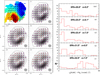 |
Fig. 8 Left panels: synthetic magnetic field lines (red vectors) plotted on top of observed Band 7 Stokes I contours (5–45 mJy beam−1 in steps of 5 mJy beam−1), polarized intensity (grayscale with same intensity levels of Fig. 1), and magnetic fields (blue vectors, which are 90°-rotated with respect to Fig. 1). The red vectors result from our rotating disk modeling assuming different k = Bp ∕Bϕ values. Figure 6 is shown in the upper left panel for reference. Right panels: residuals from each case, with mean δPA = PAdata − PAmodel values and standard deviation σ indicated oneach histogram panel. |
6.3 Interpreting the modeling results
As shown in Figs. 7 and 8, the differences between the observed polarization angles and the model predictions for radiative alignment and magnetic alignment are similar. In both cases the agreement is generally good, but some discrepancies remain between our data and the synthetic maps for some regions of the disk. Although formally the radiative alignment model gives a slightly better fit of the polarization angles than the magnetic alignment model, interpreting our results in terms of the former model presents some difficulties: the observed polarization levels are significantly higher than predicted by Tazaki et al. (2017), and the pattern is more spiral-like than centrosymmetric. In the context of the combined models of self-scattering plus radiative alignment reported in Kataoka et al. (2017), in order to have significant polarization by radiative alignment, one would need grains with sizes of 150 μm. This would imply significant self-scattering polarization in Band 7. However, since we see no signature of self-scattering pattern in our maps, and the observed polarization levels are much higher than the model predictions, it seems unlikely that the polarization arises from radiative alignment. More generally, we do not see the apparent wavelength dependence of the polarization pattern in the different bands, reported in Kataoka et al. (2017) and Stephens et al. (2017).
On the other hand, so long as Larmor precession dominates over radiative precession, the polarization pattern by grains aligned with the magnetic field is not expected to vary with wavelength, as shown by our maps. In addition, the twisting of the magnetic field required to fit our data is in the same sense as the rotation revealed by the molecular line centroid map. The observed discrepancy between the model and our data could be explained in this case by the peculiar nature of the disk: the VLA data indicate a binary system embedded in the disk, which possibly implies the presence of gaps and tiny circumstellar disks around each stellar component. Such an environment is expected to produce substructure in the magnetic field morphology that could distort the large-scale magnetic field components.
Although we cannot rule out alignment with the radiation field, our analysis shows that the observed polarization is consistent with being produced by magnetically aligned grains. The middle and right panels of Fig. 1 show that the polarized radiation is emitted from zones near the outer parts of the disk, where small grains are more abundant. This is an indication that polarization usually traces the external disk layers, which explains the similar polarization patterns in all three bands. In this scenario, the larger millimeter-size grains suggested by our spectral index analysis of the Stokes I emission are located in the disk mid-plane.
7 Conclusions
We have performed multi-frequency ALMA polarization observations toward the young circumbinary disk in BHB07-11. Our observationsreveal extended and ordered polarization in all three bands (3, 6, and 7). Our main conclusions are:
While the total and polarized intensity increases with frequency, the polarization morphology remains the same across the threebands. This gives strong support against polarization mechanisms such as self-scattering and radiation fields, whose predictions are wavelength dependent;
In spite of the asymmetry observed in BHB07-11 and its inclination with respect to the line-of-sight, the polarization structure does not match the self-scattering predictions for lopsided and inclined disks. In addition, the observed polarization levels are at least a factor of four larger than model predictions for scattering polarization in protoplanetary disks (however, similar levels of polarization observed in other objects have been attributed to self-scattering);
Our data do not match models of radiative alignment assuming the flux of VLA 5b or the weighted combined flux of VLA 5a and VLA 5b as sources of radiation, but they match relatively well the predictions if VLA 5a alone is assumed the main source of radiation. However, we cannot explain the discrepancy in the context of this mechanism since the observed spiral-like polarization morphology is inconsistent with the centrosymmetric predictions, and the observed polarization levels are higher than the model predictions.
Our maps are consistent with a model of a rotating disk with a poloidal magnetic field component plus a toroidal component produced by the disk rotation. The synthetic magnetic field lines fit the sense of rotation derived from molecular line maps of the disk. We thus conclude that the polarization in our data is produced by magnetically aligned dust grains.
Acknowledgements
We would like to thank the anonymous referee for a constructive report. This paper makes use of the following ALMA data: ADS/JAO.ALMA#2013.1.00291.S and ADS/JAO.ALMA#2016.1.01186.S. ALMA is a partnership of ESO (representing its member states), NSF (USA) and NINS (Japan), together with NRC (Canada), MOST and ASIAA (Taiwan), and KASI (Republic of Korea), in cooperation with the Republic of Chile. The Joint ALMA Observatory is operated by ESO, AUI/NRAO and NAOJ. JMG is supported by the MINECO (Spain) AYA2014-57369-C3 grant. MP acknowledges funding from the European Unions Horizon 2020 research and innovation program under the Marie Skłodowska-Curie grant agreement No 664931. GAPF acknowledges the partial support from CNPq and FAPEMIG (Brazil). PC acknowledges support of the European Research Council (ERC, project PALs 320620). WV acknowledges support from the ERC through consolidator grant 614264. The data reported in this paper are archived in the ALMA Science Archive.
References
- Alves, F. O., & Franco, G. A. P. 2007, A&A, 470, A597 [NASA ADS] [CrossRef] [EDP Sciences] [Google Scholar]
- Alves, F. O., Girart, J. M., Lai, S., Rao, R., & Zhang, Q. 2011, ApJ, 726, 63 [NASA ADS] [CrossRef] [Google Scholar]
- Alves, F. O., Girart, J. M., Caselli, P., et al. 2017, A&A, 603, L3 [NASA ADS] [CrossRef] [EDP Sciences] [Google Scholar]
- Andersson, B.-G., Lazarian, A., & Vaillancourt, J. E. 2015, ARA&A, 53, 501 [NASA ADS] [CrossRef] [Google Scholar]
- Brooke, T. Y., Huard, T. L., Bourke, T. L., et al. 2007, ApJ, 655, 364 [NASA ADS] [CrossRef] [Google Scholar]
- Cox, E. G., Harris, R. J., Looney, L. W., et al. 2018, ApJ, 855, 92 [NASA ADS] [CrossRef] [Google Scholar]
- Draine, B. T.,& Weingartner, J. C. 1997, ApJ, 480, 633 [NASA ADS] [CrossRef] [Google Scholar]
- Dzib, S. A., Rodríguez, L. F., Araudo, A. T., & Loinard, L. 2013, Rev. Mex. Astron. Astrofis., 49, 345 [NASA ADS] [Google Scholar]
- Frau, P., Galli, D., & Girart, J. M. 2011, A&A, 535, A44 [NASA ADS] [CrossRef] [EDP Sciences] [Google Scholar]
- Girart, J. M., Rao, R., & Marrone, D. P. 2006, Science, 313, 812 [NASA ADS] [CrossRef] [PubMed] [Google Scholar]
- Girart, J. M., Beltrán, M. T., Zhang, Q., Rao, R., & Estalella, R. 2009, Science, 324, 1408 [NASA ADS] [CrossRef] [PubMed] [Google Scholar]
- Girart, J. M., Fernández-López, M., Li, Z.-Y., et al. 2018, ApJ, 856, L27 [CrossRef] [Google Scholar]
- Hull, C. L. H., Plambeck, R. L., Kwon, W., et al. 2014, ApJS, 213, 13 [NASA ADS] [CrossRef] [Google Scholar]
- Hull, C. L. H., Girart, J. M., Tychoniec, Ł., et al. 2017a, ApJ, 847, 92 [NASA ADS] [CrossRef] [Google Scholar]
- Hull, C. L. H., Mocz, P., Burkhart, B., et al. 2017b, ApJ, 842, L9 [NASA ADS] [CrossRef] [Google Scholar]
- Hull, C. L. H., Yang, H., Li, Z.-Y., et al. 2018, ApJ, 860, 82 [NASA ADS] [CrossRef] [Google Scholar]
- Jørgensen, J., Brinch, C., Girart, J. M., et al. 2014, Astrophysics Source Code Library [record ascl:1402.014] [Google Scholar]
- Kataoka, A., Muto, T., Momose, M., et al. 2015, ApJ, 809, 78 [NASA ADS] [CrossRef] [Google Scholar]
- Kataoka, A., Muto, T., Momose, M., Tsukagoshi, T., & Dullemond, C. P. 2016a, ApJ, 820, 54 [NASA ADS] [CrossRef] [Google Scholar]
- Kataoka, A., Tsukagoshi, T., Momose, M., et al. 2016b, ApJ, 831, L12 [NASA ADS] [CrossRef] [Google Scholar]
- Kataoka, A., Tsukagoshi, T., Pohl, A., et al. 2017, ApJ, 844, L5 [NASA ADS] [CrossRef] [Google Scholar]
- Lazarian, A., & Hoang, T. 2007, MNRAS, 378, 910 [Google Scholar]
- Lee, C.-F., Li, Z.-Y., Ching, T.-C., Lai, S.-P., & Yang, H. 2018, ApJ, 854, 56 [NASA ADS] [CrossRef] [Google Scholar]
- Lizano, S., & Galli, D. 2015, in Magnetic Fields in Diffuse Media, eds. A. Lazarian, E. M. de Gouveia Dal Pino, & C. Melioli, Astrophys. Space Sci. Lib., 407, 459 [NASA ADS] [CrossRef] [Google Scholar]
- Natta, A., Testi, L., Calvet, N., et al. 2007, Protostars and Planets V (Arizona: University of Arizona Press), 767 [Google Scholar]
- Padovani, M., Brinch, C., Girart, J. M., et al. 2012, A&A, 543, A16 [NASA ADS] [CrossRef] [EDP Sciences] [Google Scholar]
- Pérez, L. M., Chandler, C. J., Isella, A., et al. 2015, ApJ, 813, 41 [NASA ADS] [CrossRef] [Google Scholar]
- Planck Collaboration Int. XXXV. 2016, A&A, 586, A138 [NASA ADS] [CrossRef] [EDP Sciences] [Google Scholar]
- Rao, R., Girart, J. M., Lai, S.-P., & Marrone, D. P. 2014, ApJ, 780, L6 [NASA ADS] [CrossRef] [Google Scholar]
- Sadavoy, S. I., Myers, P. C., Stephens, I. W., et al. 2018, ApJ, 859, 165 [NASA ADS] [CrossRef] [Google Scholar]
- Shu, F. H., Galli, D., Lizano, S., Glassgold, A. E., & Diamond, P. H. 2007, ApJ, 665, 535 [NASA ADS] [CrossRef] [Google Scholar]
- Stephens, I. W., Yang, H., Li, Z.-Y., et al. 2017, ApJ, 851, 55 [NASA ADS] [CrossRef] [Google Scholar]
- Tazaki, R., Lazarian, A., & Nomura, H. 2017, ApJ, 839, 56 [NASA ADS] [CrossRef] [Google Scholar]
- Yang, H., Li, Z.-Y., Looney, L., & Stephens, I. 2016a, MNRAS, 456, 2794 [NASA ADS] [CrossRef] [Google Scholar]
- Yang, H., Li, Z.-Y., Looney, L. W., et al. 2016b, MNRAS, 460, 4109 [NASA ADS] [CrossRef] [Google Scholar]
- Yang, H., Li, Z.-Y., Looney, L. W., Girart, J. M., & Stephens, I. W. 2017, MNRAS, 472, 373 [NASA ADS] [CrossRef] [Google Scholar]
- Zhang, Q., Qiu, K., Girart, J. M., et al. 2014, ApJ, 792, 116 [NASA ADS] [CrossRef] [Google Scholar]
All Figures
|
Fig. 1 StokesI (left panel), polarized intensity (middle panel), and polarization fraction (right panel) of our Band 3 (upper panels), Band 6 (middle panels), and Band 7 (lower panels) ALMA data. The contours indicate the intensity levels of the Stokes I emission in each band, being 30, 60, 90, 120, 150, and 180 times the rms for bands of 3 and 6 (rmsBand 3 ~ 0.012 mJy beam−1 and rmsBand 6 ~ 0.15 mJy beam−1), and 30, 60, 90, 120 times 0.52 mJy beam−1, the rms for Band 7. The synthesized beams are 0.22′′ × 0.17′′ (position angle = −61.46°) for Band 3, 0.26′′ × 0.15′′ (position angle = −85.65°) for Band 6 and 0.21′′ × 0.18′′ (position angle = −72.79°) for Band 7. The vector map indicates the orientation of the polarization whose length is proportional to the polarization fraction. The vectors are sampled as one vector every two pixels. The two star symbols in the middle-lower panel indicate the position of the two continuum peaks detected in the 34 GHz VLA data, VLA 5a for the northern peak and VLA 5b for the southern one (see also Fig. 2). |
| In the text | |
|
Fig. 2 Intensity contours of the 34 GHz VLA emission plotted on top of the Band 7 Stokes I image of BHB07-11. The contours correspond to intensity levels of 3, 5, 7, …, 15, 17 × the noise level of the VLA map, 12 μJy beam−1. The VLA synthesized beam of 0.10′′ × 0.04′′ is shown in the lower left corner. |
| In the text | |
|
Fig. 3 Distribution of polarization angles for each band using a bin of 10°. |
| In the text | |
|
Fig. 4 Distribution of the polarized intensity as a function of total intensity. The mean polarization fraction over the regions shown in the right panels of Fig. 1 are indicated in each panel as straight lines. The rms (error bars) for the polarized intensity and total intensity are mentioned in Sect. 2.1. |
| In the text | |
|
Fig. 5 Spectral index map obtained from the Stokes I emission between Bands 3 and 7. The Stokes I maps were smoothed to a common circular beam of 0.25′′ prior to spectral index computation. The contours show the Stokes I Band 7 flux as in Fig. 1. |
| In the text | |
|
Fig. 6 Polarization vectors rotated by 90° showing the plane-of-sky magnetic field configuration at Band 7. Contours show the same Stokes I intensity levels as in Fig. 1. The background image is a moment 1 map of the H2 CO (32,1 − 22,0) emission in BHB07-11. The moment map is produced from a 3σ cut (σ ~ 5.3 mJy beam−1) in the molecular emission. The synthesized beam of the H2CO map is 0.27′′ × 0.21′′. The stars symbols have the same meaning as in Fig. 1. |
| In the text | |
|
Fig. 7 Best fit for the polarization produced by radiation fields from the VLA 5a source (red vectors) and the Band 7 data (blue vectors). The grayscale indicates polarized intensity with same levels of Fig. 1. Vectors are shown for every three pixels. The position angle difference between the our data and the radiation alignment position angles are shown as a histogram in the bottom panel. The histogram bin is 6° –consistent with the largest observational uncertainty in position angle. |
| In the text | |
|
Fig. 8 Left panels: synthetic magnetic field lines (red vectors) plotted on top of observed Band 7 Stokes I contours (5–45 mJy beam−1 in steps of 5 mJy beam−1), polarized intensity (grayscale with same intensity levels of Fig. 1), and magnetic fields (blue vectors, which are 90°-rotated with respect to Fig. 1). The red vectors result from our rotating disk modeling assuming different k = Bp ∕Bϕ values. Figure 6 is shown in the upper left panel for reference. Right panels: residuals from each case, with mean δPA = PAdata − PAmodel values and standard deviation σ indicated oneach histogram panel. |
| In the text | |
Current usage metrics show cumulative count of Article Views (full-text article views including HTML views, PDF and ePub downloads, according to the available data) and Abstracts Views on Vision4Press platform.
Data correspond to usage on the plateform after 2015. The current usage metrics is available 48-96 hours after online publication and is updated daily on week days.
Initial download of the metrics may take a while.