| Issue |
A&A
Volume 616, August 2018
|
|
|---|---|---|
| Article Number | A104 | |
| Number of page(s) | 18 | |
| Section | Stellar structure and evolution | |
| DOI | https://doi.org/10.1051/0004-6361/201832831 | |
| Published online | 28 August 2018 | |
Non-linear seismic scaling relations
1
Institute for Astrophysics, University of Vienna,
Türkenschanzstrasse 17,
1180
Vienna,
Austria
e-mail: thomas.kallinger@univie.ac.at
2
Instituto de Astrofísica de Canarias,
38200
La Laguna,
Tenerife,
Spain
3
Departamento de Astrofísica, Universidad de La Laguna,
38206
La Laguna,
Tenerife,
Spain
4
School of Physics, University of New South Wales,
Sydney
NSW 2052,
Australia
5
Sydney Institute for Astronomy (SIfA), School of Physics, University of Sydney,
Sydney
NSW 2006,
Australia
6
Stellar Astrophysics Centre, Department of Physics and Astronomy, Aarhus University,
Ny Munkegade 120,
8000
Aarhus C,
Denmark
7
IRFU, CEA, Université Paris-Saclay,
91191
Gif-sur-Yvette,
France
8
Université Paris Diderot, AIM, Sorbonne Paris Cité, CEA, CNRS,
91191
Gif-sur-Yvette,
France
Received:
14
February
2018
Accepted:
15
May
2018
Context. In recent years the global seismic scaling relations for the frequency of maximum power, νmax ∝ g / √Teff, and for the large frequency separation, Δν ∝ √ρ¯, have drawn attention in various fields of astrophysics. This is because these relations can be used to estimate parameters, such as the mass and radius of stars that show solar-like oscillations. With the exquisite photometry of Kepler, the uncertainties in the seismic observables are small enough to estimate masses and radii with a precision of only a few per cent. Even though this seems to work quite well for main-sequence stars, there is empirical evidence, mainly from studies of eclipsing binary systems, that the seismic scaling relations systematically overestimate the mass and radius of red giants by about 15% and 5%, respectively. Various model-based corrections of the Δν-scaling reduce the problem but do not solve it.
Aims. Our goal is to define revised seismic scaling relations that account for the known systematic mass and radius discrepancies in a completely model-independent way.
Methods. We use probabilistic methods to analyse the seismic data and to derive non-linear scaling relations based on a sample of six red giant branch (RGB) stars that are members of eclipsing binary systems and about 60 red giants on the RGB as well as in the core-helium burning red clump (RC) in the two open clusters NGC 6791 and NGC 6819.
Results. We re-examine the global oscillation parameters of the giants in the binary systems in order to determine their seismic fundamental parameters and we find them to agree with the dynamic parameters from the literature if we adopt non-linear scalings. We note that a curvature and glitch corrected Δνcor should be preferred over a local or average value of Δν. We then compare the observed seismic parameters of the cluster giants to those scaled from independent measurements and find the same non-linear behaviour as for the eclipsing binaries. Our final proposed scaling relations are based on both samples and cover a broad range of evolutionary stages from RGB to RC stars: g / √Teff = (νmax / νmax,⊙)1.0075±0.0021 and √ρ¯ = (Δνcor / Δνcor,⊙)[η − (0.0085 ± 0.0025) log2(Δνcor / Δνcor,⊙)]−1, where g, Teff, and ρ¯ are in solar units, νmax,⊙ = 3140 ± 5 μHz and Δνcor,⊙ = 135.08 ± 0.02 μHz, and η is equal to one in the case of RGB stars and 1.04 ± 0.01 for RC stars.
Conclusions. A direct consequence of these new scaling relations is that the average mass of stars on the ascending giant branch reduces to 1.10 ± 0.03 M⊙ in NGC 6791 and 1.45 ± 0.06 M⊙ in NGC 6819, allowing us to revise the clusters’ distance modulus to 13.11 ± 0.03 and 11.91 ± 0.03 mag, respectively. We also find strong evidence that both clusters are significantly older than concluded from previous seismic investigations.
Key words: stars: fundamental parameters / stars: oscillations / stars: late-type / stars: interiors / open clusters and associations: individual: NGC 6819 / open clusters and associations: individual: NGC 6791
© ESO 2018
1 Introduction
Mass and radius are amongst the most fundamental stellar parameters. Knowing them is essential to characterise a star, but also a prerequisite to characterise a planet orbiting that star. A frequently used method to determine stellar mass and radius is by comparing some observed properties, such as effective temperature and surface gravity, to those of stellar evolutionary tracks and deriving a set of best-fit model parameters (mass, radius, age, etc.). This method is, however, quite uncertain not only because of the often large observational uncertainties but also because of large and frequently ignored systematic uncertainties in the models (e.g. Stancliffe et al. 2016). A direct measurement of stellar mass is possible through radial velocity measurements for stars with well-known inclinations such as eclipsing, double-lined spectroscopic binaries (SB2), or through precise astrometry or interferometry of visually resolved wide binaries. In such cases, the mass can be measured with high accuracy and precision (<3%), but there are only a few such systems known.
Another method to infer stellar fundamental parameters is by means of asteroseismology (e.g. see the monograph by Aerts et al. 2010), in particular for cool stars with a convective surface layer (hence stars ranging from cool F to M on the main sequence and high up the giant branch). They are believed to show so-called solar-like oscillations, which are intrinsically damped and stochastically excited by the turbulence in the near-surface convection. Their oscillation spectrum presents a nearly regular frequency pattern of modes, which carry information about the internal structure of the star.
The simplest analysis of solar-like oscillations is based on the “global” properties of the oscillations, which are the large frequency separation, Δν, between consecutive modes of the same spherical degree, l, and the frequency of the maximum oscillation power, νmax, which we will call peak frequency for short.
The large frequency separation is related to the inverse sound travel time across the stellar diameter, essentially scaling with the mean stellar density  (e.g. Brown & Gilliland 1994) as,
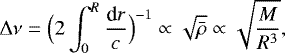 (1)
(1)
where c is the sound speed and M and R are the stellar mass and radius, respectively. The peak frequency, however, is related to the acoustic cut-off frequency νac in the stellar atmosphere (e.g. Brown et al. 1991; Kjeldsen & Bedding 1995), which in turn scales with the stellar surface gravity g and effective temperature Teff as,
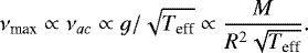 (2)
(2)
From this pair of scaling relations – commonly called global asteroseismic scalings – and a measurement for the effective temperature, one can estimate a star’s surface gravity and mean density and subsequently its mass and radius by scaling νmax and Δν to those of the Sun (e.g. Kallinger et al. 2010a,b).
One might expect that the solar reference values are simple to measure but in practise a number of values can be found in the literature (e.g. Kjeldsen & Bedding 1995; Huber et al. 2011; Mosser et al. 2013) that differ by more than the individual uncertainties. For the large separation this is largely because Δν is in fact a function of frequency (see e.g. Broomhall et al. 2009) and therefore depends on the frequency range for which it is measured. To measure the peak frequency requires a separation of the oscillation signal from the underlying granulation background and unwarranted assumptions about the latter can bias the measurement (Kallinger et al. 2014). Using the seismic scaling relations therefore requires well-defined and consistently measured global oscillation parameters.
In practice, measurements of the asteroseismic global parameters have been extensively used to estimate masses and radii for stars with solar-like oscillations detected in CoRoT (Baglin et al. 2006) and Kepler (Borucki et al. 2010) data. For more details we refer to the reviews by Chaplin & Miglio (2013) and Garcia & Stello (2018). Given the importance of the seismic scalings, several studies have tried to test their validity, but mostly focused on the  scaling because so far there is no secure theoretical basis for predicting νmax (e.g. Belkacem et al. 2011). However, Viani et al. (2017) recently reported on a mean molecular weight and adiabatic index term in the νac -scaling of their stellar model.
The available studies that examine the Δν -scaling follow one of two approaches: those testing the scalings with independently determined radii (e.g., from interferometry) and those confronting the scaling with model predictions. The observational approach shows generally good agreement (within ~4% and 16% for main-sequence stars and red giants, respectively (see e.g. Huber et al. 2012; Baines et al. 2014) but are limited by the uncertainties of the non-seismic benchmarks observations. This is because, currently, seismic targets from CoRoT or Kepler are typically quite faint. The theoretical approach (e.g. White et al. 2011; Guggenberger et al. 2016; Sharma et al. 2016), on the other hand, is in principle more accurate but has to deal with systematic effects in the models (such as the so-called “surface effect”; e.g. Gruberbauer et al. 2013, Li et al. 2018), which hamper a comparison between scaled Δν and those determined from the model frequencies.
To validate seismic masses is even less practicable. In conclusion, even though the exquisite photometry of CoRoT and Kepler allows us to estimate seismic masses and radii to a precision of a few per cent, the underlying scaling relations cannot be confirmed to better than about 4% and 16% for main-sequence and red giant stars, respectively.
A promising way to improve the situation is given by eclipsing double-lined spectroscopic binary (eSB2) systems hosting at least one star with detectable solar-like oscillations. Complementary photometric observations of the eclipses and radial velocity measurements of the orbital motions allow us to accurately constrain the orbital inclination and therefore the dynamic masses and radii of both components, even for quite faint stars. The first such reported system, KIC 8410637, was detected by Hekker et al. (2010), and Frandsen et al. (2013) found good agreement between the seismic and dynamic estimate of log g for the oscillating red giant component. However, Huber (2014) noted that the seismic and dynamic radius and mass deviate by about 9% (2.7σ) and 17% (1.9σ), respectively, indicating that the seismic scaling relations need some revision.
This was confirmed by a recent study by Gaulme et al. (2016), who investigated a sample of ten eSB2 systems observed by Kepler with supplementary radial velocity observations, from which they could detect solar-like oscillations and measure dynamic masses and radii. They found that whereas the agreement between seismic and dynamic surface gravities is acceptable, the seismic scalings systematically overestimate the radii and masses by about 5% and 15%, respectively, for various stages of red giant evolution. An immediate consequence of this is that an age estimate based on the seismic mass (via grid modelling, e.g. Stello et al. 2009; Basu et al. 2010; Kallinger et al. 2010a; Quirion et al. 2010; Gai et al. 2011; Creevey et al. 2013; Hekker et al. 2013; Miglio et al. 2013; Serenelli et al. 2013) substantially underestimates the actual stellar age, which would be a serious issue for applications such as galactic archaeology.
In this paper, we re-examine the seismic analysis of the key set of stars in the Gaulme et al. (2016) sample and use the dynamic mass and radius measurements by Gaulme et al. (2016), Brogaard et al. (2018), and Themeßl et al. (2018) to formulate new non-linear1 scaling relations for νmax and Δν. We then compare the observed seismic parameters of more than 60 red giants in the two open clusters NGC 6791 and NGC 6819 to those scaled from independent measurements and find them to show the same non-linear behaviour as the eclipsing binaries. We use this to refine the scaling coefficients and to extend the scalings to a broader range of evolutionary stages on the giant branch, including red clump stars. Finally, we discuss the resulting decrease of the average mass of stars on the red giant branch (RGB) of the two clusters and its consequences for the age determination.
2 Gaulme’s sample of oscillating red giants in eclipsing binaries
Gaulme et al. (2016; hereafter G16) reported on a four-year radial velocity (RV) survey for a sample of eclipsing binary systems discovered by Kepler. By combining the RV measurements and the photometric Kepler observations of the eclipses, they determined the dynamical mass and radius for 14 double-lined spectroscopic binaries. Ten of these systems include a red giant that shows clear solar-like oscillations in the Kepler photometry, for which they determined global seismic parameters. This allowed G16 to straightforwardly test the seismic scaling relations with high precision and accuracy, for the first time. We go beyond that and use their key set of stars to derive new seismic scalings for red giants. Since not all systems are suitable for such an analysis, we selected six out of the original ten binaries. The remaining four systems have either observations of insufficient accuracy or ambiguous evolutionary phases of the red giant components (see Sect. 3). Our sample of stars is listed in Table 1.
Stellar parameters for the six known eSB2 in the Kepler sample from dynamical modelling and asteroseismic scaling.
2.1 Defining our sample
Two stars ofour sample were also analysed by Themeßl et al. (2018; hereafter T18), who reanalysed the spectroscopy obtained by Frandsen et al. (2013) and Beck et al. (2014). In the G16 analysis, the dynamic mass and radius of KIC 8410637 are based on the original analysis of Frandsen et al. (2013) using the eclipses covered by Kepler between Q1 and Q10. With the full Kepler data available, T18 refined the dynamic parameters. For KIC 9540226, G16 had to fix the system inclination to 90° to help the fit to converge. T18 solved this problem and found a slightly lower inclination resulting in somewhat different but more reliable dynamic parameters.
Two more stars were also investigated by Brogaard et al. (2018; hereafter B18), who used additional spectroscopic observationsto refine the dynamic solutions for KIC 7037405 and KIC 9970396. KIC 9540226 was analysed by all three groups and while the mass estimates are in good agreement, the dynamic radius differs by about 1.6σ between T18 and B18. We adopt the solution from T18 because they provide a more accurate mass but note that using the values from B18 does marginally affect our subsequent analysis. To summarise, for our sample of six stars, we adopt the dynamic parameters for two stars each from the original G16 analysis, from T18, and from B18, respectively. This diversity in source should make our analysis largely independent of any specific instrument (for the spectroscopy) and analysis method. All dynamic parameters are listed in Table 1.
2.2 Effective temperature scale
A possible source for the discrepancy between the seismic and dynamic masses and radii is the temperature scale applied to the seismic scalings. Beck et al. (2018a) pointed out that the stars reported in the sample of G16 are systematically hotter by a few 10 K than stars in the sample of Beck et al. (2014). They also concluded that the difference is not big enough to reconcile the mass discrepancy between seismically and dynamically inferred masses. To cover the entire reported offsets one would, however, need to change Teff by about 10% or 500 K for a typical red giant with an effective temperature of 4800 K, which seems not very plausible. In fact, the effective temperatures of our sample stars from various sources are generally in good agreement (see Fig. 1). We find a maximum difference of 127 K for the reported Teff values, which can certainly not account for the discrepancy between the seismic and dynamic masses and radii. To be consistent with other Kepler red giants we use the effective temperatures from the APOKASC catalogue (DR13; Pinsonneault et al. 2014) representing an asteroseismic and spectroscopic joint survey of stars in the Kepler field. For KIC 5786154 there is no Teff estimate available in the APOKASC catalogue, which is why we use the original value from G16 for this star. A detailed comparison with other Teff sources may be found in G16, showing a similar picture.
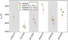 |
Fig. 1 Comparison of Teff from various sources for our sample of red giants in eSB2 systems. |
3 Re-examining the global seismic parameters and their associated fundamental parameters
All photometric time series used in this analysis have been obtained with the NASA Kepler space telescope spanning from quarter 2 to 17 with a total length of about 1420 d. The Kepler raw SAP-FLUX measurements2 were smoothed with a triangular filter to suppress intrinsic and instrumental long-term trends with timescales longer than about 10 d. Even though Kepler is supposed to observe continuously, there are several instances where scientific data acquisition is affected, producing quasi-regular gaps (García et al. 2014). Gaps that are shorter than about 3/νmax are filled by linear interpolation improving the duty cycle from about 93% to about 95%. This is sufficient to correct for most of the objectionable regularities in the spectral window function (Kallinger et al. 2014).
In a first step, we re-examined the seismic analysis for the G16 sample following the methods described in Kallinger et al. (2010a, 2012, 2014) and found sufficiently accurate results for seven of the original ten stars. For KIC 7377422 the oscillation modes are too weak to make any firm conclusions. For KIC 10001167 and KIC 4663623 the seismic and dynamic uncertainties, respectively, are too large to include the stars in the further analysis. We do, however, note that excluding the latter two stars does only marginally change the main result of our analysis but improves the final uncertainties.
3.1 The peak frequency νmax
To determine the peak frequency we adopt the approach of Kallinger et al. (2014) and fit a global model to the observed power density spectra, where we restrict the spectra to between 0.1νmax and the Nyquistfrequency. The model consists of a flat noise component, two super-Lorentzian functions with an exponent fixed to four, and a Gaussian with the central frequency representing νmax. For the fit we use the Bayesian nested sampling algorithm MULTINEST (Feroz et al. 2009, 2013), which delivers posterior probability distributions for the parameters estimation and a so-called global model evidence. The latter is a statistical measure that allows us to reliably rate whether a given model represents the observations better than some other model.
The resulting peak frequencies agree with those reported by G16 on average to within 2σ. For five of the six stars, however, our νmax is larger than those from G16 (by on average 1.6%). The reason for this is likely due to a different treatment of the background signal. Kallinger et al. (2014) systematically compared various background models and found systematic differences in νmax depending on the specific treatment of the granulation signal. Even though G16 used the same model for the granulation signal as we do, they added a coloured-noise component (as suggested by Kallinger et al. 2014). To further investigate this we repeated the fits now following the exact approach of G16 (Gaulme, priv. comm.) and compared the resulting model evidence delivered by MULTINEST. Interestingly, the additional coloured-noise component is statistically justified only for KIC 9540226. For the other five stars it represents an overfitting of the data presumably distorting the granulation model and causing a small but systematic underestimation of νmax. We therefore prefer our values of νmax for the subsequent analysis (see Table 1).
3.2 The central large separation Δνc
For the large frequency spacing, G16 follow the approach of Mosser et al. (2011) to compute an average Δν from the universal pattern, which is then converted into an asymptotic Δν using the semi-empirical relation of Mosser et al. (2013) (see Sect. 3.4). They thereby use a fixed conversion factor (1 + ζ), with ζ = 0.038. Such a fixed conversion does, however, not account for the observed variety of the mode curvature of up to some 10% (see Fig. 6 in Mosser et al. 2013), which add an additional uncertainty of 1%–2% to the random error of typically 0.1% in Δν as given by G16.
We think that the use of a scaled asymptotic Δν in a star-by-star analysis, rather than in an ensemble sense, does in fact impair rather than improve the subsequent analysis if the departure from regular frequency spacing in the form of “curvature” and “glitch” properties are not measured for each star (see Sect. 3.4). This is why we prefer to use an observed value of Δν. More specifically, we start our analysis with the average frequency spacing of the three central radial orders Δνc, which is determined by fitting a sequence of eight Lorentzian profiles to the power density spectra. The model covers three consecutive orders of l = 0 and 2 modes and the intermediate l = 1 modes, whose frequencies are parameterised by the frequency of the central radial mode and a large and small frequency separation. For the fit we use again MULTINEST and refer to Kallinger et al. (2010a, 2012) for more details about the automated approach. The seismic parameters and their uncertainties are listed in Table 1.
3.3 Evolutionary stage
An often used method to evaluate the evolutionary state of a red giant is by means of the period spacing of its mixed dipole modes (e.g. Bedding et al. 2011; Mosser et al. 2014). For many of the stars in our sample this is, however, not possible because either the frequency resolution or the signal-to-noise ratio (S/N) of the modes is not sufficient. We therefore determine the evolutionarystage from the phase shift of the central radial mode (Kallinger et al. 2012; Christensen-Dalsgaard et al. 2014) and find that all but one star in the original G16 sample are ascending RGB stars. Only for KIC 9246715 are we unable to clearly determine if it is a H-shell burning star or a core-He burning star that has not experienced a helium flash on the tip of the giant branch (also called a secondary clump star). Gaulme et al. (2014) and later on Rawls et al. (2016) classified this star as a secondary clump star, which is why we remove it from our sample. We further note that we find an independent classification only for KIC 9970396, which is identified as an RGB star by Elsworth et al. (2017).
3.4 The asymptotic large separation Δνas
The frequencies of low-degree and high-order acoustic modes approximately follow an asymptotic relation (Tassoul 1980; Gough 1986), which reduces in its simplest form for radial modes (l = 0) to
 (3)
(3)
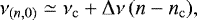
when linked to the frequency of the central radial mode of the oscillation power excess (meaning the radial mode closest to νmax), where n is a mode’s radial order and the subscript c denotes values for the central radial mode. This form can clearly not account for an accurate description of the observed radial mode pattern in red giants. They show a noticeable curvature in the échelle diagram (Fig. 2) at all evolutionary stages (e.g. Kallinger et al. 2012) so that higher order terms in the asymptotic expansion need to be considered.
Following Mosser et al. (2011), the second-order development of the asymptotic theory can be described with a curvature term α:
![\begin{equation*}\nu_{(n,0)} \simeq \nu_{\mathrm c} + {{\mathrm \Delta}}\nu_{\mathrm cor} \, \Big[n-n_{\mathrm c} + \frac{\alpha}{2}(n-n_{\mathrm c})^2\Big], \end{equation*}](/articles/aa/full_html/2018/08/aa32831-18/aa32831-18-eq11.png) (4)
(4)
where Δνcor represents the corrected frequency difference between radial modes at the central radial mode. Strictly speaking, Eq. (1) is, however, defined for the large separation at infinitely high frequencies and not at νmax, so that Δνcor needs to be linked to the asymptotic large separation Δνas (Mosser et al. 2013) as
![\begin{equation*}{{\mathrm \Delta}}\nu_{\mathrm as} = {{\mathrm \Delta}}\nu_{\mathrm cor}\, \Big[1 + \frac{\alpha \,n_{\mathrm c}}{2} \Big]. \end{equation*}](/articles/aa/full_html/2018/08/aa32831-18/aa32831-18-eq12.png) (5)
(5)
The curvature term is clearly responsible for the difference between the observed and asymptotic values of the large separation and correcting for it should improve the  scaling.
Mosser et al. (2013) measured the curvature terms for a few red giants to determine a relation α(Δν), which intends to convert an observed value of Δν into a physically grounded asymptotic value without the need for an in-depth analysis of the mode pattern. The scaling is, however, only based on a small number of stars and does not account for the relatively large scatter of α independent of Δν. Hence, using α(Δν) adds significant uncertainties to Δνas. This might be acceptable in a statistical sense for a large sample of stars but certainly not for the detailed analysis of our sample of eclipsing double-lines spectroscopic binary (eSB2) stars. We therefore intend to measure the curvature term individually. To do so, another effect needs to be taken into account.
Vrard et al. (2015) have shown that the observed deviations from Eq. (4) can be characterised in terms of the location of the second ionisation zone of helium (e.g. Houdek & Gough 2007). They use the second-order expansion to correct the observed frequencies for curvature and fit a harmonic term to the residuals. Here we are more interested in the curvature term and therefore expand the asymptotic relation to
![\begin{equation*}\nu_{(n)} = \nu_{\mathrm c} + {{\mathrm \Delta}}\nu_{\mathrm cor} \, \Big[n - n_{\mathrm c} + \frac{\alpha}{2}(n-n_{\mathrm c})^2 + A\sin\Big(2\pi\,\Big(\frac{n-n_{\mathrm c}}{G}+\phi_{\mathrm c}\Big)\Big) \Big], \end{equation*}](/articles/aa/full_html/2018/08/aa32831-18/aa32831-18-eq14.png) (6)
(6)
where the harmonic term accounts for the periodic frequency modulation caused by the second helium ionisation zone, often called the glitch signal. The parameter A, G, and ϕc are the glitch term’s amplitude, period, and phase, respectively, at the central radial mode. We note here that it is not necessary to specifically consider the crosstalk between parameters, like α and G. Any possible crosstalk will be reflected in the posterior probability distributions delivered by MULTINEST, from which we determine the most likely parameters and their uncertainties. We further note that α from Eqs. (4) and (6) turn out to be practically identical.
To determine the curvature and the glitch parameters we first need the frequencies of the radial modes. Our method to determine Δνc (Sect. 3.2) also provides an estimate of νc (see Kallinger et al. 2010a, 2012, for more details), which we use to predict the initial positions of the radial modes. To extract their frequencies, we fit Lorentzian profiles to the power density spectrum again using MULTINEST and consider a mode as statistically significant ifthe model evidence provided by MULTINEST is at least ten times larger than for a fit with a straight line (meaning only noise)3. We then fit Eq. (6) to the extracted mode frequencies to determine the curvature and glitch parameters. We again fit various models (straight line, Eqs. (4), and (6)) to determine the significance of the result. The resulting Δνcor and Δνa s values are listed in Table 1. As an example, Fig. 2 shows the power density spectrum and échelle diagram of the radial modes for KIC 9970396 along with the best fit. More details about the mode fitting and the curvature and glitch analysis are the subject of a separate paper (Kallinger et al., in prep.).
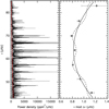 |
Fig. 2 Left: original (grey line) and smoothed (black line) power density spectrum of KIC 9970396. The red line indicates the granulation background. Right: échelle diagram of the significant radial modes. The solid and dashed lines correspond to our asymptotic fit (Eq. (6)) and the curvature term of the fit, respectively. |
3.5 Solar-calibrated seismic fundamental parameters from νmax and Δνc
By comparing Δν and νmax to the respective solar reference values, we can now easily determine the mean stellar density and surface gravity, and subsequently the mass and radius, from Eqs. (1) and (2). To ensure a consistent internal calibration, the solar low-degree oscillation spectrum needs to be analysed with the same tools as used for the stellar power density spectra. We refer to Δνc,⊙ = 134.88 ± 0.04 μHz (Kallinger et al. 2010a) and νmax ,⊙ = 3140 ± 4 μHz (Kallinger et al. 2014) as solar reference values, which are both determined from one-year time series from the green channel of the SOHO/VIRGO data (Frohlich et al. 1997) during solar minimum 23. The resulting seismic masses and radii of our set of stars have internal uncertainties of about 3.8% and 2.0%, respectively. A comparison between the dynamic and solar-calibrated seismic parameters is shown in Fig. 3 (grey symbols). We find rather small deviations between the seismic and dynamic surface gravities (0.014 ± 0.008) and mean densities (− 2.5 ± 1.8%). They do, however, translate into significant deviations when converted into R (6.4 ± 2.6%) and M (17 ± 7%), which is fully consistent with the result of G16 (see Table 2).
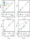 |
Fig. 3 Seismic vs. dynamic parameters for our sample of seven eSB2 binaries. The four main panels show the direct comparison for each of the four parameters log g, |


Average systematic deviation, χ, and its rms scatter, between dynamic and seismic parameters for different input Δν and reference values.
3.6 Model-calibrated seismic fundamental parameters from νmax and Δνc
White et al. (2011) and only recently Guggenberger et al. (2016) and Sharma et al. (2016) suggested that the observed Δν could be corrected with an empirical function, which they deduce from stellar models. They found that the computed radial eigenfrequencies of stellar models have a large separation that does not exactly follow the  scaling. The deviations are on the order of up to a few percent and depend on the effective temperature and chemical composition of the models. We apply their corrections to Δνc and compute the resulting mean density (Table 2), which in fact sufficiently aligns the
  scaling. However, if we compute the stellar radius and mass from this, we still find systematic deviations of 2%–4% and 8%–12%, respectively. This is because also the νmax − g scaling shows a systematic deviation.
Now, anobvious problem in such model-dependent approaches is that the model frequencies suffer from systematic errors, such as the so-called surface effect (e.g. Kjeldsen et al. 2008), which is an offset between observed and computed oscillation frequencies. For the Sun, the offset is known to increase with frequency and hence affects the large separation with Δν, being about 1% larger in the models than observed (e.g. Houdek et al. 2017). For more evolved stars, Sonoi et al. (2015), Ball & Gizon (2017), and only recently Li et al. (2018) suggested surface-effect corrections, from which we conclude that the model Δν is affected on the order of 1%–2%. Furthermore, Gruberbauer et al. (2013) found evidence that the surface effect significantly varies across the Hertzsprung–Russell (HR) diagram and can even be “anti-solar”. We therefore think that the Δν corrections that arise from stellar models are rather connected to the surface effect in stellar models but do not in their current form reliably reflect the  scaling of real stars.
3.7 Solar-calibrated seismic fundamental parameters from νmax and Δνas
To determine a new set of seismic fundamental parameters, which are now based on νmax and Δνas, first requires an asymptotic value for the solar large separation. Applying the same procedure as in Sect. 3.4 to solar data gives 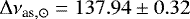 μHz, which agrees well with the value derived by Mosser et al. (2013, see their Table 1).
The seismic surface gravities stay unchanged but while the Δνc-based mean stellar densities underestimate the dynamic values on average by about 2.5%, the new Δνas-based densities overestimate the dynamic ones by almost 7% (see Table 2). Since  and
and  , the resulting seismic masses and radii from Δνas are smaller than the Δνc-based values and do in fact agree well with the dynamic estimates with only small systematic differences (see Table 2).
Mosser et al. (2013) argued that the asymptotic large separation is a physically more meaningful representation of the mean stellar density than an observed value of Δν and should therefore result in more realistic masses and radii (see also Belkacem et al. 2013). We agree on the first part of the argument and clearly the Δνas-based masses and radii agree better with the dynamic measurements than the Δνc-based results do (see Table 2). However, this apparent agreement is because the systematic deviations in g and  , which represent the misaligned scaling between the seismic measurements and the physical properties of the star, almost cancel out when M and R are computed. The improvements in M and R are therefore largely due to the mathematical characteristic of the scalings. In fact the
  scaling is even more misaligned than the
  but in the opposite direction. We think the reason for this is due to the solar reference values and that the scalings are not strictly homologous.
4 The non-linearity of the scaling relations
Using the Sun as a reference for red giants implicitly assumes that the interior structure of a red giant scales linearly with the solar structure, meaning that the two are homologous. This is clearly not the case and it is therefore not surprising to find inherent systematic inaccuracies in the seismic-based fundamental parameters of red giants, such as mass and radius. A better approach would be to scale the seismic observables relative to those of one or more stars of similar interior structure. Our sample of eSB2 stars allows this for the first time with sufficient accuracy.
For thepeak frequency we follow Eq. (2) and compare the measured νmax to  (all in solar units) and find the resulting ratio to differ significantly from the solar reference, with an average value of νmax,RGB = 3245 ± 50 μHz (see Fig. 4, top panel). This indicates that the solar peak frequency is not well-suited as a reference for red giants. Strictly speaking, this might only be valid for RGB stars with a νmax in the range covered by the eSB2 stars (about 20 to 80 μHz). For a more general approach, we fit the dynamic parameters with
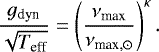 (7)
(7)
For the fit we use again MULTINEST, which like any other fitting algorithm can only consider uncertainties in the dependent variable, in our case  ). To also account for the uncertainties of the independent variable (νmax ∕νmax,⊙) we first add normal distributed uncertainties to the dependent variable with σ being equal to the actual uncertainties of the individual measurements, and then redo the fit, adding up a probability density distribution for the exponent, κ. We iterate this procedure until the fitting parameter converges to a value that stays within 1% of the corresponding uncertainty. The resulting accumulated probability density distribution is then fit by a Gaussian in order to determine the most likely parameter and its uncertainty. We find κ = 1.0080 ± 0.0024, which is more than 3σ different from unity, representing linear scaling. Even though this is only based on six stars, we note that the Bayesian model evidence for the non-linear νmax-scaling is significantly better than for the linear scaling with a fixed νmax,RGB. This makes also more sense from a physical point of view as Eq. (7) does smoothly connect the giant branch to the solar regime, where (νmax∕νmax,⊙) approaches one.
For the large separation we find a similar situation (see Fig. 4 for Δνc and Δνcor). As for the peak frequency, an average reference value Δνc,RGB = 133.1 ± 1.3 μHz, determined from our six eSB2 stars, improves the alignment of the linear  scaling but is again statistically insignificant compared to a power law of the form
  . However, we find that the function
![\begin{equation*}{{\mathrm \Delta}}\nu = {{\mathrm \Delta}}\nu_{\mathrm ref} \cdot \sqrt{ \bar\rho_{\mathrm dyn}} = {{\mathrm \Delta}}\nu_{\odot}\, \left [1- \gamma \log^2{({{\mathrm \Delta}}\nu/{{\mathrm \Delta}}\nu_{\odot})} \right ] \cdot \sqrt{ \bar\rho_{\mathrm dyn}}, \end{equation*}](/articles/aa/full_html/2018/08/aa32831-18/aa32831-18-eq29.png) (8)
(8)
gives even better statistical evidence, with an odds ratio of about 14:1. The MULTINEST fit gives γ = 0.0043 ± 0.0025 and 0.0085 ± 0.0025 for Δνc and Δνcor, respectively, again considering the uncertainties of all parameters. As for νmax (Eq. (7)), the newly established Δνref is smoothly linked to the solar regime and will likely also give plausible results for stars with Δν outside the range of our eclipsing benchmark stars of about 3–7 μHz. While anchoring to the solar case practically ensures reasonable results for stars with higher Δν, for lower Δν an extrapolation is involved, which makes the results more questionable. In Sect. 5, however, we verify Eq. (8) for stars with Δν down to about 0.9 μHz.
For the asymptotic large separation we do not find a gradually decreasing reference value. In fact, the scatter is much larger than for Δνc and Δνcor and we can only establish an average reference value of Δνas,RGB = 142.2 ± 1.6 μHz.
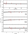 |
Fig. 4 Reference values for νmax (top panel) and Δν (bottom three panels) that result from the ratio of the seismic and dynamic parameters (in solar units). The dashed lines indicate the solar reference value. The full black lines show the new reference values and the grey-shaded range shows their uncertainties. |
4.1 Re-determined seismic fundamental parameters
Above we have determined RGB-calibrated reference values for the classical linear scaling relations (Eqs. (1) and (2)) and established new non-linear scaling relations (Eqs. (7) and (8)). We now apply these scalings to re-detemine the seismic fundamental parameters of our sample stars.
In a first step, we use the RGB-calibrated average reference values νm ax,RGB and Δνc,RGB, Δνcor,RGB, and Δνas,RGB and find the systematic deviations between seismic (determined from Eqs. (1) and (2)) and dynamic parameters to largely disappear (see Table 2). This is not surprising since the new reference values are chosen to minimise the deviation between seismic and dynamic measurements. Themeßl et al. (2018) follow a similar approach. It is interesting that the scatter of the deviations is similar to those of the solar-calibrated fundamental parameters. This means that the random uncertainties are dominated by the errors in the seismic and dynamic observables, and that the relatively large uncertainties in the reference values, compared to solar, have only marginal effects.
This changes if we use the non-linear scalings (Eqs. (7) and (8)) for νmax and Δνc and Δνcor (see Fig. 3 and Table 2). This approach gives seismic fundamental parameters that come close to their dynamic counterpart with marginal systematic deviations and the lowest random uncertainties of all investigated combinations of observed parameters and reference values.
In summary, the four-year-long Kepler observations of red giants allow us to seismically constrain the mass and radius of RGB stars with typical internal uncertainties of only a few per cent. While the classical solar-calibrated approach results in significant systematic uncertainties, our new approach with non-linear scalings largely eliminates this systematics while leaving the random uncertainties basically untouched (see Table 1). We note that the statistics provided in this analysis are based on a sample of only six stars. The uncertainties that we give are therefore only tentative.
4.2 Stellar metallicity and the seismic scalings
It has been suggested that at least the  scaling should in some sense be sensitive to stellar metallicity (e.g. White et al. 2011; Epstein et al. 2014; Guggenberger et al. 2016; Sharma et al. 2016). However, we find no evidence for such a dependency, as is shown in Fig. 5, where we plot the relative difference between the solar-calibrated seismic and dynamic g and ρ as a function of stellar metallicity. Even though there is a small trend for both quantities, it remains statistically insignificant. Our sample is too small and not accurate enough to prove or disprove a metallicity dependency. On the other hand, Epstein et al. (2014) found that the (solar-calibrated) seismic scaling relations overestimate the stellar mass by about 17% for a sample of halo and thick-disk stars, for which the mass and age are well-constrained by astrophysical priors. They attribute the discrepancy to a metallicity effect. As their seismic analysis was not based on the full Kepler time series, we re-analysed their sample with the above described methods. Due to the low Δν and/or high noise level in the data, we canthereby determine Δνcor for only about half of the sample stars. To be consistent, we restrict the further analysis to Δνc but note that the results are similar when based on Δνcor (if available). Using the new and significantly more accurate global seismic parameters we derive classical solar-calibrated masses that are in much better agreement with the expectations (see Fig. 6). Even though the seismic masses are still systematically too high, the discrepancy reduces by about a factor of two. However, if we apply the non-linear scaling relations for νmax and Δνc, we find seismic masses that are just within the expectations for halo and thick-disk stars (see Epstein et al. 2014). The claimed “metallicity effect” can therefore be explained equally well by a necessity for non-linear scalings or, in other words, by the inaccuracy of the classical linear scaling for such luminous stars. Even though there are other uncertainties in this analysis, the now good agreement for the halo stars supports the belief that our re-calibrated scaling relations are better for estimating mass than the classical relations, and that the dynamic parameters on which our relations are based are correct.
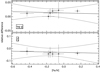 |
Fig. 5 Relative difference between the seismic and dynamic parameters as a function of stellar metallicity for the solar-calibrated surface gravity (top) and mean stellar density scaled from Δνcor (bottom). Solid and dotted lines indicate a linear fit and the corresponding 95% confidence intervals, respectively. |
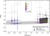 |
Fig. 6 Seismic masses for a sample of halo and thick-disk stars as a function of stellar metallicity. The open grey symbols show the original values taken from Epstein et al. (2014). Black symbols correspond to masses from the classical scaling relations as done by Epstein et al. (2014), but based on Δνc determined from the full Kepler data sets. Coloured symbols show the masses based on our re-calibrated scaling relations, where the colour indicates the observed large frequency separation Δνc. The grey-shaded bars indicate the expected mass based on the high age and low metallicity constraints for these stars (Epstein et al. 2014). |
4.3 The benchmark case HD 185351
Since Kepler red giants usually lack accurate non-seismic parameters, it is difficult to independently verify our newly established non-linear scalings. A rare example where this is nevertheless possible is the bright (V = 5.18) RGB star HD 185351 observed with Kepler, for which Johnson et al. (2014) determined a precise radius from interferometry and spectral energy distribution fitting (see Table 3). Sharma et al. (2016) used the star as a benchmark case in theiranalysis as well and found a seismic radius that overestimates the interferometric values by about 5 ± 4%. Our non-linear scalings (for νmax and Δνc) reduce the discrepancy to about 2.1 ± 3.2% if we use the original global seismic parameters from Johnson et al. (2014) as input. Even though the star is very bright the Kepler observations of HD 185351 are quite noisy and reveal significant modes only in the central three to four radial orders of the pulsation power excess. We can therefore only determine Δνc. Based on this the radius discrepancy reduces to 1.7% ± 3.6%. We further note that our non-linear scalings give a mass of 1.72± 0.14 M⊙, which is in good agreement with the value of 1.6 M⊙ found by Hjørringgaard et al. (2017) based on a detailed seismic analysis.
Non-seismic and seismic radius of the bright RGB star HD 185351 observed by Kepler in short-cadence mode.
5 Cluster stars
Using the dynamic fundamental parameters of a sample of eSB2 binaries, we have established new non-linear seismic scaling relations. The calibration sample is, however, quite small covering only a small range of evolutionary stages (~7.6–14 R⊙) and is limited to RGB stars, burning hydrogen in a shell around an inert helium core. In order to test our scaling relations beyond this limitation, we need a larger sample of stars covering various evolutionary stages, including stars in the red-clump (RC) phase of quiescent core-helium burning, with homogenous seismic measurements and additional accurate non-seismic constraints. The Kepler observations of the red giants in the two well-studied open clusters NGC 6791 and NGC 6819 form such a sample.
5.1 NGC 6791
The cluster NGC 6791 is one of the oldest and at the same time most metal-rich open clusters known (e.g. Carretta et al. 2007). It is a well-populated cluster, with a significant number of stars at basically all stages of evolution from cool main-sequence stars to white dwarfs (e.g. King et al. 2005; Bedin et al. 2005) including many variable stars (e.g. Mochejska et al. 2002; de Marchi et al. 2007). Despite the large number of studies there is little agreement on its age, ranging from 7–12 Gyr, and metallicity because of correlated uncertainties in distance, reddening, and metallicity, with the latter ranging from [Fe/H] = +0.29 (Brogaard et al. 2011) to +0.45 (Anthony-Twarog et al. 2007). It seems likely that the differences are mainly caused by differences in the adopted reddening, with typical values of either E(B−V) = 0.09 (Stetson et al. 2003) or 0.15 (an average of literature determinations, Carretta et al. 2007). An et al. (2015) carefully calibrated the cluster’s colour-magnitude diagram (CMD) and report a true distance modulus (DM) of  mag and an age of 9.5 ± 0.3 Gyr from isochrone fitting, where the latter uncertainties do not cover systematic uncertainties in the isochrones. A detailed literature overview can be found in Wu et al. (2014b).
There are several studies available (Basu et al. 2011; Miglio et al. 2012; Wu et al. 2014a,b) that aimed to constrain the RGB mass and true DM from Kepler photometry of red giants in NGC 6791. Even though these studies are different in detail they converge to MRGB = 1.23 ± 0.02 M⊙ and  mag. Brogaard et al. (2012), on the other hand, suggested a slightly lower RGB mass of 1.15 ± 0.02 M⊙ based on isochrone fitting to the mass and radius of several eclipsing binaries on the main sequence of NGC 6791. Miglio et al. (2012) furthermore found a small but significant difference between the average mass of RGB and RC stars of
  , indicating only moderate mass loss for this metal-rich cluster.
5.2 NGC6819
The cluster NGC 6819 is a very rich open cluster with roughly solar metallicity of [Fe/H] = + 0.09 ± 0.03, reddening E(B−V) = 0.14 ± 0.04 (Bragaglia et al. 2001), and age of about 2.5 Gyr (isochrone fitting in the CMD; e.g. Kalirai & Tosi 2004). Since there is reasonable agreement on the metallicity and reddening of NGC 6819 it has been used to study other phenomena such as the initial-final mass relation using the cluster’s white dwarf population (e.g. Kalirai et al. 2008). Jeffries et al. (2013) reported, however, that the detached eclipsing binary KIC 5113053, located near the cluster turnoff, is significantly older than the commonly adopted cluster age. They fit the mass and radius of the binary components with isochrones from various stellar evolution codes and find ages ranging from 2.9 to 3.7 Gyr while the same isochrones give values between 2.1 and 2.4 Gyr for fits in the CMD. This clearly indicates that the age determination of stellar clusters is still problematic and obviously quite model-dependent. As for NGC 6791, Basu et al. (2011) used the Kepler photometry to determine the RGB mass and true DM of NGC 6819 to MR GB = 1.68 ± 0.03 M⊙ and  mag, which is again compatible with the estimates of 1.75 ± 0.03 M⊙ and 11.88 ± 0.14 mag reported by Wu et al. (2014a,b). Miglio et al. (2012) found no mass loss on the cluster’s giant branch but a smaller RGB mass of 1.61± 0.04 M⊙, which is supported by Sandquist et al. (2013) who expected MRGB to be about 8% smaller than reported based on isochrone fitting to the mass and radius of EBs on the cluster’s main sequence.
5.3 Input parameters
5.3.1 Global seismic parameters νmax and Δνcor
A prerequisite for the subsequent analysis is that the stars of interest are members of the clusters. As a starting point we use the list of “seismic members” from Stello et al. (2011) from which we exclude misclassified stars, suspected binaries, and stars with other “peculiarities” (e.g. Corsaro et al. 2012; Bellamy & Stello 2015). The about 1420-days-long Kepler time series of the remaining cluster members are processed in the same way as the G16 sample (see Sect. 3). In a first step, we extract νmax and Δνc from the power density spectra of all stars and find values with sufficient accuracy for 51 and 39 stars in NGC 6791 and NGC 6819, respectively. They are shown in Fig. 7a, where they form two slightly different sequences indicating the different RGB masses of the clusters (e.g. Hekker et al. 2011). To disentangle RC stars from RGB star, we compute the phase shift of the central radial mode (ϵc; see Fig. 7b). According to Kallinger et al. (2012) and Christensen-Dalsgaard et al. (2014), ϵc is expected to be significantly smaller for RC stars than for RGB star at a given Δν. Unlike what Handberg et al. (2017) claim for stars in NGC 6819, we can in fact unambiguously identify the evolutionary stage of almost all stars with this method. Only for two stars in NGC 6819 (KIC 5023931 and KIC 5111940) the result remains uncertain. A visual inspection of their dipole mode spectrum does, however, reveal that both stars are very likely RGB stars (which is confirmed by the stars’ positions in the seismic colour-magnitude diagram; see Sect. 5.3.3 and Fig. 9). The two stars are not part of other RGB-RC classification analyses (e.g. Vrard et al. 2016; Elsworth et al. 2017; Hon et al. 2017).
Subsequently, we try to peakbag the radial mode frequencies for all stars in order to determine the curvature- and glitch-corrected large separation Δνcor (see Sect. 3.4). However, we are only able to measure Δνcor with sufficient accuracy for 32 out of 51 NGC 6791 members and 34 out of 39 NGC 6819 members. The corresponding curvature parameters α are given in Fig.7c, showing a large intrinsic scatter between the two clusters, presumably due to a mass and/or metallicity dependency. We also see that the overall trend significantly deviates from that provided by Mosser et al. (2013). In order to avoid losing a significant number of stars for the subsequent analysis, especially at low Δν, we use a different method to determine Δνc.
Our original approach to extract Δνc is based on fitting a sequence of Lorentzian profiles to the power density spectrum that cover the l = 0 to 2 modes in the three radial orders around the central radial mode. We now extend the range to five radial orders and add a curvature term to the parameterisation of the radial mode frequencies according to Eq. (4), rather than treating them as equidistant as in the original approach. To test if the resulting Δνcor are sufficient for the subsequent analysis, we compare them to Δνcor determined from Eq. (6) for the stars for which we could successfully peakbag the radial modes in Fig. 7d. We find that the individual values agree with each other within ~0.30% on average, which is not much larger than the average uncertainty of their ratio of ~0.25%. This indicates that a remaining glitch contribution to Δνcor as determined from Eq. (4) is quite small and essentially covered by the uncertainties delivered by MULTINEST. We therefore assume Δνcor from Eq. (4) to be precise enough for the subsequent analysis.
Finally, we show the ratio Δνc∕Δνcor in Fig. 7e. This indicates that Δνc is a good representation of the “true” Δν for the least evolved RGB stars (large Δν) but the curvature and glitch contribution systematically increases for more evolved RGB stars. For RC stars, Δνc includes a significant contribution from curvature and glitches that is much larger than the observational uncertainties, which needs to be corrected if one is interested in the real large separation. More details about the curvature and glitch signal will be presented in a separate study (Kallinger et al., in prep.).
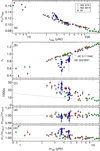 |
Fig. 7 Global seismic parameters for NGC 6791 and NGC 6819, where the RGB stars are indicated by green circles and red triangles, respectively, and the RC stars of both clusters by blue symbols. Grey-filled squares show the EBs from Sect. 2. Panel a: ratio of Δνc and νmax; panel b: the phase shift ϵc of the central radial mode. The vertical dashed lines indicate the median large separations of RC stars in the two clusters. Panel c: curvature term α. Panel d: ratio of Δνcor computed in different ways (Eqs. (4) and (6)); panel e: ratio of central large separation and Δνcor computed according to Eq. (4). The dashed lines in panels c, d, and e indicate the scaled curvature term from Mosser et al. (2013) and unity, respectively. |
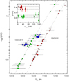 |
Fig. 8 Peak frequency vs. effective temperature for our sample of RGB (red and green symbols) and RC (bluesymbols) stars in NGC6791 and NGC6819, respectively. Circles and squares indicate stars with theeffective temperature taken from the APOKASC catalogue and derived from polynomial fits (greydashed and dotted lines), respectively. Horizontal grey lines represent the uncertainties in Teff. The inset shows the metallicity measurements from the APOKASC catalogue along with the average values (dashed lines) and their uncertainties (dashed-dotted lines). |
 |
Fig. 9 Average apparent bolometric magnitude as a function of νmax (left panel) and Δνcor (right panel) for our sample of RGB (red and green dots) and RC (blue dots) stars in NGC 6791 and NGC 6819, respectively. The dotted lines in the left panel (and top inset in the right panel) correspond to BaSTI isochrones (Z = 0.03 and 8.0 Gyr for NGC 6791 and Z = 0.02 and 2.5 Gyr for NGC 6819) arbitrarily shifted to match the observations. The loops in the isochrones correspond to the various phases of the RGB evolution. Solid lines in the right panel indicate polynomial fits to the RGB stars. The bottom inset gives the mass of the BaSTI isochrones normalised to the mass at νmax =100 μHz. |
5.3.2 Effective temperatures
The cluster stars’ effective temperatures are taken from the APOKASC catalogue (DR13; Pinsonneault et al. 2014). Unfortunately, only about half of our sample stars are listed in the catalogue. For stars with near-equal mass, however, we can expect a tight relation between νmax and effective temperature. As shown in Fig. 8, there is a clear relation, so that we can fit Teff as a function of log νmax, for which we use first (RGB) and second order (RC) polynomial fits. Effective temperatures for the remaining stars are then determined from the fits according to their νmax. Figure 8 also shows that the uncertainties listed in the APOKASC catalogue (typically about 80–90 K) are significantly larger than the scatter around the fits. This is because the APOKASC errors are supposed to also cover systematic uncertainties. In our analysis we are more interested in random errors and therefore adopt uncertainties for all stars that correspond to the root mean square (rms) scatter around the fits, which is ±24 (RGB) and ±21 K (RC) for stars in NGC 6791, and ±16 (RGB) and ±27 K (RC) for stars in NGC 6819). Hence we assume any systematic Teff errors are the same for all red giants. The average metallicities ([M/H]) for the stars listed in the catalogue are + 0.38 ± 0.05 for NGC 6791 and + 0.05 ± 0.04 for NGC 6819, which is in good agreement with previous measurements.
5.3.3 Stellar luminosities
Stellar luminosities are usually determined by the apparent magnitude of a star and its distance but to derive distances is a difficult task. Several classical studies of the two clusters revealed distance moduli that diverge by up to half a magnitude. The situation improved with the availability of precise global oscillation parameters from Kepler, which improved the uncertainties to about 0.1–0.15 mag. This implies that the luminosity of individual cluster stars cannot be determined to better than about 10%–12%, which makes them impractical for our test of the seismic scaling relations.
However, the fact that the cluster members are equally distant4 and that their light undergoes approximately the same reddening and extinction enables us to derive relative luminosities that depend only on the differences between the apparent bolometric magnitudes (mb ol) of the individual stars. Red giants are brightest in the near-infrared so that the 2MASS JHK photometry (Skrutskie et al. 2006) is well suited to determine accurate mbol. We bolometrically correct the individual interstellar extinction corrected 2MASS magnitudes by interpolating Teff, log g, and metallicity in the tables of Bonatto et al. (2004), where the surface gravity is estimated from 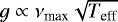 . The uncertainties of all parameters are fully taken into account and the final apparent bolometric magnitude (and its uncertainty) is computed from the average of the three individual values.
In Fig. 9 we show mbol as a function of νmax and Δνcor. These seismic colour-magnitude diagrams (sCMD) are a powerful tool for the characterisation of cluster stars. All stars that are single members are supposed to follow a distinct sequence (indicated here by BaSTI isochrones; Pietrinferni et al. 2004). If a star, assumed single, falls below the sequence, this clearly indicates a background star. If a stars falls above the sequence, it is either a foreground star or an unresolved binary combining the light of more than one object. In the present case, the membership analysis (Stello et al. 2011) was already done carefully enough so that all stars in our sample are clearly cluster members. Additionally, the sCMD does even allow us to distinguish between RGB and RC stars. The effect is slightly smeared out when taking νmax as a reference but for Δνcor, RGB and RC stars are clearly separated. This is not surprising because RC stars are slightly hotter (see Fig. 8) and therefore, more luminous than RGB stars with the same Δνcor. We note that the actual identification used here is based on the phase shift of the central radial mode (Kallinger et al. 2012) and therefore, entirely independent.
Linear fits in the mbol − logΔνcor plane to the RGB stars reveal that the apparent bolometric magnitudes are accurate to about 0.02 mag for both clusters. This implies that we can constrain the relative luminosities to about 1.8%, which is at least five times more accurate than the absolute luminosities.
5.3.4 Stellar masses
In a cluster in which all stars have the same age and primordial chemical composition, there is a tight relation between the initial mass of a star and its evolutionary stage, with more massive stars being further evolved. On the giant branch, however, stars evolve quickly, compared to main-sequence stars, so that high-luminosity RGB stars are expected to be only slightly more massive than low-luminosity RGB stars. This is shown in the inset of Fig. 9, where we indicate how mass is expected to change along the giant branch. According to BaSTI isochrones (which include mass loss using the Reimers (1975) formulation with the free parameter η set to 0.2) the RGB star mass in NGC 6819 is supposed to increase by about 1% from the least evolved to the most evolved star in our sample. Such high sensitivity to mass is also observed in the binary system KIC 9163796, which consists of a sub giant and a red giant with a mass ratio of 1.01 ± 0.01 (Beck et al. 2018b). For NGC 6791 the mass dispersion is even smaller as the evolutionary mass increase is balanced by mass loss (based on η = 0.2). It is therefore safe to assume that all RGB stars in our sample have approximately the same mass, MR GB.
5.4 Comparison of observed and computed global seismic parameters for RGB stars
With independent constraints for the mass, effective temperature, and luminosity in hand, we can now compare the global seismic parameters estimated from scaling relations to the actual observed ones.
5.4.1 Testing the νmax-scaling
Given Eq. (2) and L ∝ R2T4, the peak frequency νmax scales as
 (9)
(9)
The solar-scaled luminosity can be determined according to
 (10)
(10)
where the factor 79.829 comes from the absolute bolometric magnitude of the Sun,  = 4.7554 mag (Kopp & Lean 2011). By combining the above equations, we can write the logarithmic peak frequency, log νmax,cal, as
 (11)
(11)
where νmax,cal, M, and Teff are in solar units. This description of the peak frequency is independent of any seismic constraint and corresponds to the right-hand side of Eq. (9).
If the νmax -scaling were correct, νmax,cal would linearly scale with the observed peak frequency. This can be tested by fitting a function
 (12)
(12)
to the RGB stars of both clusters, where the slope k would need to be equal to one if the scaling is linear. We show νm ax,cal as a function of the observed peak frequency along with the best fit in Fig. 10. We find a best fit of k = 0.989 ± 0.004 for NGC 6791 and 0.995 ± 0.004 for NGC 6819. A possible explanation for k≠1 are potential systematic uncertainties in the adopted effective temperatures. However, it turns out that we need to subtract about 400 (NGC 6791) and 250 K (NGC 6819) to obtain slopes that are consistent with one. Such large systematics do not seem very likely. A reconciliation can be obtained by assuming a non-linear scaling of the form  , where κ = 1∕k. The slopes from above translate into exponents of 1.010 ± 0.004 and 1.005 ± 0.004, which are consistent with the value of 1.008 ± 0.002 determined from the eSB2 stars in Sect. 4. Combining the three independent cluster and eSB2 measurements gives an average value of κ = 1.0075 ± 0.0021. We also tested higher-order polynomial fits instead of Eq. (12) but found them to be statistically insignificant.
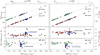 |
Fig. 10 Top panels: mbol and Teff scaled νmax,cal (left) and Δνcor,cal (right) as a function of the observed parameters for the sample of RGB (red and green dots) and RC (blue dots) in NGC 6791 and NGC 6819, respectively. The dashed lines indicate linear fits (in log-log scale) to the RGB stars, which correspond to power-law fits in linear scale. The panels are plotted upside down so that bright stars are at the top. Middle and bottom panels: residuals to the fits. The blue dashed lines indicate the average offset of RC stars with the mean valuesand rms scatter given. |
5.4.2 Testing the Δνcor-scaling
As for the peak frequency, we can express the large separation as a function of M, L, and Teff according to
 (13)
(13)
which translates into a logarithmic description as
 (14)
(14)
We then again test the linearity of the Δνcor-scaling by fitting the function
 (15)
(15)
to the RGB stars in NGC 6791 and NGC 6819. As we might expect, we find k with 0.981 ± 0.003 and 0.980 ± 0.004, which differs significantly from unity in both clusters. The excellent agreement between the two slopes indicates again that the Δν-scaling is not affected by metallicity; at least not beyond 0.1%−0.3% in the Teff range for which Kepler has observed red giants in the two clusters.
Unlike for the exponent in the νmax-scaling, the slope k in Eq. (15) cannot be directly translated into the parameter γ of the non-linear Δν-scaling presented inEq. (8). It is, however, evident that the cluster stars also support a non-linear scaling, and replacing Δνcor,⊙ in Eq. (15) by Δνcor,⊙[1 − γlog2(Δνcor,obs∕Δνcor,⊙)] basically linearises the Δν-scaling (meaning k ≃ 1) if we adopt the original value of γ = 0.0085.
5.5 Extending the scalings to RC stars
So far we have only considered RGB stars and from the middle and bottom panels of Fig. 10 it is evident that the scaling relations cannot be directly applied to RC stars. For the peak frequency, subtracting the linear fits from all stars results in a median underestimation of logνmax of 0.033 ± 0.012 for the clump stars in NGC 6791, while no systematic deviation is found for the RC stars in NGC 6819. The obvious explanation for this is mass loss in NGC 6791. The offsets d in the fits represent the RGB mass and distance moduli of the two clusters. Since the distance is practically the same for all cluster members, a systematic difference between the fit and RC stars can only mean that the mass is different between RGB and RC stars. In fact, we can estimate that MRC∕MRGB = 10−0.033±0.012. Or, in other words, the RC stars in NGC 6791 have lost 7.5% ± 2.5% of their mass between the late RGB and clump phase, which is in agreement with, but determined more accurately than, the findings of Miglio et al. (2012).
Subtracting this mass loss for clump stars in Eq. (14) leads to an median overestimation of log Δνcor of − 0.018 ± 0.009 for clump stars in NGC 6791, which is in agreement with the value of − 0.018 ± 0.005 found for NGC 6819. Because we find the same systematic difference in both clusters, this indicates that the Δν-scaling should be different for RC stars. From the average value we can estimate a correction factor of 1.04 ± 0.01 (i.e. 100.018±0.05) for the large separation of clump stars, which is slightly larger than the value suggested by Miglio et al. (2012). From this we can finally formulate our new non-linear seismic scaling relations as
 (16)
(16)
![\begin{equation*}\sqrt{\bar\rho} = \frac{{{\mathrm \Delta}}\nu_{\mathrm cor} }{ {{\mathrm \Delta}}\nu_{\mathrm cor,\odot}} \left [\eta - (0.0085\pm0.0025) \cdot \log^2 ({{\mathrm \Delta}}\nu_{\mathrm cor} / {{\mathrm \Delta}}\nu_{\mathrm cor,\odot}) \right ]^{-1}, \end{equation*}](/articles/aa/full_html/2018/08/aa32831-18/aa32831-18-eq46.png)
where g, Teff, and  are in solar units, νmax,⊙ = 3140 ± 5 μHz and Δνcor,⊙ = 135.08 ± 0.02 μHz, and η is equal to one in the case of RGB stars and 1.04 ± 0.01 for RC stars.
5.6 Seismic fundamental parameters from grid modelling
We implement the new non-linear scalings into the grid-modelling approach from Kallinger et al. (2010a), which compares the observed νmax and Δνcor with those of an extensive grid of stellar models where the model seismic parameters are determined from the scaling relations. The grid consists of canonically solar composition-scaled BaSTI isochrones (Pietrinferni et al. 2004, version 5.0.0) with mass-loss parameter η = 0.2. The grid covers more than four million models from the sub-giant phase to the asymptotic giant branch (AGB) with initial masses ranging from 0.5 to 4 M⊙ and chemical compositions of (Z, Y) = (0.0003, 0.245) to (0.4, 0.303) with typical increments in Z of 0.001. The Bayesian comparison between observed and model parameters fully accounts for all observational uncertainties including those of the scaling relations, and can use prior information for all model parameters including the evolutionary stage.
Unfortunately, our algorithm can only treat stars one by one independently and not as an ensemble with common age and chemical composition. To mimic such an ensemble analysis, we first run our grid modelling using only νmax, Δνcor, Teff, and the evolutionary stage but no prior information on the chemical composition and age of the stars. Even though the resulting best-fit models group around specific metallicities and ages for each cluster, the scatter is still quite large. To improve this we then use the median metallicity (Z = 0.033 for NGC 6791 and 0.020 for NGC 6819) and age (10.1 and 2.9 Gyr) found in the first run as priors for a second run, where we use Gaussian priors with a σ of 10%. The resulting best-fit model masses and radii and their uncertainties are shown in Fig. 11. As expected the new seismic masses are incompatible with previous estimates from linear scalings and settle at values that are 10%–15% lower than reported by others.
For NGC 6791 we find the stars to group around MRGB = 1.10 ± 0.03 and MRC = 1.02 ± 0.05 M⊙. The scatter is comparable with the average uncertainties of the individual measurements. Even though our MR GB is significantly smaller than found by others, the mass loss of ΔM = MRGB − MRC = 0.08 ± 0.03 M⊙ is in perfect agreement with that found by Miglio et al. (2012), who inferred a mass-loss parameter of η = 0.1−0.3. The good agreement isnot surprising because the non-linear effects in our scaling relations in practice cancel out when computing the mass difference of stars with similar νmax and Δν. Furthermore we note that the observed mass loss is consistent with that of BaSTI isochrones with η = 0.2 (see Fig. 11).
The situation is less straightforward for NGC 6819, for which we find less good agreement between masses of the individual cluster members. We find an average of MRGB = 1.45 ± 0.06 M⊙, and a scatter about twice as large as the average uncertainty of the individual measurements. A possible explanation for this extra scatter could be the presence of more than one generation of stars. To verify this, however, is beyond the scope ofthe present analysis. Also the RC stars scatter about twice as much around the average mass MRC = 1.54 ± 0.07 M⊙ than expected from their individual uncertainties. This might be due to the fact that our BaSTI models imply a mass loss between the RGB and RC phase, which leads to overestimation of the mass for RC stars if they do not undergo mass loss in reality. This effect is, however, small (~2%) as can be seen from the isochrones in Fig. 11 and is therefore within the uncertainties of our analysis.
As a consistency check we also compute M and R directly from the non-linear scaling relations and find them to generally agree with the values from grid modelling but with larger uncertainties (see Fig. 11). A summary of the cluster parameters determined from grid modelling is given in Table 4. In Fig. 11 we also show the stars’ positions in the HR-diagram based on the output of our grid modelling.
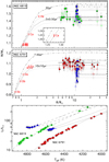 |
Fig. 11 Seismic mass vs. radius from grid modelling (filled circles) and direct computations from scaling relations (open circles) based on νmax and Δνcor (from Eq. (4)) as seismic input. Symbol colours are the same as in Fig. 10. Also plotted are BaSTI isochrones (dotted, dashed, and dashed-dotted lines) for solar metallicity in the top panel and [Fe/H] = 0.26 in the bottom panel with the numbers indicating the age of the isochrones as well as a number of eclipsing binaries (red squares), with the labels indicating: Aa → WOCS23009 A; Ba, Bb → WOCS24009 A & B; Ca, Cb → WOCS40007 A & B; Da, Db → V18 A & B; Ea, Eb → V20 A & B; Fa → V80 A. The inset in the top panel zooms onto the position of the primary component of WOCS40007 (Ca). The bottom panel shows the star’s position in the HR-diagram along with a 3 (dotted line) and 10 Gyr (dashed line) BaSTI isochrone for NGC 6791 and NGC 6819, respectively. |
RGB mass, mass loss, true distance modulus, and age for both clusters from selected sources in the literature and determined in the present analysis (based on the non-linear scalings with νmax and Δνcor as seimic input).
5.7 Cluster distance moduli
There are several ways to determine the cluster’s distance moduli from the seismic observations. One could use the constants d in Eqs. (12) and (15), which represent the mass and true distance modulus terms in the calculated peak frequency (Eq. (11)) and large separation (Eq. (14)). However, a more direct way is to combine Eqs. (11) and (14) in order to express the true distance modulus as
 (18)
(18)
where νmax and Δν are scaled according to Eqs. (16) and (17), respectively. From that we find average true distance moduli of  (NGC 6791) and 11.91 ± 0.03 mag (NGC 6819), where the uncertainties represent the spread of the individual values (and not the actual error of the mean, which would be about five times smaller). Our distance moduli are in agreement with, but more precise than, previous seismic and non-seismic determinations and translate into distances of 4.19 ± 0.06 kpc (NGC 6791) and 2.41 ± 0.03 kpc (NGC 6819).
5.8 Cluster ages
A direct consequence of the fact that the classic seismic scaling relations overestimate the mass of red giants is that they significantly underestimate their ages. With our non-linear scaling relations implemented in the grid modelling we measure the ages to be 10.1± 0.9 for NGC 6791 and 2.9 ± 0.3 Gyr for NGC 6819, which is about 30% older than reported from previous seismic analyses. In principle, any age determination suffers from various sources of uncertainties. For example, the isochrone fiting to an observed CMD, which are frequently used to estimate cluster ages, suffer from the usual difficulties of measuring interstellar reddening or extinction and the transformation of the model parameters into observable colours. A more robust and direct method is to compare the mass and radius of isochrones to those of EB cluster members.
There are a number of known EB members in NGC 6791. Grundahl et al. (2008) carried out a detailed analysis of the system V20 with one component located close to the cluster turnoff. This allowed them to measure the cluster age to better than a few per cent within a given set of isochrones. They did, however, also find that the actual age largely depends on the chosen set of isochrones, and hence reported an age ranging from 7.7–9 Gyr, with the latter estimate coming from BaSTI isochrones. The reason for this ambiguity might be due to the high metallicity of the cluster or due to the role convective overshoot plays in the morphology of isochrones near the turnoff. Brogaard et al. (2011, 2012) used two additional binary systems (V18 and V80). They find that isochrones that are required to fit the EBs in the mass-radius diagram as well as in the clusters colour-magnitude diagram give a best fit (within their set of Victoria isochrones) for an age of 8.3 ± 0.5 Gyr, which corresponds to a mass on the lower RGB of 1.15 ± 0.02 M⊙. Brogaard et al. (2016) further measured the mass of the giant component of the EB V9 to be 1.14± 0.02 M⊙, which is again more compatible with our MRGB than with that from previous seismic analyses.
We do not perform isochrone fitting but exemplarily show isochrones in Fig. 11that correspond to the result of our grid modelling. In fact, the EBs are more consistent with a 10 ± 1 Gyr age-range than with previous seismic age estimates and therefore, support the low RGB mass.
Cluster NGC 6819 also includes a number of known detached eclipsing binary systems (e.g. Jeffries et al. 2013; Sandquist et al. 2013; Brewer et al. 2016), most notably WOCS 24009 and WOCS 40007, whose components are all located at the upper main sequence of the cluster (1−1.25M⊙; see Fig. 11). The most massive and therefore most age sensitive star amongst them is WOCS 40007 A. Jeffries et al. (2013) determined an age of 3.1 ± 0.4 Gyr from isochrone fitting to the well-defined mass and radius of the star. Even though this estimate is affected by systematic uncertainties it is quite clear that the real age of the star exceeds the commonly adopted age of the cluster of 2− 2.5 Gyr. A potentially even more age sensitive star is WOCS 23009 A, which is located near the cluster’s turnoff. Brewer et al. (2016) used all measured EBs to determine a cluster age of 2.4 ± 0.2 Gyr. However, this result relies mostly on the mass of WOCS 23009 A, which might be questioned because the very low-mass companion hampers a dynamic mass estimate. Instead, its mass was determined from the isochrones used to constrain the cluster age. We argue that this represents a circular argument, so that the star should be excluded from the analysis. As can be seen from Fig. 11, the remaining binaries are in favour of the older isochrones and therefore support the low RGB mass of about 1.45 M⊙ instead of the previously reported 1.61−1.75 M⊙.
Following the findings of Grundahl et al. (2008), we note that it might well be that our cluster ages from BaSTI isochrones mark more an upper limit than an accurate determination. In this context we note that Stancliffe et al. (2016) have shown that solar evolutionary tracks from various stellar evolution codes differ by up to 150 K when leaving the main sequence at significantly different ages, with BaSTI providing the oldest models. It is therefore not surprising that the two clusters’ ages are still a matter of debate. However, to solve this is beyond the scope of the present analysis.
5.9 Metallicity dependence
With the true distance modulus and mass available we can directly compute Δνcor,cal from Eq. (14) using the linear scaling relations and compare it to the observed values. This is shown in Fig. 12a, where we plot the ratio between the observed and calculated large separation as a function of effective temperature. As suggested from models by White et al. (2011), we do indeed find a trend that the scaled large separation increasingly overestimates the observations towards lower effective temperature on the RGB. However, our uncertainties are too large to reveal a potential dependence of this trend on metallicity as suggested by the models. We can therefore neither confirm nor disprove any metallicity influence on the large separation. We do, however, show in Fig. 12b that this trend is well reproduced by the non-linear  scaling, without the need to incorporate the stellar metallicity.
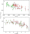 |
Fig. 12 Ratio of observed and calculated (see Eq. (14)) large separation for RGB stars in NGC 6791 (red circles) and NGC 6819 (green circles). Panel a: this ratio as a function of the effective temperature along with the expected values from Guggenberger et al. (2016) (diamond symbols). Panel b: the ratio as function of Δν along with non-linear scaling of the solar reference (solid line), that is, the term in square brackets of Eq. (17). |
6 Implications for the APOKASC sample
Apart from the consequences for the cluster ages and RGB masses shown above, our new scaling relations will also impact the seismic fundamental parameter determination of other red giants. A prominent set of red giants that is currently being vigorously investigated is the so-called APOKASC sample (e.g. Elsworth 2017). APOKASC is a collaboration between APOGEE’s spectroscopic survey in the near infrared at Apache Point (SDSS) and the Kepler Asteroseismic Consortium (KASC) for the study of cool stars in the Kepler field that aims to take advantage of the high-quality spectroscopic and asteroseismic data to derive precise fundamental parameters for a large number of stars. The resulting catalogue includes about 6600 red giant stars (Pinsonneault et al. 2014), which are spectroscopically and asteroseismically characterised. Among those, we can determine the curvature- and glitch-corrected large separation Δνcor (see Sect. 3.4) with sufficient accuracy (the median uncertainty is about 0.13%) from the radial mode spectrum of about 5100 stars. Details of the mode fitting and the curvature and glitch analysis are the subject of a separate paper (Kallinger et al., in prep.) and initial results about the associated mode amplitudes and line widths are given by Vrard et al. (2018).
We then use the grid-modelling approach described in Sect. 5.6 to determine the seismic masses and radii from the νmax, Δν cor, Teff, and evolutionarystage measurements of these stars. To study the implications of the non-linear scalings on the mass and radius distributions of red giants in the Kepler field, we computed the seismic masses and radii twice: once based on the original seismic scalings andonce based on our new non-linear scalings. The results are shown in Fig. 13. While the radius distribution is basically unaffected, we find a significant shift towards lower masses in the mass distribution. Interestingly, this shift is largely caused by the RGB stars in the sample. Whereas the distribution of core-He burning stars (red clump and secondary clump stars) is relatively unaffected, the peak in the distribution of RGB stars shifts from the 1.3−1.4 M⊙ bin to the 1.1−1.2 M⊙ bin when implementing the non-linear seismic scalings instead of the original linear scalings in the grid modelling. Numerical tests show that the reason core-He burning stars are basically unaffected is because the “non-linear effect” in the Δν-scaling is partly compensated for by the correction factor η (which is different from one for core-He burning stars).
The approximately 15% shift in mass for RGB stars cannot be explained by the uncertainties of the individual measurements, which are on the order of 5%. It is therefore a real effect and should be of particular interest for future Galactic archeology studies (such as Anders et al. 2017; Stello et al. 2017), which attempt to use seismic mass and radius distributions of different parts of the Milky Way to study the structural and chemical evolution of our Galaxy.
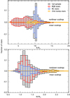 |
Fig. 13 Radius (top panel) and mass (bottom panel) distributions of about 5100 red giants from the APOKASC sample computed from grid modelling based on our new non-linear scalings with νmax and Δνcor as seismic input (upwards pointing) and the classical linear scalings (downwards pointing). The full sample and subsamples corresponding to the different evolutionary stages are shown by grey and coloured bars, respectively. |
7 Summary
In recent years the seismic scaling relations for νmax and Δν have become increasingly important in various fields of astrophysics because they can be used to estimate the mass and radius of stars showing solar-like oscillations. With the high-precision photometry of Kepler, the uncertainties in the seismic observables are now small enough to estimate masses and radii with a precision of only a few per cent. Even though this seems to work quite well for main-sequence stars, there is empirical evidence, mainly from studies of eclipsing binary systems, that the seismic scaling relations systematically overestimate the mass and radius of red giants by about 5% and 15%, respectively.
Various model-based corrections to the Δν-scaling reduce the problem but do not solve it. Furthermore, such corrections suffer from systematic errors in the models, which clearly affect the models’ large frequency separation but which are not accounted for in the corrections. It is therefore, not yet clear whether these corrections are of any physical relevance for the Δν-scaling or are simply the consequence of the systematic errors in the models.
Our goal was therefore to revise the seismic scaling relations in order to account for the known systematic mass and radius discrepancies in a completely model-independent way. This can be done best by comparing the dynamic and seismic fundamental parameters of eclipsing binaries hosting at least one star with detectable solar-like oscillations. So far there are six such systems known, with measurements accurate enough for a conclusive analysis. To minimise potential biases in the dynamic parameters we used the results from three different groups (Gaulme et al. 2016; Brogaard et al. 2018; Themeßl et al. 2018) based on different instrumentation and analysis methods. We used probabilistic methods to re-examine the global oscillation parameters of the giants in the binary systems. From this we determined the corresponding seismic fundamental parameters and found them to agree with the dynamic parameters if we adopt non-linear seismic scaling relations. Even though the sample is quite small, the Bayesian evidence is clearly in favour of the new non-linear scalings. We also found that the results are best when using a curvature- and glitch-corrected large separation as input for the Δν-scaling.
We then compared the seismic parameters of about 60 red giants observed by Kepler in two open clusters to those scaled from independent measurements and found the same non-linear behaviour as for the eclipsing binaries. Our final proposed scaling relations (Eqs. (16) and (17)) are based on both samples (eclipsing binaries and cluster stars) and cover a broad range of evolutionary stages from RGB stars to core-helium-burning red clump stars.
It has been suggested that at least the Δν-scaling should in some sense be sensitive to stellar metallicity. We found that our samples were too small and/or not accurate enough to prove or disprove such a metallicity dependency. On the other hand, we could show that a previously claimed “metallicity effect” that was made responsible for the discrepancy between seismic and independent estimates of the mass of some highly evolved (luminous) halo and thick-disk stars can be equally well explained with our (metallicity-independent) non-linear scalings. The difference between the previous linear and our new non-linear relations increases towards more luminous stars.
A directconsequence of the new scaling relations is that the average mass of stars on the ascending giant branch in both investigated clusters reduces on average by about 12%, allowing us to revise the clusters’ true distance moduli and to conclude that both clusters are older than suggested by previous seismic investigations. We further note that independent estimates of the masses and radii of several eclipsing binaries located before or close to the turnoff in both clusters are more consistent with our new MRGB measurements than with those based on linear scaling relations. Apart from its scientific value, we interpret this as another indication that our revised scaling relations provide more realistic estimates of the mass and radius of a red giant than the classical relations.
We also checked how the revised scalings affect the mass and radius distributions of red giants in the full Kepler field, which is an input for galactic archeology studies. We found that while the radius distribution is largely unaffected, the mass distribution changes significantly, which is predominantly caused by an approximately 15% reduction of the mass distribution of RGB stars.
The revised seismic scaling relations presented here are most likely still a simplification of the intrinsic relation between the seismic quantities and the fundamental parameters of a star. To check and potentially improve this would require large samples of stars with accurate seismic and independent measurements of their fundamental parameters, which are currently not available. The original Kepler field does not include many more eclipsing binaries and is therefore insufficient for such an analysis. Observations with the K2 mission (Howell et al. 2014) might reveal new systems but their seismic observables are not accurate enough. We might expect some improvements (in the sense of Huber et al. 2017) from future Gaia data releases for stars in the original Kepler field but these stars lack independent mass constraints. More promising in the near future are the observations with one-year coverage near the ecliptic poles by the Transiting Exoplanets Survey Satellite (TESS; Ricker et al. 2014), which will very likely reveal many new eclipsing binary systems suitable for further testing and improving the seismic scaling relations.
Finally, we advise the reader to adopt some caution when using the scaling relations presented here. They are calibrated for well-defined seismic input parameters and any deviations from these definitions will cause systematic uncertainties that can easily exceed the random uncertainties. For the peak frequency, one has to consider an appropriate treatment of the granulation background. For the large frequency separation we note that a curvature- and glitch-corrected global value should be preferred. If this is not accessible, we also provide a calibration for a local (central) value of Δν. For other definitions of νmax and Δν one needs to re-calibrate the corresponding scalings to achieve the best possible precision and accuracy.
Acknowledgements
The authors gratefully acknowledge the Kepler Science Team and all those who have contributed to making the Kepler mission possible. Funding for the Kepler Discovery Mission is provided by NASA’s Science Mission Directorate. This publication makes use of data products from the Two Micron All Sky Survey, which is a joint project of the University of Massachusetts and the Infrared Processing and Analysis Center/California Institute of Technology, funded by the National Aeronautics and Space Administration and the National Science Foundation. TK is grateful for funding via the Austrian Space Application Programme (ASAP) of the Austrian Research Promotion Agency (FFG) and BMVIT. PGB acknowledges the support of the Spanish Ministry of Economy and Competitiveness (MINECO) under the programme “Juan de la Cierva incorporacion” (IJCI-2015-26034). DS is the recipient of an Australian Research Council Future Fellowship (project number FT1400147). RAG acknowledges the support of the CNES-PLATO grant.
References
- Aerts, C., Christensen-Dalsgaard, J., & Kurtz, D. W. 2010, in Asteroseismology, eds. C., Aerts, J., Christensen-Dalsgaard, & D. W., Kurtz (New York: Springer) [Google Scholar]
- An, D., Terndrup, D. M., Pinsonneault, M. H., & Lee, J.-W. 2015, ApJ, 811, 46 [NASA ADS] [CrossRef] [Google Scholar]
- Anders, F., Chiappini, C., Rodrigues, T. S., et al. 2017, A&A, 597, A30 [NASA ADS] [CrossRef] [EDP Sciences] [Google Scholar]
- Anthony-Twarog, B. J., Twarog, B. A., & Mayer, L. 2007, AJ, 133, 1585 [NASA ADS] [CrossRef] [Google Scholar]
- Baglin, A., Auvergne, M., Barge, P., et al. 2006, ESA SP, 1306, 33 [Google Scholar]
- Baines, E. K., Armstrong, J. T., Schmitt, H. R., et al. 2014, ApJ, 781, 90 [NASA ADS] [CrossRef] [Google Scholar]
- Ball, W. H., & Gizon, L. 2017, A&A, 600, A128 [NASA ADS] [CrossRef] [EDP Sciences] [Google Scholar]
- Balona, L. A., Medupe, T., Abedigamba, O. P., et al. 2013, MNRAS, 430, 3472 [NASA ADS] [CrossRef] [Google Scholar]
- Basu, S., Chaplin, W. J., & Elsworth, Y. 2010, ApJ, 710, 1596 [NASA ADS] [CrossRef] [Google Scholar]
- Basu, S., Grundahl, F., Stello, D., et al. 2011, ApJ, 729, L10 [NASA ADS] [CrossRef] [Google Scholar]
- Beck, P. G., Hambleton, K., Vos, J., et al. 2014, A&A, 564, A36 [NASA ADS] [CrossRef] [EDP Sciences] [Google Scholar]
- Beck, P. G., Mathis, S., Gallet, F., et al. 2018a, MNRAS, 479, 123 [Google Scholar]
- Beck, P. G., Kallinger, T., Pavlovski, K., et al. 2018b, A&A, 612, A22 [NASA ADS] [CrossRef] [EDP Sciences] [Google Scholar]
- Bedding, T. R., Mosser, B., Huber, D., et al. 2011, Nature, 471, 608 [NASA ADS] [CrossRef] [PubMed] [Google Scholar]
- Bedin, L. R., Salaris, M., Piotto, G., et al. 2005, ApJ, 624, L45 [NASA ADS] [CrossRef] [Google Scholar]
- Belkacem, K., Goupil, M. J., Dupret, M. A., et al. 2011, A&A, 530, A142 [NASA ADS] [CrossRef] [EDP Sciences] [Google Scholar]
- Belkacem, K., Samadi, R., Mosser, B., Goupil, M.-J., & Ludwig, H.-G. 2013, in Progress in Physics of the Sun and Stars: A New Era in Helio- and Asteroseismology, eds. H. Shibahashi, & A. E. Lynas-Gray, ASP Conf. Ser., 479, 61 [NASA ADS] [Google Scholar]
- Bellamy, B. & Stello, D. 2015, EPJ Web of Conferences, 101, 06007 [CrossRef] [EDP Sciences] [Google Scholar]
- Bonatto, C., Bica, E., & Girardi, L. 2004, A&A, 415, 571 [NASA ADS] [CrossRef] [EDP Sciences] [Google Scholar]
- Borucki, W. J., Koch, D., Basri, G., et al. 2010, Science, 327, 977 [NASA ADS] [CrossRef] [PubMed] [Google Scholar]
- Bragaglia, A., Carretta, E., Gratton, R. G., et al. 2001, AJ, 121, 327 [NASA ADS] [CrossRef] [Google Scholar]
- Brewer, L. N., Sandquist, E. L., Mathieu, R. D., et al. 2016, AJ, 151, 66 [Google Scholar]
- Brogaard, K., Bruntt, H., Grundahl, F., et al. 2011, A&A, 525, A2 [NASA ADS] [CrossRef] [EDP Sciences] [Google Scholar]
- Brogaard, K., VandenBerg, D. A., Bruntt, H., et al. 2012, A&A, 543, A106 [NASA ADS] [CrossRef] [EDP Sciences] [Google Scholar]
- Brogaard, K., Jessen-Hansen, J., Handberg, R., et al. 2016, Astron. Nachr., 337, 793 [NASA ADS] [CrossRef] [Google Scholar]
- Brogaard, K., Hansen, C. J., Miglio, A., et al. 2018, MNRAS, 476, 3729 [NASA ADS] [CrossRef] [Google Scholar]
- Broomhall, A., Chaplin, W. J., Davies, G. R., et al. 2009, MNRAS, 396, L100 [NASA ADS] [CrossRef] [Google Scholar]
- Brown, T. M., & Gilliland, R. L. 1994, ARA&A, 32, 37 [NASA ADS] [CrossRef] [Google Scholar]
- Brown, T. M., Gilliland, R. L., Noyes, R. W., & Ramsey, L. W. 1991, ApJ, 368, 599 [NASA ADS] [CrossRef] [Google Scholar]
- Carretta, E., Bragaglia, A., & Gratton, R. G. 2007, A&A, 473, 129 [NASA ADS] [CrossRef] [EDP Sciences] [Google Scholar]
- Chaplin, W. J. & Miglio, A. 2013, ARA&A, 51, 353 [NASA ADS] [CrossRef] [Google Scholar]
- Christensen-Dalsgaard, J., Silva Aguirre, V., Elsworth, Y., & Hekker, S. 2014, MNRAS, 445, 3685 [NASA ADS] [CrossRef] [Google Scholar]
- Corsaro, E., Stello, D., Huber, D., et al. 2012, ApJ, 757, 190 [NASA ADS] [CrossRef] [Google Scholar]
- Creevey, O. L., Thévenin, F., Basu, S., et al. 2013, MNRAS, 431, 2419 [NASA ADS] [CrossRef] [Google Scholar]
- de Marchi, F., Poretti, E., Montalto, M., et al. 2007, A&A, 471, 515 [NASA ADS] [CrossRef] [EDP Sciences] [Google Scholar]
- Elsworth, Y. 2017, EPJ Web of Conferences, 160, 01002 [CrossRef] [EDP Sciences] [Google Scholar]
- Elsworth, Y., Hekker, S., Basu, S., & Davies, G. R. 2017, MNRAS, 466, 3344 [NASA ADS] [CrossRef] [Google Scholar]
- Epstein, C. R., Elsworth, Y. P., Johnson, J. A., et al. 2014, ApJ, 785, L28 [NASA ADS] [CrossRef] [Google Scholar]
- Feroz, F., Hobson, M. P., & Bridges, M. 2009, MNRAS, 398, 1601 [NASA ADS] [CrossRef] [Google Scholar]
- Feroz, F., Hobson, M. P., Cameron, E., & Pettitt, A. N. 2013, ArXiv e-prints [arXiv:1306.2144] [Google Scholar]
- Frandsen, S., Lehmann, H., Hekker, S., et al. 2013, A&A, 556, A138 [NASA ADS] [CrossRef] [EDP Sciences] [Google Scholar]
- Frohlich, C., Andersen, B. N., Appourchaux, T., et al. 1997, Sol. Phys., 170, 1 [NASA ADS] [CrossRef] [Google Scholar]
- Gai, N., Basu,S., Chaplin, W. J., & Elsworth, Y. 2011, ApJ, 730, 63 [NASA ADS] [CrossRef] [Google Scholar]
- Garcia, R. A.,& Stello, D. 2018, ArXiv e-prints [arXiv:1801.08377] [Google Scholar]
- García, R. A., Mathur, S., Pires, S., et al. 2014, A&A, 568, A10 [NASA ADS] [CrossRef] [EDP Sciences] [Google Scholar]
- Gaulme, P., Jackiewicz, J., Appourchaux, T., & Mosser, B. 2014, ApJ, 785, 5 [NASA ADS] [CrossRef] [Google Scholar]
- Gaulme, P., McKeever, J., Jackiewicz, J., et al. 2016, ApJ, 832, 121 [NASA ADS] [CrossRef] [Google Scholar]
- Gough, D. O. 1986, in Hydrodynamic and Magnetodynamic Problems in the Sun and Stars, ed. Y. Osaki (Tokyo: Univ. Tokyo Press) 117 [Google Scholar]
- Gruberbauer, M., Guenther, D. B., MacLeod, K., & Kallinger, T. 2013, MNRAS, 435, 242 [NASA ADS] [CrossRef] [Google Scholar]
- Grundahl, F., Clausen, J. V., Hardis, S., & Frandsen, S. 2008, A&A, 492, 171 [NASA ADS] [CrossRef] [EDP Sciences] [Google Scholar]
- Guggenberger,E., Hekker, S., Basu, S., & Bellinger, E. 2016, MNRAS, 460, 4277 [NASA ADS] [CrossRef] [Google Scholar]
- Handberg, R., Brogaard, K., Miglio, A., et al. 2017, MNRAS, 472, 979 [NASA ADS] [CrossRef] [Google Scholar]
- Hekker, S., Debosscher, J., Huber, D., et al. 2010, ApJ, 713, L187 [NASA ADS] [CrossRef] [Google Scholar]
- Hekker, S., Basu, S., Stello, D., et al. 2011, A&A, 530, A100 [NASA ADS] [CrossRef] [EDP Sciences] [Google Scholar]
- Hekker, S., Elsworth, Y., Mosser, B., et al. 2013, A&A, 556, A59 [NASA ADS] [CrossRef] [EDP Sciences] [Google Scholar]
- Hjørringgaard, J. G., Silva Aguirre, V., White, T. R., et al. 2017, MNRAS, 464, 3713 [NASA ADS] [CrossRef] [Google Scholar]
- Hon, M., Stello, D., & Yu, J. 2017, MNRAS, 469, 4578 [Google Scholar]
- Houdek, G., & Gough, D. O. 2007, MNRAS, 375, 861 [NASA ADS] [CrossRef] [Google Scholar]
- Houdek, G., Trampedach, R., Aarslev, M. J., & Christensen-Dalsgaard, J. 2017, MNRAS, 464, L124 [NASA ADS] [CrossRef] [Google Scholar]
- Howell, S. B., Sobeck, C., Haas, M., et al. 2014, PASP, 126, 398 [NASA ADS] [CrossRef] [Google Scholar]
- Huber, D. 2014, PoS, LL2014, 037 [Google Scholar]
- Huber, D., Bedding, T. R., Stello, D., et al. 2011, ApJ, 743, 143 [NASA ADS] [CrossRef] [Google Scholar]
- Huber, D., Ireland, M. J., Bedding, T. R., et al. 2012, ApJ, 760, 32 [NASA ADS] [CrossRef] [Google Scholar]
- Huber, D., Zinn, J., Bojsen-Hansen, M., et al. 2017, ApJ, 844, 102 [NASA ADS] [CrossRef] [Google Scholar]
- Jeffreys, H. 1998, Theory of Probability, Oxford Classic Texts in the Physical Sciences (New York: The Clarendon Press Oxford University Press), (xii+459, reprint of the 1983 edition) [Google Scholar]
- Jeffries, Jr. M. W., Sandquist, E. L., Mathieu, R. D., et al. 2013, AJ, 146, 58 [NASA ADS] [CrossRef] [Google Scholar]
- Johnson, J. A., Huber, D., Boyajian, T., et al. 2014, ApJ, 794, 15 [NASA ADS] [CrossRef] [Google Scholar]
- Kalirai, J. S., & Tosi, M. 2004, MNRAS, 351, 649 [NASA ADS] [CrossRef] [Google Scholar]
- Kalirai, J. S., Hansen, B. M. S., Kelson, D. D., et al. 2008, ApJ, 676, 594 [NASA ADS] [CrossRef] [Google Scholar]
- Kallinger, T., Mosser, B., Hekker, S., et al. 2010a, A&A, 522, A1 [NASA ADS] [CrossRef] [EDP Sciences] [Google Scholar]
- Kallinger, T., Weiss, W. W., Barban, C., et al. 2010b, A&A, 509, A77 [NASA ADS] [CrossRef] [EDP Sciences] [Google Scholar]
- Kallinger, T., Hekker, S., Mosser, B., et al. 2012, A&A, 541, A51 [NASA ADS] [CrossRef] [EDP Sciences] [Google Scholar]
- Kallinger, T., De Ridder, J., Hekker, S., et al. 2014, A&A, 570, A41 [NASA ADS] [CrossRef] [EDP Sciences] [Google Scholar]
- King, I. R., Bedin, L. R., Piotto, G., Cassisi, S., & Anderson, J. 2005, AJ, 130, 626 [NASA ADS] [CrossRef] [Google Scholar]
- Kjeldsen, H., & Bedding, T. R. 1995, A&A, 293, 87 [NASA ADS] [Google Scholar]
- Kjeldsen, H., Bedding, T. R., & Christensen-Dalsgaard, J. 2008, ApJ, 683, L175 [NASA ADS] [CrossRef] [Google Scholar]
- Kopp, G., & Lean, J. L. 2011, Geophys. Res. Lett., 38, 1706 [Google Scholar]
- Li, T., Bedding, T. R., Huber, D., et al. 2018, MNRAS, 475, 981 [NASA ADS] [CrossRef] [Google Scholar]
- Miglio, A., Brogaard, K., Stello, D., et al. 2012, MNRAS, 419, 2077 [NASA ADS] [CrossRef] [Google Scholar]
- Miglio, A., Chiappini, C., Morel, T., et al. 2013, MNRAS, 429, 423 [NASA ADS] [CrossRef] [Google Scholar]
- Mochejska, B. J., Stanek, K. Z., Sasselov, D. D., & Szentgyorgyi, A. H. 2002, AJ, 123, 3460 [NASA ADS] [CrossRef] [Google Scholar]
- Mosser, B., Belkacem, K., Goupil, M. J., et al. 2011, A&A, 525, L9 [NASA ADS] [CrossRef] [EDP Sciences] [Google Scholar]
- Mosser, B., Michel, E., Belkacem, K., et al. 2013, A&A, 550, A126 [NASA ADS] [CrossRef] [EDP Sciences] [Google Scholar]
- Mosser, B., Benomar, O., Belkacem, K., et al. 2014, A&A, 572, L5 [NASA ADS] [CrossRef] [EDP Sciences] [PubMed] [Google Scholar]
- Pietrinferni, A., Cassisi, S., Salaris, M., & Castelli, F. 2004, ApJ, 612, 168 [NASA ADS] [CrossRef] [Google Scholar]
- Pinsonneault, M. H., Elsworth, Y., Epstein, C., et al. 2014, ApJS, 215, 19 [NASA ADS] [CrossRef] [Google Scholar]
- Quirion, P.-O., Christensen-Dalsgaard, J., & Arentoft, T. 2010, ApJ, 725, 2176 [NASA ADS] [CrossRef] [Google Scholar]
- Rawls, M. L., Gaulme, P., McKeever, J., et al. 2016, ApJ, 818, 108 [NASA ADS] [CrossRef] [Google Scholar]
- Reimers, D. 1975, Mem. Soc. Roy. Sci. Liège, 8, 369 [Google Scholar]
- Ricker, G. R., Winn, J. N., Vanderspek, R., et al. 2014, in Space Telescopes and Instrumentation 2014: Optical, Infrared, and Millimeter Wave Proc. SPIE, 9143, 914320 [Google Scholar]
- Sandquist, E. L., Mathieu, R. D., Brogaard, K., et al. 2013, ApJ, 762, 58 [NASA ADS] [CrossRef] [Google Scholar]
- Serenelli, A. M., Bergemann, M., Ruchti, G., & Casagrande, L. 2013, MNRAS, 429, 3645 [NASA ADS] [CrossRef] [Google Scholar]
- Sharma, S., Stello, D., Bland-Hawthorn, J., Huber, D., & Bedding, T. R. 2016, ApJ, 822, 15 [NASA ADS] [CrossRef] [Google Scholar]
- Skrutskie, M. F., Cutri, R. M., Stiening, R., et al. 2006, AJ, 131, 1163 [NASA ADS] [CrossRef] [Google Scholar]
- Sonoi, T., Samadi, R., Belkacem, K., et al. 2015, A&A, 583, A112 [NASA ADS] [CrossRef] [EDP Sciences] [Google Scholar]
- Stancliffe, R. J., Fossati, L., Passy, J.-C., & Schneider, F. R. N. 2016, A&A, 586, A119 [NASA ADS] [CrossRef] [EDP Sciences] [Google Scholar]
- Stello, D., Chaplin, W. J., Bruntt, H., et al. 2009, ApJ, 700, 1589 [NASA ADS] [CrossRef] [Google Scholar]
- Stello, D., Meibom, S., Gilliland, R. L., et al. 2011, ApJ, 739, 13 [NASA ADS] [CrossRef] [Google Scholar]
- Stello, D., Zinn, J., Elsworth, Y., et al. 2017, ApJ, 835, 83 [NASA ADS] [CrossRef] [Google Scholar]
- Stetson, P. B., Bruntt, H., & Grundahl, F. 2003, PASP, 115, 413 [NASA ADS] [CrossRef] [Google Scholar]
- Tassoul, M. 1980, ApJS, 43, 469 [NASA ADS] [CrossRef] [Google Scholar]
- Themeßl, N., Hekker, S., Southworth, J., et al. 2018, MNRAS, 478, 4669 [NASA ADS] [CrossRef] [Google Scholar]
- Viani, L. S., Basu, S., Chaplin, W. J., Davies, G. R., & Elsworth, Y. 2017, ApJ, 843, 11 [NASA ADS] [CrossRef] [Google Scholar]
- Vrard, M., Mosser, B., Barban, C., et al. 2015, A&A, 579, A84 [NASA ADS] [CrossRef] [EDP Sciences] [Google Scholar]
- Vrard, M., Mosser, B., & Samadi, R. 2016, A&A, 588, A87 [NASA ADS] [CrossRef] [EDP Sciences] [Google Scholar]
- Vrard, M., Kallinger, T., Mosser, B., et al. 2018, A&A, 616, A94 [NASA ADS] [CrossRef] [EDP Sciences] [Google Scholar]
- White, T. R., Bedding, T. R., Stello, D., et al. 2011, ApJ, 743, 161 [NASA ADS] [CrossRef] [Google Scholar]
- Wu, T., Li, Y., & Hekker, S. 2014a, ApJ, 786, 10 [NASA ADS] [CrossRef] [Google Scholar]
- Wu, T., Li, Y., & Hekker, S. 2014b, ApJ, 781, 44 [NASA ADS] [CrossRef] [Google Scholar]
Strictly speaking, the original seismic scaling relations are power laws and are therefore already non-linear. However, since there is no simple “name” for changing the power of  , g, and Teff from integer and half-integer numbers to rational numbers we prefer to call the original scalings linear and the new scalings non-linear.
Available at the MAST website: https://archive.stsci.edu/kepler/.
In probability theory an odds ratio of 10:1 is considered as strong evidence (Jeffreys 1998).
All Tables
Stellar parameters for the six known eSB2 in the Kepler sample from dynamical modelling and asteroseismic scaling.
Average systematic deviation, χ, and its rms scatter, between dynamic and seismic parameters for different input Δν and reference values.
Non-seismic and seismic radius of the bright RGB star HD 185351 observed by Kepler in short-cadence mode.
RGB mass, mass loss, true distance modulus, and age for both clusters from selected sources in the literature and determined in the present analysis (based on the non-linear scalings with νmax and Δνcor as seimic input).
All Figures
|
Fig. 1 Comparison of Teff from various sources for our sample of red giants in eSB2 systems. |
| In the text | |
|
Fig. 2 Left: original (grey line) and smoothed (black line) power density spectrum of KIC 9970396. The red line indicates the granulation background. Right: échelle diagram of the significant radial modes. The solid and dashed lines correspond to our asymptotic fit (Eq. (6)) and the curvature term of the fit, respectively. |
| In the text | |
|
Fig. 3 Seismic vs. dynamic parameters for our sample of seven eSB2 binaries. The four main panels show the direct comparison for each of the four parameters log g, |
| In the text | |
|
Fig. 4 Reference values for νmax (top panel) and Δν (bottom three panels) that result from the ratio of the seismic and dynamic parameters (in solar units). The dashed lines indicate the solar reference value. The full black lines show the new reference values and the grey-shaded range shows their uncertainties. |
| In the text | |
|
Fig. 5 Relative difference between the seismic and dynamic parameters as a function of stellar metallicity for the solar-calibrated surface gravity (top) and mean stellar density scaled from Δνcor (bottom). Solid and dotted lines indicate a linear fit and the corresponding 95% confidence intervals, respectively. |
| In the text | |
|
Fig. 6 Seismic masses for a sample of halo and thick-disk stars as a function of stellar metallicity. The open grey symbols show the original values taken from Epstein et al. (2014). Black symbols correspond to masses from the classical scaling relations as done by Epstein et al. (2014), but based on Δνc determined from the full Kepler data sets. Coloured symbols show the masses based on our re-calibrated scaling relations, where the colour indicates the observed large frequency separation Δνc. The grey-shaded bars indicate the expected mass based on the high age and low metallicity constraints for these stars (Epstein et al. 2014). |
| In the text | |
|
Fig. 7 Global seismic parameters for NGC 6791 and NGC 6819, where the RGB stars are indicated by green circles and red triangles, respectively, and the RC stars of both clusters by blue symbols. Grey-filled squares show the EBs from Sect. 2. Panel a: ratio of Δνc and νmax; panel b: the phase shift ϵc of the central radial mode. The vertical dashed lines indicate the median large separations of RC stars in the two clusters. Panel c: curvature term α. Panel d: ratio of Δνcor computed in different ways (Eqs. (4) and (6)); panel e: ratio of central large separation and Δνcor computed according to Eq. (4). The dashed lines in panels c, d, and e indicate the scaled curvature term from Mosser et al. (2013) and unity, respectively. |
| In the text | |
|
Fig. 8 Peak frequency vs. effective temperature for our sample of RGB (red and green symbols) and RC (bluesymbols) stars in NGC6791 and NGC6819, respectively. Circles and squares indicate stars with theeffective temperature taken from the APOKASC catalogue and derived from polynomial fits (greydashed and dotted lines), respectively. Horizontal grey lines represent the uncertainties in Teff. The inset shows the metallicity measurements from the APOKASC catalogue along with the average values (dashed lines) and their uncertainties (dashed-dotted lines). |
| In the text | |
|
Fig. 9 Average apparent bolometric magnitude as a function of νmax (left panel) and Δνcor (right panel) for our sample of RGB (red and green dots) and RC (blue dots) stars in NGC 6791 and NGC 6819, respectively. The dotted lines in the left panel (and top inset in the right panel) correspond to BaSTI isochrones (Z = 0.03 and 8.0 Gyr for NGC 6791 and Z = 0.02 and 2.5 Gyr for NGC 6819) arbitrarily shifted to match the observations. The loops in the isochrones correspond to the various phases of the RGB evolution. Solid lines in the right panel indicate polynomial fits to the RGB stars. The bottom inset gives the mass of the BaSTI isochrones normalised to the mass at νmax =100 μHz. |
| In the text | |
|
Fig. 10 Top panels: mbol and Teff scaled νmax,cal (left) and Δνcor,cal (right) as a function of the observed parameters for the sample of RGB (red and green dots) and RC (blue dots) in NGC 6791 and NGC 6819, respectively. The dashed lines indicate linear fits (in log-log scale) to the RGB stars, which correspond to power-law fits in linear scale. The panels are plotted upside down so that bright stars are at the top. Middle and bottom panels: residuals to the fits. The blue dashed lines indicate the average offset of RC stars with the mean valuesand rms scatter given. |
| In the text | |
|
Fig. 11 Seismic mass vs. radius from grid modelling (filled circles) and direct computations from scaling relations (open circles) based on νmax and Δνcor (from Eq. (4)) as seismic input. Symbol colours are the same as in Fig. 10. Also plotted are BaSTI isochrones (dotted, dashed, and dashed-dotted lines) for solar metallicity in the top panel and [Fe/H] = 0.26 in the bottom panel with the numbers indicating the age of the isochrones as well as a number of eclipsing binaries (red squares), with the labels indicating: Aa → WOCS23009 A; Ba, Bb → WOCS24009 A & B; Ca, Cb → WOCS40007 A & B; Da, Db → V18 A & B; Ea, Eb → V20 A & B; Fa → V80 A. The inset in the top panel zooms onto the position of the primary component of WOCS40007 (Ca). The bottom panel shows the star’s position in the HR-diagram along with a 3 (dotted line) and 10 Gyr (dashed line) BaSTI isochrone for NGC 6791 and NGC 6819, respectively. |
| In the text | |
|
Fig. 12 Ratio of observed and calculated (see Eq. (14)) large separation for RGB stars in NGC 6791 (red circles) and NGC 6819 (green circles). Panel a: this ratio as a function of the effective temperature along with the expected values from Guggenberger et al. (2016) (diamond symbols). Panel b: the ratio as function of Δν along with non-linear scaling of the solar reference (solid line), that is, the term in square brackets of Eq. (17). |
| In the text | |
|
Fig. 13 Radius (top panel) and mass (bottom panel) distributions of about 5100 red giants from the APOKASC sample computed from grid modelling based on our new non-linear scalings with νmax and Δνcor as seismic input (upwards pointing) and the classical linear scalings (downwards pointing). The full sample and subsamples corresponding to the different evolutionary stages are shown by grey and coloured bars, respectively. |
| In the text | |
Current usage metrics show cumulative count of Article Views (full-text article views including HTML views, PDF and ePub downloads, according to the available data) and Abstracts Views on Vision4Press platform.
Data correspond to usage on the plateform after 2015. The current usage metrics is available 48-96 hours after online publication and is updated daily on week days.
Initial download of the metrics may take a while.