| Issue |
A&A
Volume 615, July 2018
|
|
|---|---|---|
| Article Number | A56 | |
| Number of page(s) | 14 | |
| Section | Numerical methods and codes | |
| DOI | https://doi.org/10.1051/0004-6361/201732115 | |
| Published online | 12 July 2018 | |
Identification of activity peaks in time-tagged data with a scan-statistics driven clustering method and its application to gamma-ray data samples★
Istituto di Astrofisica e Planetologia Spaziali – Istituto Nazionale di Astrofisica (IAPS-INAF),
Via del Fosso del Cavaliere 100,
00133
Rome,
Italy
e-mail: This email address is being protected from spambots. You need JavaScript enabled to view it.
Received:
17
October
2017
Accepted:
12
March
2018
Abstract
Context. The investigation of activity periods in time-tagged data samples is a topic of great interest. Among astrophysical samples, gamma-ray sources are widely studied, due to the huge quasi-continuum data set available today from Fermi-LAT (Fermi Large Area Telescope) and the AGILE-GRID (Astro Rivelatore Gamma a Immagini LEggero-Gamma Ray Imaging Detector)
Aims. To reveal flaring episodes of a given gamma-ray source, researchers make use of binned light curves. This method suffers from several drawbacks: the results depend on time-binning and the identification of activity periods is difficult for bins with a low signal-to-noise ratio. A different approach is investigated in this paper.
Methods. We developed a general temporal-unbinned method to identify flaring periods in time-tagged data and discriminate statistically significant flares. We propose an event clustering method in one dimension to identify flaring episodes, and scan statistics to evaluate the flare significance within the whole data sample. This is a photometric algorithm. The comparison of the photometric results (e.g. photometric flux, gamma-ray spatial distribution) for the identified peaks with the standard likelihood analysis for the same period is mandatory to establish if source confusion is spoiling results.
Results. The procedure can be applied to reveal flares in any time-tagged data sample. The result of the proposed method is similar to a photometric light curve, but peaks are resolved, they are statistically significant within the whole period of investigation, and peak detection capability does not suffer time-binning related issues. The study of the gamma ray activity of 3C 454.3 and of the fast variability of the Crab Nebula are shown as examples. The method can be applied for gamma-ray sources of known celestial position, for example, sources taken from a catalogue. Furthermore the method can be used when it is necessary to assess the statistical significance within the whole period of investigation of a flare from an unknown gamma-ray source. Extensive results based on this analysis method for some astrophysical problems are the subject of a forthcoming paper.
Key words: methods: statistical / methods: data analysis / techniques: photometric / gamma rays: general
C code implementing the whole procedure and supplementary tables are only available at the CDS via anonymous ftp to cdsarc.u-strasbg.fr (130.79.128.5) or via http://cdsarc.u-strasbg.fr/viz-bin/qcat?J/A+A/615/A56
© ESO 2018
1 Introduction
The study of source variability is a fundamental topic in astrophysics. We treat here the problem of peak activity identification in time-tagged data samples. This study is primarily motivated by the huge Fermi-LAT and AGILE-GRID archival data sample. The Fermi Satellite operations allow for each position of the sky to be observed every orbit or two, and in some case every four orbits of the satellite around the Earth. This strategy has operated for the entire observation period (nine years, up to now) of the Fermi-LAT pair production gamma-ray telescope (Atwood et al. 2009). The AGILE (Tavani et al. 2009) satellite operates in spinning mode and scans the whole sky approximately every seven minutes. These scanning-sky strategies allow researchers to study the gamma-ray variability of celestial sources for the whole lifetime of the missions without gaps.
The two preferred methods of investigation are likelihood analysis (Mattox et al. 1996) and binned light curves. The likelihood analysis can be applied for a fixed integration period, such as for the preparation of a catalogue, or for the observation of a field within a predefined period. The binned light-curve analysis is the preferred method to investigate source variability. It introduces an obvious timescale (the time bin). Several light curves (varying time bin and bin positions) are usually applied to data to recognize flares, their duration, and peak activity. The statistical significance for every bin of the light curves is evaluated. It refers to the significance of source signal against background within the chosen time bin. False flare detection post-trial probability (Pfalse) can be evaluated (see e.g. Bulgarelli et al. 2012) in order to study the significance of the flaring activity period against background statistical fluctuations during the whole period of investigation. The evaluated Pfalse can be used when the mean source signal is negligible with respect to background within the whole scrutinized period. Lott et al. (2012) proposes an adaptive light-curve strategy to overcome the drawbacks arising from a fixed time bin. An other method to study gamma-ray source variability from the Fermi-LAT data sample is investigated in Ackermann et al. (2013).
Scan statistics (Nauss 1965) evaluates the statistical significance of the maximum number of events found within a moving window of fixed length (see Wallenstein 2009, for a review). It is the natural approach to study the statistical significance of the detection of non-random clusters against the hypothesis of a uniform distribution on an interval. Nauss (1966) found that the power of scan test is larger with respect to disjoint test (e.g. with respect to a binned light-curve investigation) assuming knowledge of the cluster size. Nagarwalla (1996) and Glaz & Zhang (2006) investigated the case of an unknown cluster size, but the results of their methods depend on several hypotheses. Cucala (2008) studied an hypothesis-free method based on the distance Di,j = X(j) − X(i) among ordered events i, j, where X(i) is the position of the event of index i in the extraction interval. We propose here a similar clustering method to identify activity periods above an assumed uniformly distributed data sample. It allows us to obtain unbinned light curves of astrophysical sources for time-tagged data samples and it overcomes time-bin related drawbacks. It is a photometric method (i.e. the flux is evaluated within an extraction radius) and, contrary to likelihood-based analysis, it lacks the simultaneous study of nearby sources. Another algorithm developed to produce unbinned light curves and show structures within the flare profiles, the Bayesian Block (see Scargle 1998; Scargle et al. 2013, and reference therein) is also worthy of note. The procedure proposed in this paper is able to resolve candidate flares with a flux (including background) larger than the mean flux and background within the examined period. In this paper we demonstrate the method in its generality and we apply it to the Fermi-LAT gamma-ray data sample. This case study also demonstrates the general applicability of this method. In the following sections, we will present a concise description of the method (Sect. 2), the details of the clustering method (Sects. 3 and 4), scan statistics applied to the problem (Sects. 5 and 6), and the construction of unbinned light curves to identify activity peaks (Sect. 7). All the sections listed above explain the method in the general case of an ordered set of events. The Monte Carlo study of the procedure and the performancefor the Fermi-LAT telescope will be shown in Sect. 8. In Sect. 9 we will show examples of the method’s application to gamma-ray sources and we also discuss drawbacks arising with the method. The proposed method is photometric. The obtained candidate flares could suffer source spatial confusion. Comparison with the fulllikelihood analysis is mandatory to assess the level of source confusion and eventually reject questionable flares. Section 10 summarizes the performance and weakness of the method for the generic case of ordered data samples.
2 Step-by-step definition of the algorithm
The proposed algorithm is applied to an ordered sample of events of size N. It consists of the following: a method of event clustering iterated to obtain all the conceivable clusters from the original sample; an ordering procedure among clusters; and a statistical evaluation of non-random clusters. The entire method depends on two parameters: the statistical confidence level (c.l.) and the Ntol parameter (its meaning will be explained in Sect. 3, and in Appendix A we explain how to correctly choose it).
2.1 Clustering method
The clustering method has two parameters (Ntol and Δthr). The Ntol parameter is kept constant. The parameter Δthr naively corresponds to the maximum allowed distance among the elements belonging to a certain cluster. The clustering procedure is iterated scanning on the Δthr parameter. It is finely decreased starting from the largest spacing among contiguous events of the data sample under investigation. The Δthr decreasing procedure stops when only clusters of size 2 (of two events) remain. At the end of the scanning, the Δthr space is fully explored. As far as we can obtain the same cluster from a sub-set of Δthr, cluster duplicates are removed. No more than N clusters are identified.
For a generic cluster Ci, there are several useful quantities. Cluster size (Ni) is defined as the number of events contained in the cluster. Cluster length (li) is the distance from the first to the last event of the cluster. It is also useful to define the effective cluster length  . The event density (ρi) is defined as
  . The cluster boundaries are the position of the first and of the last element of the cluster within the extraction interval.
2.2 Ordering law
We will show that due to cluster definition, the entire set of clusters ({Ci}) is a single-root tree (as defined in set theory). A set is a single-root tree if an ordering law exists, such that for each element A (except for the root element) of the set, there exists a well-ordered sub-set of elements (the concept of well-ordered sets of events is defined in set theory). For the built set of clusters, Δthr is the order parameter, and the ordering law is the comparison of the order parameter among the clusters. Within a single-root tree, ancestors and descendant (and parent and sons) relations are defined. Branches, chains, and leaves are defined as well. We will show that the boundaries of a cluster are within the boundaries of other clusters (ancestor and descendant relationship), or the clusters are disjointed. The largest cluster of the set contains all the events. We will denote it ground cluster. In this paper clusters are denoted with Ci, where i is the positional index within the ordered set of clusters. Sometimes the notation  is used for the same cluster. In this case, the upperscript is the positional index of the parent of Ci.
Removal of random clusters: the removal of random clusters is based on the evaluation of the statistical significance of a son cluster, starting from the null hypothesis that the events of its parent are uniformly distributed. A multiple window scan-statistics-based method is used to assess the probability of obtaining a cluster by chance starting from the parent cluster. Once the ordered set {Ci} has been prepared, the removal of random clusters is performed starting from the ground cluster, and ascending the tree {Ci} (e.g. moving in the direction of lowering Δthr). At first the statistical significance of the ground cluster is evaluated, with the null hypothesis that the events of the whole observing period are uniformly distributed. If the null hypothesis is accepted (according to the chosen confidence level), the ground cluster is removed, otherwise it is maintained within the set of clusters. For each cluster C* that has to be evaluated, its parent is identified within the ordered set. The null hypothesis is that the events within the parent cluster are uniformly distributed. If no parent exists within the set of clusters, the null hypothesis is that the events within the whole observing period are uniformly distributed. If the null hypothesis is accepted, then C* is removed; otherwise it is kept.
It is convenient to add a special object as the first element of {Ci}. Its boundaries are the beginning and end of the whole observing period; its size is the size N of the whole sample; its event density is  , where L is the duration of the whole observing period. This special object is the root of the tree, and it does not obey the chosen cluster condition. After the removal of random clusters, two scenarios occur: no clusters remain apart from the root (steady source activity), and the root describes the steady case. The opposite case is that some clusters survive the removal procedure. The remaining clusters still form a tree. The leaves of the tree are the activity peaks and chains connecting the root to the leaves describe flaring periods. The temporal diagram describing the full tree of surviving clusters is called an unbinned light curve.
3 Clustering method
A clustering method is applied to an ordered sample of events. The case of Fermi-LAT data is useful to understand and to apply the procedure. Suppose we want to study the variability of a gamma-ray source with known coordinates. In this case, the ordered sample is identified with gamma-ray events recorded within a chosen extraction region centred on the source coordinates. The extraction region is chosen according to the instrumental point spread function (PSF). As far as the PSF for the event i depends on the reconstructed energy (Ei) and on the morphology of the reconstructed e−e+ tracks (typei), we choose the radius of theextraction region coincident with the 68% containment radius at the given energy and the given event type. We denote the extraction region of theevent i with R68(typei, Ei).
The Fermi-LAT exposure to each position of the sky rapidly changes with time, as the satellite scans the whole sky within a few orbits. The cumulative exposure (ξi, defined as the exposure from the start of the Fermi-LAT operation to the time of the ith gamma ray to be scrutinized) is a convenient domain to build the clustering. In fact, for steady sources, the expected number of collected gamma rays in a time interval is proportional to the exposure of the interval. The time domain, instead, lacks that property.
For each source, the data set is the cumulative exposure ξi of the gamma-ray events collected within R68(typei, Ei) during the chosen observing period. The data set of the cumulative exposure is denoted with {ξi} and the ordered set is denoted with {ξ(i)}. Here, and after in the paper, the generalization of the problem is easily performed, considering the generic ordered set of observables {X(i)} (which are supposed to be uniformly distributed) instead of {ξ(i)}.
Cucala (2008) proposed to define clusters starting from the distance Di,j = X(j) − X(i) for all the ordered events i, j. A different definition of a cluster is the following. Events form a cluster if the relative distance (in the exposure domain) from each event to the previous one is less than a specified threshold (Δthr):
 (1)
(1)
With this definition, a period of steady flux (e.g. for a steady source, or during an activity period with a plateau, such as was reported for 3C 454.3 in the first half of November 2010; see Abdo et al. 2011b) can be fragmented into two or more clusters, due to a peculiar spacing of events. In such a case, when a  is chosen, such that
  corresponds to the mean source flux within the period (Fflat), the probability for each photon staying at a distance
  from the previous one is 1∕2. Hence, the flat flux period corresponds to a large number of clusters. This artefact is called here fragmentation (see Appendix A for a definition of fragmentation).
To avoid fragments, the definition of a cluster must be changed. Clusters are defined as the largest uninterrupted sequences of contiguous events of an ordered set {ξ(i)}, such that each event l of the sequence, there exist the elements i and i + k of {ξ(i)} for which the following conditions are satisfied:
![Mathematical equation: \begin{equation*}\left\{ \begin{aligned} &l \,\in \,[i,i+k] \\ &\xi_{(i+k)}\,-\,\xi_{(i)} < k\times \mathrm{\Delta}_{\mathrm{thr}} \quad (k\,\leq \,N_{\mathrm{tol}}), \\ \end{aligned} \right. \end{equation*}](/articles/aa/full_html/2018/07/aa32115-17/aa32115-17-eq9.png) (2)
(2)
where Ntol is a tolerance parameter for the cluster definition. The clustering scheme reported in Eq. (2) is called the short range search (SRS) clustering scheme. Equation (2) is forward-backward symmetric: substituting i with i − k we obtain ξ(i) − ξ(i−k) < k ×Δthr (k ≤ Ntol). With this cluster definition, both elements i and i+ k (or i − k) are elements of the same cluster. Moreover allthe elements between i and i+ k (or i − k) are elements of the same cluster. If Ntol = 1, the cluster definition of Eq. (2) corresponds to the definition in Eq. (1). The cluster definition of Eq. (2) simply states that on average the distance between elements of a cluster must be ≤ Δthr. The parameter Ntol is the maximum allowed number of elements for which the average distance can be evaluated. This generalization of the definition of clusters largely reduces the fragmentation of periods of flat flux.
The cluster definition of Eq. (2) searches for clusters starting from contiguous events, and two contiguous flares (Fa and Fb) are glued together when the first event of FB and the last event of FA obey Eq. (2). It is necessary for gluing that there are no more than 2Ntol events in-between the two flares. The proposed procedure does not try to merge distant flares, with the cost of introducing the Ntol parameter. Instead, the method proposed in Cucala (2008) tries to merge distant flares. In Appendix B we will discuss the gluing effect.
4 The iterated clustering procedure (iSRS)
For a given ordered data set, events can be clustered choosing Δthr and Ntol. For an extremely high Δthr (larger than the maximum spacing between two contiguous events Δmax) the ground cluster C0 is identified. It contains all the events of the data set. A fine scan is performed varying the value of Δthr (but for a fixed value of Ntol) starting with Δthr = Δmax; the scan stops when only clusters of size 2 (of two events) remain. No particular attention is paid to deciding the steps of the scan. We chose an exponentially decreasing step, 20 steps per decade. The fine scan on Δthr is called here iterated SRS (iSRS) clustering. Lowering the threshold (e.g. the allowed distance between elements of the cluster), smaller clusters (with respect to C0) can be obtained. The event density of each new cluster is higher than the event density of C0, because the average distance between contiguous elements of each new cluster is lower. Keeping Ntol constant, each cluster is characterized by Δthr, the cluster length, cluster size, and position within the originating segment. With iSRS clustering, all the clusters of m events can be found (∀ m ∈ (2, N]). We obtain a set {Ci} of clusters ordered by the value of Δthr. It could happen that the same cluster is obtained for different values of Δthr. Only one among identical clusters is maintained. The set {Ci} is organizedas a single-root tree of decreasing size (of events) and decreasing length. Suppose a cluster CA is formed for a given  . Decreasing Δthr, we cannot obtain a cluster including events within CA and events outside CA. In fact, to obtain this sort of cluster at a
  , there must exists at least an event outside CA and an event within CA that satisfy the cluster condition of Eq. (2). But, this condition is never satisfied at
  , therefore it cannot be satisfied at
  , because
  . On the contrary, decreasing the threshold below
  , events within CA can form shorter clusters, because the condition of Eq. (2) could be only satisfied for a sub-set of the events of CA. More generally, the intersection of two clusters CA and CB coincides with the smallest one or it is the empty set. In the case CA ∩ CB ≠ ∅, the Δthr parameter is an order parameter among the two clusters:
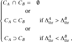 (3)
(3)
where  and
and  are the threshold used to form clusters A and B respectively. These are the only conditions needed to build a single-root tree structure. The whole set of clusters obtained by scanning over Δthr are nodes of a tree. Starting from C0 and ascending the tree (e.g. going in the direction of lowering Δthr) the formed clusters are characterized by a decreasing number of events, and by the property that the boundaries of a cluster Cj are contained within the boundaries of other clusters (ancestor clusters).
We can identify an ancestor and descendant hierarchy. Starting from a cluster CA, it can be identified as an ancestor if there exists at least one other cluster CB such that
 (4)
(4)
If such a condition is satisfied, CB is a descendant of CA; otherwise CA is a leaf of the tree. The ancestor of all the other clusters is C0. Due to Eq. (3), the total number of built clusters is ≤ N.
5 Coincidence cluster probability
There is a chance that reconstructed clusters does not represent a flaring period, but a statistical fluctuation over the true flux of the source. To estimate the probability of obtaining a cluster by chance, we consider as null hypothesis the case that the whole sample is uniformly distributed within the extraction interval (for the Fermi-LAT data sample this means the case that the background diffuse emission, background sources, and the foreground source give a steady contribution during the observing period within the extraction region R68 (typei, Ei)). Suppose we have N uniformly distributed events within the extraction interval. For the case of the Fermi-LAT data sample the extraction interval is the cumulative exposure domain (it must not be confused with the extraction region in aperture photometry). Let us assume without loss of generality that the extraction interval is the unitary extraction interval (0, 1]. Suppose we count the events within a window of fixed length (d) within the extraction length. Suppose also that the window is moved within the unitary extraction interval. Following the notation in Glaz et al. (1994), scan statistics evaluates the probability P{Nd > m} of finding more than m events within a moving window of length d (with d contained in the unitary extraction length), where Nd = sup{Nx,x+d;0 ≤ x < 1 − d}, and Nx,x+d is the number of events in the interval (x, x + d], 0 ≤ d < 1 (see Glaz et al. 1994, for a detailed explanation). In spite of the ease of the enunciation, statisticians took over 30 yr to find a solution for P{Nd > m} (Huntington & Naus 1975). The implementation of the solution is practically unfeasible and approximate solutions are often proposed (see e.g. Huffer & Lin 1997; Haiman & Preda 2009). To approach the problem we made use of the relation reported in Glaz et al. (1994),
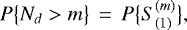 (5)
(5)
where P{ is the distribution of the smallest of the m-spacings. The m-spacings
  are defined by
 (6)
(6)
where {X(i)} is the ordered set of uniformly distributed events {Xi}, and  is the ordered set of m-spacings
  (see Glaz et al. 1994, and references therein for detailed definitions). The distribution of
  can be easily obtained with simulations. Tables were prepared with the cumulative distribution of
  for a uniform distribution of N points on a segment. The tables1 cover values of N from 3 up to 106. The tables are filled up running NR = 4 × 10⁶ random samples of N events extracted with a uniform distribution. The number of total random extractions is of the order of 1015 to fill all the tables. We used the Marsaglia-Zaman RANMAR random engine (Marsaglia et al. 1990; James 1990) contained in the Class Library for High Energy Physics (CLHEP), which has a very long recycling period of ~ 10144 and does not show correlated sequences of extracted variables (nearby generated points are not mapped into other sequences of nearby points).
Each table corresponds to a fixed sample size N*. Each row of a table contains the distribution for a fixed m-spacing. Each element of a row reports the length  of the m-spacing that corresponds to a certain probability
  . Columns are prepared for probabilities
  with t = 2, 2.5, 3, 3.5, 4, 4.5. The reported lengths of m-spacings have a statistical accuracy that corresponds to a relative accuracy on probability
  of 0.3%, 0.6%, 1.3%, 3.3%, 8.8%, 27% for t = 2, 2.5, 3, 3.5, 4, 4.5 respectively. For N ≤ 300, the tables for all the m-spacings and for all the sample sizes were filled.
Scan statistics cannot be applied directly to search for flaring period, because it makes use of a moving window of fixed length (d in the discussion above). The analyst must know the duration of the flare in advance to choose the value of d. Nagarwalla (1996), Glaz & Zhang (2006) and Cucala (2008) investigated the problem. In particular Glaz & Zhang (2006) and Cucala (2008) applied a scan-statistics approach iterated on a set of windows of different length. Once a set {Ci} of clusters is obtained, we want to investigate if they could or could not be considered random fluctuations from a uniform distribution extracted within the extraction interval. If the problem is limited to studying the sub-sample of {Ci}, which consists only of clusters of fixed size, the problem is univariate, and the m-spacing statistics can be applied directly (using Eq. (5) and the tables with the distribution of  ) to evaluate chance cluster probability, which is called here
  to underline that it is valid for the scan-statistic case). But the case we have to face is that the cluster size is not held fixed; the distribution of {Ci} is multivariate and
  does not correspond to chance cluster probability. In any case, we can report
  in Gaussian standard deviation units
  , where the information of Ci is all contained in the index i. From every Ci we evaluate
  . From the entire set {Ci} we obtain the set
  . We study the statistical distribution of
 (7)
(7)
where the maximum is evaluated over all the formed clusters. The variable Θ is called Maximum Scan Score Statistic (Glaz & Zhang 2006). The distribution of Θ is univariate and can be studied with simulations in the case of a uniform data set. For every simulated sample of size N, we apply the iSRS clustering procedure and we obtain {Ci} (and thence  ). From
  , we found Θ according to Eq. (7). From a set of simulated samples (with the same size N), the distribution of Θ is obtained.
We define a sample as false-positive when Θ is above a predefined value Θ*. The frequency of false-positive samples is fcoinc. It can be denoted with fcoinc(Θ*). The cumulative distribution of Θ is 1 − fcoinc(Θ*). The Monte Carlo results are reported in Fig. 1. We show the obtained fcoinc as a function of sample size N for a set of chosen Θ*. The curves reported in Fig. 1 show a change of slope for sample sizes below ~30. It is neither due to approximations on the distribution of  , nor to the interpolations for the m-spacings and for the sample sizes because for sample sizes below ~300, the tables for all the m-spacings and for all the sample sizes were filled.
The m-spacings tables were used to evaluate fcoinc. If a table for a given sample size has not been prepared, an interpolation using the tables with the nearest sample sizes is performed. If an m-spacing row for a certain sample size has not been prepared, an interpolation using the nearest m-spacings is performed. The systematic on false-positive frequency is due to the accuracy of the m-spacings tables and on the interpolations on sample size and on m-spacing. The statistical accuracy of m-spacing tables has been already discussed. Interpolation on sample size was found to introduce a systematic relative error of 10% on the evaluation of fcoinc. The interpolation on m-spacings introduces a systematic relative error of 7%, 2%, <1% for sample of size 105, 25 000, 1600 respectively. In the following, we refer to the probability distribution of Θ with PiSRS (tiSRS in standard Gaussian units) to underline that it is obtained without constraints on the cluster-size and using the iSRS clustering scheme.
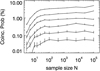 |
Fig. 1 Cluster coincidence probability prepared with a Monte Carlo for samples of N events. Curves refer to the frequency of false-positive samples obtained for different Θ* thresholds: from top to bottom Θ* = 2.75, 3, 3.25, 3.5, 3.75, 4. |
6 Removal of random clusters
We have prepared a set {Ci} from the original sample using the iSRS clustering. If the source was steady, the distribution of Θ prepared by applying Eq. (7) to the set {Ci} is known. We can choose a confidence level, and find the corresponding Θc.l.. If we have a uniformly distributed sample of size N, there is a probability coincident with the confidence level that
 (8)
(8)
If the source, instead, had a flare, the m-spacings are not distributed as in the case of a uniformly distributed sample. As a consequence, Θ also is not distributed as in the case of a uniformly distributed sample, and for a sub-set of clusters  , we could obtain values of
  . We will use Eq. (8) to test the hypothesis that the sample under investigation is uniformly distributed, and we call statistically relevant with respect to the whole investigated period the clusters of the sub-sample
  .
.
A special object is added as the first element of {Ci}. Its boundaries are the beginning and end of the observation. Its effective length ( ) is the whole extraction interval and its size (Nwhole) is the sample size N. We will denote it with Cwhole. It does not obey Eq. (2). It is the root.
The set {Ci} is ordered with respect to Δthr. The clusters of the ordered set {Ci} have to be considered as candidates. A discrimination procedure is applied in order to build a sub-set of clusters that describe the source variability within the investigated period. The removal procedure is applied to all the clusters starting from C0 and continues with the clusters with lower Δthr. As a first step, we have to evaluate if C0 needs to be considered as a random fluctuation from a uniformly distributed sample of size N and extracted within the whole period of investigation. If C0 belongs to the sub-set of statistically relevant clusters, it is maintained, otherwise it is removed from the original set. If C0 is maintained, the most conservative hypothesis is that the events within C0 are uniformly extracted within a period of length coincident with the effective length of C0. Going on with the removal procedure, for a certain index of the ordered list of candidate clusters, we found a cluster C*. We have to choose whether to accept or reject C*. We identify distinctively its direct accepted ancestor Cp (parent). Due to the fact that the removal procedure is ordered with respect to Δthr, Cp has already been accepted. The most conservative hypothesis (null hypothesis) is that the sample (of size Np) of the events contained in Cp is uniformly distributed within the effective length ( ) of Cp (e.g. that the source flux was steady during the period identified with Cp). If no parent cluster exists, the root (Cwhole) is considered as the parent instead, and Nwhole and
  are used. We accept C* if the null hypothesis is rejected according to the chosen confidence level. The removal decision of cluster C* follows the same arguments used for the removal decision of cluster C0, but instead of evaluating whether C* is a statistically relevant cluster with respect to the whole investigated period, we make the following evaluation: we consider only the reduced sample of events contained in Cp. This sample is of size Np and it is assumed to be of length
  . We evaluate whether C* is among the statistically relevant clusters for the reduced sample. We call these clusters statistically relevant with respect to the period described by the cluster Cp, or, more concisely: statistically relevant with respect to Cp. If C* is statistically relevant with respect to Cp, it is maintained, otherwise it is removed. If C* is maintained, the new conservative hypothesis is that C* describes a period of steady activity.
The statistical discrimination procedure is performed for all of the candidate clusters. The flowchart of the procedure is reported in Fig. 2. The surviving clusters have new properties:
- 1.
they are all statistically relevant with respect to their own parents;
- 2.
the events contained in any parent cluster do not belong to a uniform distribution.
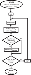 |
Fig. 2 Flowchart of the removal of random clusters. At beginning we have the ordered set {Ci} obtained with the iSRS clustering. The initial list of survived clusters |


7 Unbinned light curves
Two opposite scenarios are discussed: a steady and a flaring source. If the source was steady during the whole observing period, we expect no cluster to survive the removal of random clusters, apart from the root Cwhole. There is a chance probability of <1.3o (if the confidence level is set to 99.87%) of obtaining one or more clusters from a uniformly distributed sample.
It is useful to go over the iterated SRS clustering, and through the removal of random clusters for the case of a source that underwent a flare during the investigated period. The cluster property 2 states that clusters and chains of clusters are expected during activity periods (when the hypothesis of steady source is false). Once the set {Ci} is prepared, there could be at least one candidate son cluster C that is statistically relevant with respect to the whole observing period (if there are several relevant clusters, the one with the largest Δthr is chosen). In this case, the null hypothesis of a steady source is rejected and the new conservative hypothesis is that C
 corresponds to a period of flat activity. Continuing the removal of random cluster procedure, we might find at least one cluster C
 (descendant of an accepted cluster Ci) that is statistically relevant with respect to the period identified with Ci (if there are several relevant clusters, the one with the largest Δthr is chosen). We reject the hypothesis of a steady source within the period identified with Ci, and maintain the cluster
  . The new conservative hypothesis is that the cluster
  identifies a period of flat activity. The procedure stops when no son clusters exist for which the new conservative hypothesis can be statistically rejected. Clusters with no sons identify the flare peaks: the leaves of the tree are found when the flare peak is found (the light curve at its peak is locally flat or the paucity of collected photons prevents the procedure from continuing). The set C
 ,C
,C , C
, C ,…, C
,…, C , C
, C is the chain describing the flaring period. The cluster C
 is a leaf of the tree. It represents the activity peak. Property 1 states that each cluster of the chain is statistically relevant with respect to its parent: the chain of clusters is a statistically filtered representation of the flaring period. Examples of real unbinned light curves are reported in Figs. 7 and 8. Each horizontal segment represents a cluster of the tree: it subtends the temporal interval characterizing the cluster. Its length is the effective length of the cluster in the temporal domain; its height is the mean photometric flux of the source within the subtended temporal interval. Each reported cluster cannot be considered a random fluctuation (according to the chosen c.l.) from a flat activity period identified by its parent cluster. The unbinned light curve as a whole is a representation of the tree hierarchy. The peaks of flare activity are the clusters with no associated sons. This means that within each identified period of activity peak, we did not found any statistically relevant sub-set of events describing a period of larger flux. The identification of the activity peaks is a direct result of the unbinned light-curve procedure. The reported clusters are not independent. Equations (3) and (4) state that clusters describing the same flare are all correlated, because their intersection is not the empty set. Therefore, the evaluation of the temporal full width half maximum (FWHM) of reconstructed flares can be performed starting from the unbinned light curve, but the statistical uncertainty of the temporal FWHM must be evaluated using simulations.
8 Performance of the method for the Fermi-LAT: flare detection efficiency, flare reconstruction capability
We tested the proposed procedure with simulations. As far as gamma-ray background varies with celestial coordinates, and chance detection probability depends on source mean flux and background, the performance of the method depends on the investigated source. We focus here to the case of a flat spectrum radio quasar (FSRQ): 3C 454.3. The extraction region is centred on the coordinates of the source and its radius corresponds to the containment of 68% of photons from the source. Background level corresponds to the observed background for the source (in Appendix D we will show the method to evaluate background). We computed the Fermi-LAT exposure for 3C 454.3 with a bin size of 86.4 s from the beginning of Fermi-LAT scientific operations, till 2015 November 16 (see Appendix C for the details of exposure preparation). we simulated ideal flares photon by photon with a temporal shape
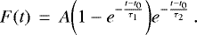 (9)
(9)
In order to reduce the total number of simulation runs, we chose τ1 = τ2 = τ. Coefficients A and τ are chosen to simulate flares with a given peak flux and temporal FWHM. Ideal flares are simulated assuming a flat exposure. We used the computed exposure to accept or reject simulated photons from the source and from background. The accepted photons are the final photon list. The chosen threshold probability  is 99.87% (e.g.
  = 3).
= 3).
In Fig. 3 we report the detection efficiency for flares with a temporal FWHM of 0.01, 0.1, 1, 10, and 100 days, and with peak flux from 10−8 to 10−5 ph cm−2 s−1 (E > 0.3 GeV). For flares with a FWHM above one day (slow flares), the detection efficiency rises fast around the threshold flux. On the contrary, below one day (fast flares), it rises slowly, because the Fermi-LAT observes sources for windows of 10–20 min each orbit or two (and sometimes four). Extremely fast and bright flares can be detected, even if their peak emission lies outside the observing windows, provided that the sampled tails of those flares are bright enough to be detected. The flux F50% (F20%) corresponding to a detection efficiency of 50% (20%) is reported in Fig. 4 as a function of temporal FWHM of the simulated flares. Two cases are reported, corresponding to faint (NSRC ≤ 0.2NBKG) and bright sources (NSRC ~ 16NBKG), where NSRC and NBKG correspond to the total source and background counts integrated in 7.25 yr with Fermi-LAT collected in the chosen extraction region. Below 0.01 d, the computed values of F20% are very similar for bright and faint sources, because flares could be detected provided they happened outside the exposure gaps. The satellite pointing strategy affects the detection efficiency and dominates over statistic.
The peak flux reconstruction capability is reported in Fig. 5. For bright flares the reconstructed flux (Frec) approaches Fpeak. In the region where the detection efficiency (see Fig. 3) is larger than  , the reconstructed flux (Frec) is in the range Fpeak∕2 < Frec ≤ Fpeak. The ratio Frec /Fpeak increases while Fpeak increases. For the brightest flares Frec approaches Fpeak. The lowering of Frec /Fpeak for faint flares is due to the fact that for faint flares, the activity peak is not well resolved. In the region where the detection efficiency is smaller than
  , the ratio Frec /Fpeak increases while the Fpeak decreases, and it is lower than two. For flares shorter than 1 d, the reconstructed flux shows large deviations from the simulated one, because of the Fermi-LAT observing strategy (for the majority of the flaresthe peak flux is not sampled at all). For flares of FWHM = 0.01 d, on average the ratio Frec /Fpeak decreases while Fpeak increases. The reason is that faint flares are preferentially detected when the peak of emission is sampled.
Temporal FWHM is estimated starting from the unbinned light curves. It is derived assuming that the underlying flare has a pyramidal shape. The temporal FWHM reconstruction capability is reported in Fig. 6. For flares with temporal FWHM larger than 1 d, the reconstruction capability is poor for faint flares, and the reconstructed FWHM exceeds the simulated FWHM. The FWHM of flares with simulated FWHM shorter than 1 d cannot be reconstructed, due to the temporal gaps of the exposure.
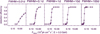 |
Fig. 3 Detection efficiency for flares with FWHM of 0.01, 0.1, 1, 10, 100 d as a function of the simulated flare peak flux. The observing period is 7.25 yr. |
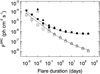 |
Fig. 4 Peak flux detection threshold as a function of the simulated flare duration, reported as FWHM. Triangles (squares): flux threshold is defined as the peak flux for which half (20%) of the simulated flares are detected. The observing period is 7.25 yr, E > 0.3 GeV. The extraction radius corresponds to the containment radius for 68% of events. Open squares and triangles refers to a faint source (giving a total number of counts on Fermi-LAT that is 20% of the background counts within the scrutinized period). Filled symbols refer to a bright source (corresponding to the case of 3C 454.3). Curves refer to sensitivities calculated assuming constant exposure, hat shaped flares, for
|

9 Results for some gamma-ray samples and conclusion
Extensive results for an astrophysical problem will be shown in a forthcoming paper. To explain the advantages and drawbacks of the method, we report some cases here (details about data preparations are in Appendix C). McConville et al. (2011) studied the activity of the FSRQ 4C +55.17 from 2008 August to 2010 March. They found no evidence for gamma-ray variability within the scrutinized period. The authors also found energy emission up to 145 GeV (observer frame). Their multi-wavelength investigation shows the source is compatible with a young radio source, with weak or absent variability. The unbinned photometric light curve of the source for a period of 7.25 yr of monitoring in gamma ray with Fermi-LAT does not show flaring activity in the range 0.3–500 GeV with a confidence level of 99.87%.
We show here the unbinned photometric light curves for the Crab Nebula in the energy range 0.1–500 GeV (Fig. 7) and for the FSRQ 3C 454.3 (Fig. 8) in the energy range 0.3–500 GeV.
These sources are among the brightest gamma-ray sources in the sky, and the unbinned light curves are fully representative of source variability. For both the sources we used Ntol = 50 to reduce fragmentation. In Figs. 7 and 8 background is not subtracted, but it is negligible. Each horizontal line represents a survived cluster. The length of the cluster (in temporal domain) is the length of the segment; the density of the cluster is the flux level of the segment. Flux level includes background sources and diffuse background emission). The ground level is the mean source flux (+background) over the whole scrutinized period. Each horizontal segment is statistically relevant above the father one according to the chosen confidence level.
The Crab Nebula’s large variability in gamma rays was first observed with AGILE (Pittori et al. 2009; Tavani et al. 2011). Pittori et al. (2009) and Tavani et al. (2011) argue the variability is due to a component with a cut-off around 0.5 GeV, so we report here the unbinned light curve obtained for confidence levels of 99.87%, in the energy range 0.1–500 GeV. In the low energy band the instrumental PSF of the Fermi-LAT is large, but the Crab flux is extremely bright and contamination from nearby sources can be neglected. The unbinned photometric light curves reported here refer to the Fermi-LAT observing period only. Due to the complex unbinned light curve of the Crab Nebula, we report in Fig. 7 two periods only, referring to the flaring period investigated in Striani et al. (2013) and in Abdo et al. (2011a) (left panel) and the one investigated in Buehler et al. (2012; right panel). A comparison between the unbinned light curve proposed here and previous works is useful to show the strength and weakness of the proposed method. The top panel in Fig. 7 shows a flare that is not well resolved in Abdo et al. (2011a). The same flare is reported also as F7 in Striani et al. (2013). We obtain a peak photometric flux on MJD 55459.793. The temporal FWHM estimated from the unbinned light curve reported here is 0.23± 0.12 d (the error is evaluated from the Monte Carlo simulations reported in Fig. 6). The temporal FWHM could be overestimated by a factor of ~2. The unbinned light curve analysis shows that it is the shortest flare ever reported for the source so far. The feature F6 in Striani et al. (2013) is not detected with the unbinned light curve, but in the approach proposed here, clusters with low statistical significance are disregarded.
The other panel in Fig. 7 can be compared to a finely segmented light curve produced with likelihood analysis in Buehler et al. (2012). Those authors prepared a fixed exposure light curve (the binning is variable in time, the mean bin duration is 9′). The analysis in Buehler et al. (2012) makes use of the Bayesian Block procedure for binned data to statistically evaluate variability, and performs an exponential fitting of the rising part of the two resolved flares. The method proposed in this paper reveals the same two flares, centred on MJD 55665.110 and MJD 55667.319, with temporal FWHM of 1.2 ± 0.4 and 1.1 ± 0.4 d respectively, in agreement with the results reported in Buehler et al. (2012).
Flares from the FSRQ 3C 454.3 are intensively studied. The binned light curve for the first three years of Fermi-LAT observations of 3C 454.3 is reported in Abdo et al. (2011b) with a time bin of one day. The light curve for the first 5.1 yr of Fermi-LAT observations is reported in Pacciani et al. (2014) with a time bin of four days (E > 0.3 GeV). The light curve for the following one year of the source is reported in Britto et al. (2016) with a one day time bin. A shorter period of activity is reported with a 3 hr time bin in Coogan et al. (2016) and in Britto et al. (2016). The procedure proposed here detects the flares of the source with some exceptions. It does not detect the secondary flare around MJD 55330 shown in the 0.1–500 GeV light curve reported in Abdo et al. (2011b). Integrating data in the energy range 0.1–500 GeV, the secondary flare is detected with a confidence level of 97.7%.
In Abdo et al. (2011b), the authors report a flare fine structure during the brightest activity period of the source (around MJD 55 517–55 520) and they investigated the fine structure fitting a model of four flares to the data in the 0.1–500 GeV energy range. The method proposed here reveals a single flare in the energy range 0.3–500 GeV (with 99.87% c.l.), without making assumptions on flare shape. Sub-structures emerge integrating data in the 0.1–500 GeV (97.7% c.l.). In conclusion, for the brightest flares, the study of fine structure making use of a fitting strategy, is the preferred method, that has to be statistically compared with the null hypothesis of a single flare.
The unbinned photometric light curves shown here for the Crab Nebula (Fig. 7) and for the FSRQ 3C 454.3 (Fig. 8) show both the advantages of the procedure and the remaining drawbacks. The peak flux activity period is resolved only when it is larger than the mean flux (including diffuse background and nearby sources). Weak flares from faint sources, surrounded by bright sources, cannot be resolved. This is the case for 3C 345, whose flaring activity (see e.g. Reyes & Cheung 2009) is washed out by the presence of the nearby bright sources 4C 38.41, Mkn 501, and NRAO 512 at 2.2°, 2.1°, and 0.48° from the foreground source respectively. Isolated flares are resolved according to sensitivity limit. As far as there is no time binning, there are no time-bin related issues. The detection of fast flares from the Crab Nebula, and large temporal structures as in the case of 3C 454.3, is obtained without ad-hoc assumptions or peculiar choices in the analysis. There is, however, a resolving-power drawback. In fact there is the need to define Ntol to avoid fragmentation. The consequence is that consecutive flares, whose peak activity is separated by less than 2Ntol gamma rays, could be merged together, as discussed in Appendix B; merging involves faint flares.
A fraction of fast and bright flares can be detected depending on the pointing strategy of the Fermi satellite. We evaluated that Fermi-LAT can detect flares with a temporal FWHM as short as 10–20 min and peak flux ~10−5ph cm−2 s−1 (E > 0.3 GeV) with a detection efficiency of 20% (at 99.87% c.l.). But this evaluation depends on the temporal profile of the flare. It is difficult, indeed, to evaluate the peak flux and temporal FWHM of bright flares with typical timescales less than 0.1–0.3 d.
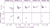 |
Fig. 5 Peak flux reconstruction capability. Top panels: mean (open diamonds) and standard deviation (vertical lines) of the reconstructed flux (normalized to the simulated peak flux) are reported as a function of the peak flux for different values of the FWHM. Bottom panels: number of flares (normalized to the number of detected flares) for which the reconstructed peak flux is below a factor of
|

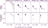 |
Fig. 6 Temporal FWHM reconstruction capability. Top panels: mean (open diamonds) and standard deviation (vertical lines) of the reconstructed FWHM (normalized to the simulated FWHM) as a function of the peak flux for different values of the FWHM. Bottom panels: number of flares (normalized to the number of detected flares) for which the reconstructed temporal FWHM is below a factor of
|

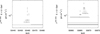 |
Fig. 7 Unbinned light curve for the Crab Nebula, obtained with Ntol = 50, E > 0.1 GeV, extraction radius corresponding to the containment of 68% of photons from the source. Confidence level is 99.87%. The unbinned light curve is produced for 7.25 yr, but only two already studied periods are shown for a direct comparison of the results: left panel reports the observing period investigated in Striani et al. (2013) and in Abdo et al. (2011a). Right panel reports the observing period investigated in Buehler et al. (2012). Each horizontal segment represents a cluster: it subtends the temporal interval characterizing the cluster; its length is the length of the cluster in the temporal domain; its height is the mean photometric flux of the source within the subtended temporal interval. The unbinned light curve as a whole is a representation of a single-root tree like hierarchy. The bottom segment is the root cluster. Ascending the tree corresponds to go from the bottom up of the plotted diagram of clusters. For each cluster, a parent can be identified (the boundaries of a son cluster are within the boundaries of the parent). All the reported clusters which can be regarded as parents do not describe flat activity periods (the hypothesis that the events within a parent cluster are uniformly distributed is rejected with a confidence level of 99.87%). Clusters and chain of clusters are expected for flaring periods, when the hypothesis of uniformly distributed events is false. Leaves are the activity peaks. Every son cluster is statistically relevant with respect to its parent, according to the chosen confidence level. Therefore the unbinned light curve is a statistically filtered representation of the source activity. |
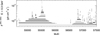 |
Fig. 8 Unbinned light curve for the FSRQ 3C 454.3, obtained with Ntol = 50, E > 0.3 GeV, extraction radius corresponding to the containment of 68% of photons from the source, 99.87% c.l. See caption of Fig. 7 for an explanation of the diagram for the unbinned light curve. |
10 Discussion
We have developed a procedure to identify activity peaks in time-tagged data. We applied the proposed procedure to gamma-ray data only, but it can be applied to any time-tagged data set, or more in general to any ordered set of uniformly distributed events. The basic task of the procedure is the identification of statistically relevant periods within a supposedly uniformly distributed sample. There are no fittings in the procedure, hence no fitting-related convergence issue. We have shown with simulations and with real data that the procedure is capable of detecting activity peaks without any prior knowledge of their shape and temporal size.
There is a parameter in the procedure (Ntol) introduced to face with fragmentation artefact. We have shown how to choose it and the drawback arising with its introduction. Small samples (of 103 events or less) can be statistically investigated to search for variability setting Ntol to one for these samples.
Knowledge of the performance and limitations of a method are crucial for applying it to any astrophysical case. We explored the limitation of the procedure. We also investigated sensitivity limits and the performance of the method for a specific case. The procedure isbased on scan statistics and on extensive Monte Carlo simulations. The results of simulations are for a general use and are contained in short tables for the statistics of m-spacings and for the frequency of false-positive samples. Even if it is conceivable to extend the tables to extremely large samples, the introduction of asymptotic scaling laws could be appropriate to overcome large computational effort. A step towards this is performed in Prahl (1999). The author developed a Poisson test based on a semi-analytical method. The test is based on the distance between contiguous events (e.g. on the m-spacing problem, with m = 1). The extension of that semi-analytical method to m > 1 is indeed mandatory to explore the full spectrum of variability for extremely large samples. Other approaches to obtain asymptotic solutions to the problem are investigated for example in Huffer (1997) and in Boutsikas et al. (2009). The computational effort to produce unbinned light curves from an ordered set of N events is extremely low (once the chance cluster probabilities are all tabulated). The procedure that produces clusters evaluates no more than Ntol × N distances between events. For all the examples reported, the iteration on Δthr spans no more than five decades with 20 steps per decade. The total number of evaluated distances is therefore no more than 100 × Ntol × N. The total number of clusters is no more than N, because the intersection of two clusters coincides with the smallest of them or it is the Empty Set. As far as chance cluster probabilities are all tabulated, no more than N probabilities are extracted from the tables.
Acknowledgements
I am grateful to I. Donnarumma and A. Stamerra for discussions, and to the anonymous referee for comments. L.P. acknowledges contributions from the grant INAF SKA-CTA.
Appendix A Fragmentation artefact and the choice of the Ntol parameter
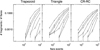 |
Fig. A.1 Frequency of Fragmentation artifact as a function of the events collected during the flaring period. The three panels are for the following temporal shapes: trapezoidal (left panel), triangular (central panel), temporal shape described in Eq. (9) (right panel). The clustering scheme of Eq. (2) is used. Continuous lines are used to connect the evaluated frequencies for the same tolerance parameter. Dashed lines are used to connect evaluated frequency to upper limits (99.87% c.l.). From top to bottom curves, tolerance parameters is set to 1, 3, 5, 10, 25, 50, 100. |
In the proposed procedure, fragmentation is an artefact introduced with clustering. In the case of a period of flat source activity (with flux Fflat), the analyst expects to find a single cluster describing the flat period. The construction of clusters making use of Eq. (1) leads to the subdivision of the flat period into several clusters. We call fragmentation this artefact. In fact, for Δthr ~ 1∕Fflat, we expect half of the exposure spacings among contiguous events to be larger than 1∕Fflat. The result is the construction of several clusters during the flat period. Fragmentation is not limited to periods of flat activity, but can occur also for flaring periods. If we have a flare, once we have chosen a value for Δthr, we expect to build a single cluster, but, due to the stochastic nature of the problem, several clusters can form. The clustering scheme obeying Eq. (2) reduces the occurrence of fragmentation provided that a suitable Ntol parameter is chosen. The evaluation of the occurrence of fragmentation is performed here with simulations, testing the proposed algorithm with three test-functions: trapezoidal, triangular, or the temporal shape described by Eq. (9). Background and steady source activity is neglected. For the case of trapezoidal shape, 80% of events are simulated within the flat period (the superior base of the trapezoid). We consider the cases that the instrument collects 400, 1600, 6400, 25 × 103, and 105 photons during the activity period under examination. For each temporal shape, and each photon statistic, we run up to 3 × 10⁴ simulations. Peaks are identified following the procedure proposed in this paper. The tolerance parameter is set to 1, 3, 5, 10, 25, 50, and 100. Fragmentation appears if there is more than one detected peak for a simulated activity period (e.g. for a simulation). Results are shown in Fig. A.1. A tolerance parameter of 50 is suitable for flares with up to 25 × 103 events: with this choice, fragmentation occurrence is at the level of 1% or less. Moreover this value is useful to describe a large activity plateau with 105 events. For flaring periods of 103 events or less, a tolerance parameter of 1 could be chosen. The following procedure is suggested to correctly choose the Ntol parameter. Obviously, the probability of fragmentation rises with the number of flare events, and it decreases with increasing Ntol. If we could know the number of events (Nf) of the activity periods, we could evaluate the fragmentation probability at a given Ntol and at the number of flare events corresponding to Nf for the worst case among the three test functions reported in Fig. A.1. Then we could choose an Ntol that keeps fragmentation probability at the desired level. Before data analysis is performed, we do not know the number of events of each flare, but the total sample size is known. If the sample size is 103 events or less, the tolerance parameter can be set to Ntol = 1. This choice allows for the fragmentation artefact to be below 1% for each detected flare (from the worst case among the ones reported in Fig. A.1 for Ntol = 1). For larger sample sizes, the suggested procedure is to prepare a preliminary unbinned light curve with the tolerance parameter set to a large value (e.g. Ntol = 100). From the set {Ci} of clusters surviving the removal procedure, each son of the root contains all the events of one or more flares, and they are the clusters with the largest size. The analyst must choose the accepted cluster with the largest size (excluding the root). The number of events of this cluster (Nmax) is equal to or larger than the number of the events of the brightest flare. The value of Nmax can be used together with the fragmentation estimates reported in Fig. A.1 to choose the correct value for Ntol in order to maintain the fragmentation probability below a predefined level for each flaring period. The obtained value of Ntol can be used to produce the final unbinned light curve. As an example, if the analyst finds from the preliminaryunbinned light curve that the cluster with the largest size (excluding the root) contains 25 × 103 events, from the three test functions reported in Fig. A.1, he obtains that Ntol = 50 gives a fragmentation probability of ~ 0.7% for the worst case (triangular shape flare). Therefore, if a fragmentation probability of ~ 0.7% is considered acceptable by the analyst, the final unbinned light curve can be prepared with Ntol = 50.
Appendix B Multiple flares resolving power
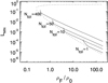 |
Fig. B.1 Resolving power capability for various Ntol parameters. Computation refers to two identical box-shaped flares: L is the width of each flare, ρF is the event density of the flare, and ρ0 is the background event density. There are Ntol background events in between the two flares. The continuous curves represent the minimum flare width for which the two contiguous flares are resolved. The dotted curve is the sensitivity limit (99.87% c.l.) for two identical box-shaped flares. For any given
|

The proposed clustering scheme (Eq. (2)) avoids the fragmentation artefact, provided that a suitable Ntol parameter is chosen. If two contiguous flares are separated by more than 2Ntol events, the SRS clustering scheme does not merge them. If two contiguous flares are separated by no more than 2Ntol events, they could be glued together and a resolving power issue can arise: flares are described by a chain of clusters. The two flares are roughly resolved if for each flare there exists at least a statistically relevant cluster (the cluster with the shortest Δthr) for which Eq. (2) is not satisfied. In Fig. B.1 we show the results of such an evaluation assuming 4700 background events uniformly distributed on a unitary segment. This background level corresponds to the background counts within a circular region of radius R68 (typei, Ei) around the FSRQ 3C 454.3 (see Appendix D). The gluing effect is evaluated for two identical box-shaped flares. The width of each box is denoted with L, the event density of the flare (the flare flux) is denoted with ρF, and the background event density is denoted with ρ0. We assumed the case in which there are Ntol events in between the two box-shaped flares (for a number of events larger than 2Ntol in between the two flares, there is no gluing). The glued cluster can have no more than 3Ntol + 2(ρF + ρ0)L events, and have a size  . We denote this cluster as Cglued and ρglued the mean event density of the glued cluster. We evaluated the minimum flare width (Lmin) for which clusters of length L and (ρF + ρ0)L events are statistically relevant at 99.87% c.l. with respect to Cglued. The minimum L is reported in Fig. B.1 as a function of
  . For comparison, we report in Fig. B.1 also the sensitivity limit for two identical box-shaped flares. For a single flare, the sensitivity limit has a horizontal asymptote at L = 1. For two identical flares (such as in the present case), the horizontal asymptote is at L = 1∕2 (top sensitivity limit curve). For any given
  , two identical flares are resolved until their width is larger than Lmin. In the interval between Lmin and the bottom sensitivity limit, the flares are detected as a single flare. There is a range of values of
  for which Lmin is not defined. Within this range, the two identical flares are always resolved, if they are detectable above background. The lower Ntol is set, the lower is the gluing. The case Ntol = 1 corresponds to the simple clustering of Eq. (1).
Appendix C Fermi-LAT data preparation
We performed data preparation and likelihood analysis tasks using the standard Fermi Science Tools (v10r0p5), the PASS8 Response Functions (P8R2_SOURCE_V6), and standard analysis cuts. The gtselect task was used to select SOURCE class events (evclass = 128), collected within 20° from the investigated source. Earth limb gamma rays were rejected applying a zenith angle cut of 90°. To prepare input files to the likelihood procedure, only good-quality data, taken during standard data taking mode, were selected using the gtmktime task. Livetime cube was prepared taking into account the zenith angle cut. Exposure maps were prepared using standard recipes. Unbinned likelihood analysis was performed including all the sources from the third Fermi-LAT catalogue (Acero et al. 2015) within the chosen region of interest (ROI). For the investigated source and for sources within 10° from the ROI centre, all the spectral parameters were allowed to vary. For all the other sources, only the normalization factor was allowed to vary.
To prepare input files to the gtexposure and to the SRS clustering procedure, good time intervals (GTIs) were prepared with gtmktime task for good-quality data, taken during standard data taking mode, and for source events outside the Earth’s limb. The finely binned exposure with a binsize of 86.4 s was prepared with the standard gtexposure tool, using the third Fermi Large Area Telescope source catalog (3FGL) catalogue spectral template for the investigated source. The filtered photon list is sorted with respectto time. The finely binned exposure and the filtered photon-list are the inputs of the algorithm described in this paper.
Appendix D Background level estimate
We evaluated the gamma-ray background level for 3C 454.3 using two methods.
First method: Between MJD 55 800 and MJD 56 100, the FSRQ 3C 454.3 underwent a period of extremely faint activity (see light curve in Pacciani et al. 2014). The unbinned likelihood analysis performed above 0.3 GeV with a region of interest (ROI) of 20° for that period gives a source flux of (0.75 ± 0.13) 10−8 ph cm−2 s−1, 184 source events collected by the Fermi-LAT (Npred), and a source test statistics (ts) of 79. The exposure to the source (evaluated using gtexposure) for that period is 2.5 × 1010 cm2 s (E > 0.3 GeV). There are 704 gamma-ray events collected above 0.3 GeV within R68(typei, Ei) (defined in Sect. 3) for the studied faint activity period. So we can assume 579 ± 45 background gamma rays within R68 (typei, Ei). The Fermi-LAT exposure to the source for the 7.25 yr period is 2.2 × 1011 cm2 s (E > 0.3 GeV). The extrapolated background for the whole period is 5200 ± 400 counts.
Second method (multiple background regions method): Background counts can be evaluated using a photometric method, using a suitable extraction region. But the background level varies with galactic coordinates, so we chose to extract background counts from 36 circular background regions. The centres of the circles are placed on a circumference of radius Rc = 10° centred on the position of the investigated source (3C 454.3). They are equally spaced on that circumference. The radius of circular background regions is dynamically chosen with the same criteria used for the definition of R68 (typei, Ei), but rescaled by a factor frescale = 4 with respect to R68(typei, Ei). For each background circular region, we can identify another background region, which is located in the opposite direction in the reference frame centred on the investigated source. We refer to these two as homologous regions. The exposure of each circular background region differs from the other regions and from the exposure of the investigated source. The sky scanning strategy of the Fermi satellite mitigates differences. Moreover, the choice of multiple background regions further reduces differences in the effective area between the source region and the mean of the surrounding background regions. The use of homologous regions cancels out the differences. The preparation of Fermi-LAT data for the SRS clustering handles Earth occultation, and discriminates Earth-albedo gamma rays using zenith angle cuts in gtselect (see Cicerone web pages2). The gtmktime procedure is used to prepare GTIs to account for the occultation of the source region only. The satellite is in near equatorial orbit, therefore the Earth albedo and Earth occultation GTIs mainly depend on the celestial declination of each region. There are periods in which the background regions are not occulted by the Earth but are removed from the analysis with gtmktime (this fact gives no systematic in the evaluation of background). Conversely, there are periods in which the background regions are occulted by the Earth (or collect Earth-albedo gamma rays) and the Earth-albedo gamma rays are filtered out with the gtselect procedure, but this filtering is not accounted for with gtmktime (gtmktime is used to prepare the GTIs to filter-out periods for which the source is below the Earth limb). This fact is not taken into account in the background evaluation procedure. It gives a systematic in the evaluation of background. There are two extreme cases. The first is for background regions located at the same celestial declination of the source, and 10° apart in right ascension. For such background regions, the reduction of background counts is a factor  . The detailed semi-analytical calculation, taking into account the satellite path along the Earth, shows that the average loss of background events (not accounted for in the built GTIs and in the exposure calculation) is ~ 1.7%. The second case is for regions at the same right ascension of the source, and when the source is at the edge of the Earth limb. In such a situation, there is a loss of background counts for the regions at the lower declination that is not accounted for by the exposure. The detailed calculation shows that the largest loss of events among regions is 22%, but the loss of counts involves less than half of the background regions. The average loss of background counts is 8.6%. For the purpose of this paper, we disregard these systematics. With this approximation and in the ideal case of no contaminating sources giving counts within the circular background regions, the background estimated performing the average of two homologous regions is a linear interpolation of the background level at the position of the investigated source. In order to remove contaminating sources, the three regions with the largest counts and their homologous are neglected. Moreover, the three regions with the shortest counts and their homologous are neglected. The background level at the position of the investigated source is estimated as the average from the counts of the surviving background circular regions (rescaled by a factor
  ). Using this method, the background counts within a region of radius R68(typei, Ei) centred at the position of 3C 454.3, during the extremely faint activity period, are 540 ± 30. This estimate is comparable with the first method. The extrapolated background for the 7.25 yr period is 4880 ± 270 counts. Using the multiple background regions method for the 7.25 yr period, the background level within a region of radius R68 (typei, Ei) centred on the position of 3C 454.3 is 4680 ± 80. The method of multiple background regions cannot be used for sources too close to the galactic plane, because in this case the average of the counts within the background regions is not representative of the background at the position of the investigated source.
References
- Abdo, A. A., Ackermann, M., Ajello, M., et al. 2011a, Science, 331, 739 [NASA ADS] [CrossRef] [PubMed] [Google Scholar]
- Abdo, A. A., Ackermann, M., Ajello, M., et al. 2011b, ApJ, 733, L26 [NASA ADS] [CrossRef] [Google Scholar]
- Acero, F., Ackermann, M., Ajello, M., et al. 2015, ApJS, 218, 23 [Google Scholar]
- Ackermann, M., Ajello, M., Albert, A., et al. 2013, ApJ, 771, 57 [NASA ADS] [CrossRef] [Google Scholar]
- Atwood, W. B., Abdo, A. A., Ackermann, M., et al. 2009, ApJ, 697, 1071 [NASA ADS] [CrossRef] [Google Scholar]
- Boutsikas, M. V., Koutras, M. V., & Milienos, F. S. 2009, in Scan Statistics - Methods and Applications, eds. J. Glaz, V. Pozdnyakov, & S. Wallenstein (Boston: Birkhäuser), 55 [Google Scholar]
- Britto, R. J., Bottacini, E., Lott, B., Razzaque, S., & Buson, S. 2016, ApJ, 830, 162 [NASA ADS] [CrossRef] [Google Scholar]
- Buehler, R., Scargle, J. D., Blandford, R. D., et al. 2012, ApJ, 749, 26 [NASA ADS] [CrossRef] [Google Scholar]
- Bulgarelli, A., Tavani, M., Chen, A. W., et al. 2012, A&A, 538, A63 [NASA ADS] [CrossRef] [EDP Sciences] [Google Scholar]
- Coogan, R. T., Brown, A. M., & Chadwick, P. M. 2016, MNRAS, 458, 354 [NASA ADS] [CrossRef] [Google Scholar]
- Cucala, L. 2008, Biom. J., 50, 299 [CrossRef] [Google Scholar]
- Glaz, J., & Zhang, Z. 2006, Stat. Probab. Lett., 76, 1316 [CrossRef] [Google Scholar]
- Glaz, J., Naus, J., Roos, M., & Wallenstein, S. 1994, J. Appl. Probab., 31, 271 [CrossRef] [Google Scholar]
- Haiman, G., & Preda, C. 2009, in Scan Statistics - Methods and Applications, eds. J. Glaz, V. Pozdnyakov, & S. Wallenstein (Boston: Birkhäuser), 179 [Google Scholar]
- Huffer, F. 1997, J. Am. Stat. Assoc., 92, 1466 [CrossRef] [Google Scholar]
- Huffer, F., & Lin, C. T. 1997, J. Am. Stat. Assoc., 92, 1466 [CrossRef] [Google Scholar]
- Huntington, R. J., & Naus, J. 1975, Ann. Probab., 3, 894 [CrossRef] [Google Scholar]
- James, F. 1990, Comput. Phys. Commun., 60, 329 [NASA ADS] [CrossRef] [Google Scholar]
- Lott, B., Escande, L., Larsson, S., & Ballet, J. 2012, A&A, 544, A6 [NASA ADS] [CrossRef] [EDP Sciences] [Google Scholar]
- Marsaglia, G., Zaman, A., & Tsang, W. W. 1990, Stat. Prob. Lett., 9, 35 [CrossRef] [Google Scholar]
- Mattox, J. R., Bertsch, D. L., Chiang, J., et al. 1996, ApJ, 461, 396 [NASA ADS] [CrossRef] [Google Scholar]
- McConville, W. F., Ostorero, L., Moderski, R., et al. 2011, ApJ, 738, 148 [NASA ADS] [CrossRef] [Google Scholar]
- Nagarwalla, N. 1996, Stat. Med., 15, 845 [CrossRef] [Google Scholar]
- Nauss, J. I. 1965, J. Am. Statist. Assoc., 60, 532 [CrossRef] [Google Scholar]
- Nauss, J. I. 1966, Technometrics, 8, 493 [Google Scholar]
- Pacciani, L., Tavecchio, F., Donnarumma, I., et al. 2014, ApJ, 790, 45 [NASA ADS] [CrossRef] [Google Scholar]
- Pittori, C., Verrecchia, F., Chen, A., et al. 2009, A&A, 506, 1563 [NASA ADS] [CrossRef] [EDP Sciences] [Google Scholar]
- Prahl, J. 1999, A&AS, submitted [arXiv:astro-ph/9909399] [Google Scholar]
- Reyes, L. C., & Cheung, C. C. 2009, ATel, 2226 [Google Scholar]
- Scargle, J. D. 1998, ApJ, 504, 405 [NASA ADS] [CrossRef] [Google Scholar]
- Scargle, J. D., Norris, J. P., Jackson, B., & Chiang, J. 2013, ApJ, 764, 167 [NASA ADS] [CrossRef] [Google Scholar]
- Striani, E., Tavani, M., Vittorini, V., et al. 2013, ApJ, 765, 52 [NASA ADS] [CrossRef] [Google Scholar]
- Tavani, M., Barbiellini, G., Argan, A., et al. 2009, A&A, 502, 995 [NASA ADS] [CrossRef] [EDP Sciences] [Google Scholar]
- Tavani, M., Bulgarelli, A., Vittorini, V., et al. 2011, Science, 331, 736 [NASA ADS] [CrossRef] [PubMed] [Google Scholar]
- Wallenstein, S. 2009, in Scan Statistics - Methods and Applications, eds. J. Glaz, V. Pozdnyakov, & S. Wallenstein (Boston: Birkhäuser), 2 [Google Scholar]
The tables are available in electronic form at the CDS.
https://fermi.gsfc.nasa.gov/ssc/data/analysis/documentation/Cicerone/Cicerone_Likelihood/Exposure.html (section: Excluding Atmospheric Background Events); https://fermi.gsfc.nasa.gov/ssc/data/analysis/scitools/aperture_photometry.html; https://fermi.gsfc.nasa.gov/ssc/data/analysis/scitools/data_preparation.html
All Figures
|
Fig. 1 Cluster coincidence probability prepared with a Monte Carlo for samples of N events. Curves refer to the frequency of false-positive samples obtained for different Θ* thresholds: from top to bottom Θ* = 2.75, 3, 3.25, 3.5, 3.75, 4. |
| In the text | |
|
Fig. 2 Flowchart of the removal of random clusters. At beginning we have the ordered set {Ci} obtained with the iSRS clustering. The initial list of survived clusters |
| In the text | |
|
Fig. 3 Detection efficiency for flares with FWHM of 0.01, 0.1, 1, 10, 100 d as a function of the simulated flare peak flux. The observing period is 7.25 yr. |
| In the text | |
|
Fig. 4 Peak flux detection threshold as a function of the simulated flare duration, reported as FWHM. Triangles (squares): flux threshold is defined as the peak flux for which half (20%) of the simulated flares are detected. The observing period is 7.25 yr, E > 0.3 GeV. The extraction radius corresponds to the containment radius for 68% of events. Open squares and triangles refers to a faint source (giving a total number of counts on Fermi-LAT that is 20% of the background counts within the scrutinized period). Filled symbols refer to a bright source (corresponding to the case of 3C 454.3). Curves refer to sensitivities calculated assuming constant exposure, hat shaped flares, for
|
| In the text | |
|
Fig. 5 Peak flux reconstruction capability. Top panels: mean (open diamonds) and standard deviation (vertical lines) of the reconstructed flux (normalized to the simulated peak flux) are reported as a function of the peak flux for different values of the FWHM. Bottom panels: number of flares (normalized to the number of detected flares) for which the reconstructed peak flux is below a factor of
|
| In the text | |
|
Fig. 6 Temporal FWHM reconstruction capability. Top panels: mean (open diamonds) and standard deviation (vertical lines) of the reconstructed FWHM (normalized to the simulated FWHM) as a function of the peak flux for different values of the FWHM. Bottom panels: number of flares (normalized to the number of detected flares) for which the reconstructed temporal FWHM is below a factor of
|
| In the text | |
|
Fig. 7 Unbinned light curve for the Crab Nebula, obtained with Ntol = 50, E > 0.1 GeV, extraction radius corresponding to the containment of 68% of photons from the source. Confidence level is 99.87%. The unbinned light curve is produced for 7.25 yr, but only two already studied periods are shown for a direct comparison of the results: left panel reports the observing period investigated in Striani et al. (2013) and in Abdo et al. (2011a). Right panel reports the observing period investigated in Buehler et al. (2012). Each horizontal segment represents a cluster: it subtends the temporal interval characterizing the cluster; its length is the length of the cluster in the temporal domain; its height is the mean photometric flux of the source within the subtended temporal interval. The unbinned light curve as a whole is a representation of a single-root tree like hierarchy. The bottom segment is the root cluster. Ascending the tree corresponds to go from the bottom up of the plotted diagram of clusters. For each cluster, a parent can be identified (the boundaries of a son cluster are within the boundaries of the parent). All the reported clusters which can be regarded as parents do not describe flat activity periods (the hypothesis that the events within a parent cluster are uniformly distributed is rejected with a confidence level of 99.87%). Clusters and chain of clusters are expected for flaring periods, when the hypothesis of uniformly distributed events is false. Leaves are the activity peaks. Every son cluster is statistically relevant with respect to its parent, according to the chosen confidence level. Therefore the unbinned light curve is a statistically filtered representation of the source activity. |
| In the text | |
|
Fig. 8 Unbinned light curve for the FSRQ 3C 454.3, obtained with Ntol = 50, E > 0.3 GeV, extraction radius corresponding to the containment of 68% of photons from the source, 99.87% c.l. See caption of Fig. 7 for an explanation of the diagram for the unbinned light curve. |
| In the text | |
|
Fig. A.1 Frequency of Fragmentation artifact as a function of the events collected during the flaring period. The three panels are for the following temporal shapes: trapezoidal (left panel), triangular (central panel), temporal shape described in Eq. (9) (right panel). The clustering scheme of Eq. (2) is used. Continuous lines are used to connect the evaluated frequencies for the same tolerance parameter. Dashed lines are used to connect evaluated frequency to upper limits (99.87% c.l.). From top to bottom curves, tolerance parameters is set to 1, 3, 5, 10, 25, 50, 100. |
| In the text | |
|
Fig. B.1 Resolving power capability for various Ntol parameters. Computation refers to two identical box-shaped flares: L is the width of each flare, ρF is the event density of the flare, and ρ0 is the background event density. There are Ntol background events in between the two flares. The continuous curves represent the minimum flare width for which the two contiguous flares are resolved. The dotted curve is the sensitivity limit (99.87% c.l.) for two identical box-shaped flares. For any given
|
| In the text | |
Current usage metrics show cumulative count of Article Views (full-text article views including HTML views, PDF and ePub downloads, according to the available data) and Abstracts Views on Vision4Press platform.
Data correspond to usage on the plateform after 2015. The current usage metrics is available 48-96 hours after online publication and is updated daily on week days.
Initial download of the metrics may take a while.