| Issue |
A&A
Volume 614, June 2018
|
|
|---|---|---|
| Article Number | A147 | |
| Number of page(s) | 12 | |
| Section | Extragalactic astronomy | |
| DOI | https://doi.org/10.1051/0004-6361/201732084 | |
| Published online | 29 June 2018 | |
Mapping the core of the Tarantula Nebula with VLT-MUSE
I. Spectral and nebular content around R136★,★★
1
Department of Astronomy, University of Michigan,
1085 S. University Avenue,
Ann Arbor MI
48109-1107,
USA
e-mail: This email address is being protected from spambots. You need JavaScript enabled to view it.
2
Department of Physics & Astronomy, University of Sheffield,
Hounsfield Road,
Sheffield
S3 7RH,
UK
3
UK Astronomy Technology Centre, Royal Observatory,
Blackford Hill,
Edinburgh
EH9 3HJ,
UK
4
Dublin Institute for Advanced Studies,
31 Fitzwilliam Place,
Dublin,
Ireland
5
GRANTECAN S. A.,
38712
Breña Baja, La Palma,
Spain
6
Instituto de Astrofísica de Canarias,
38205
La Laguna,
Spain
7
Departamento de Astrofísica, Universidad de La Laguna,
38205
La Laguna,
Spain
8
Armagh Observatory and Planetarium,
College Hill,
Armagh
BT61 9DG,
UK
9
European Southern Observatory,
Alonso de Córdova
3107,
Santiago,
Chile
Received:
11
October
2017
Accepted:
25
January
2018
Abstract
We introduce VLT-MUSE observations of the central 2′× 2′ (30 × 30 pc) of the Tarantula Nebula in the Large Magellanic Cloud. The observations provide an unprecedented spectroscopic census of the massive stars and ionised gas in the vicinity of R136, the young, dense star cluster located in NGC 2070, at the heart of the richest star-forming region in the Local Group. Spectrophotometry and radial-velocity estimates of the nebular gas (superimposed on the stellar spectra) are provided for 2255 point sources extracted from the MUSE datacubes, and we present estimates of stellar radial velocities for 270 early-type stars (finding an average systemic velocity of 271 ± 41 km s−1). We present an extinction map constructed from the nebular Balmer lines, with electron densities and temperatures estimated from intensity ratios of the [S II], [N II], and [S III] lines. The interstellar medium, as traced by Hα and [N II] λ6583, provides new insights in regions where stars are probably forming. The gas kinematics are complex, but with a clear bi-modal, blue- and red-shifted distribution compared to the systemic velocity of the gas centred on R136. Interesting point-like sources are also seen in the eastern cavity, western shell, and around R136; these might be related to phenomena such as runaway stars, jets, formation of new stars, or the interaction of the gas with the population of Wolf–Rayet stars. Closer inspection of the core reveals red-shifted material surrounding the strongest X-ray sources, although we are unable to investigate the kinematics in detail as the stars are spatially unresolved in the MUSE data. Further papers in this series will discuss the detailed stellar content of NGC 2070 and its integrated stellar and nebular properties.
Key words: stars: early-type – stars: massive – ISM: kinematics and dynamics – ISM: structure – galaxies: clusters: individual: R136 – Magellanic Clouds
Based on observations made with ESO telescopes at the Paranal observatory under programme ID 60.A-9351(A).
Table 3 is only available at the CDS via anonymous ftp to cdsarc.u-strasbg.fr (130.79.128.5) or via http://cdsarc.u-strasbg.fr/viz-bin/qcat?J/A+A/614/A147
© ESO 2018
1 Introduction
The Tarantula Nebula (30 Doradus) is the most luminous star-forming complex in the Local Group (Kennicutt 1984) and serves as the closest analogue to the intense star-forming clumps seen in high-redshift galaxies (e.g. Jones et al. 2010). Its location in the Large Magellanic Cloud (LMC), at a distance of 49.9 kpc (Pietrzyński et al. 2013), combined with low foreground extinction, enables the study of star formation across the full range of stellar masses, while also revealing the interplay between massive stars and the interstellar medium (ISM) at sub-parsec scales. Indeed, 30 Dor has been the subject of many studies across the electromagnetic spectrum, ranging from X-ray (Townsley et al. 2006a) and γ-ray (H.E.S.S. Collaboration et al. 2015) to optical (e.g. Evans et al. 2011; Sabbi et al. 2013), infrared (Yeh et al. 2015), millimetre (Indebetouw et al. 2013), and radio (Mills et al. 1978).
The Tarantula Nebula extends across several hundred parsec, with star formation proceeding over the past 15–30 Myr (Evans et al. 2015; Cignoni et al. 2016), as witnessed by the relatively mature cluster Hodge 301. The star-formation rate has increased more recently, peaking 1–3 Myr ago in NGC 2070 (Cignoni et al. 2015), the central ionised region that spans 40 pc and hosts the massive, dense star cluster R136 at its core (see Table 1 of Walborn 1991). Star formation is indeed still ongoing in NGC 2070, as evidenced by massive young stellar objects seen at near-IR wavelengths (Walborn et al. 1999, 2013).
NGC 2070 hosts a rich population of well-studied OB-type and Wolf–Rayet (W–R) stars (e.g. Melnick 1985; Selman et al. 1999; Evans et al. 2011). Because of the severe crowding, high spatial resolution observations have been required to investigate the content of R136, revealing massive O and hydrogen-rich WN stars (Massey & Hunter 1998) and a young age of 1–2 Myr (de Koter et al. 1998; Crowther et al. 2016). In addition, the variety of structures and cavities in the ISM (Chu & Kennicutt 1994; Matzner 2002; Townsley et al. 2006a) highlight the signficant feedback from stellar activity in the region (Walborn et al. 2002b; Pellegrini et al. 2010).
Given its significance in the context of the formation and evolution of massive stars, and their interactions with the ISM, NGC 2070 was an ideal target for Science Verification (SV) observations with the (then new) Multi Unit Spectroscopic Explorer (MUSE; Bacon et al. 2014) on the Very Large Telescope (VLT). The good spatial sampling (0.2″) and relatively large field (1′ × 1′) of MUSE provided a unique opportunity to characterise the stellar content of NGC 2070, combined with estimates of stellar and nebular kinematics.
This article presents the MUSE SV observations of NGC 2070 and is structured as follows. Section 2 gives an overview of the data and Sect. 3 briefly summarises the stellar content. The characteristics of the ionised gas from the MUSE datacubes are described in Sect. 4, including maps of extinction and electron density/temperature from the ratios of nebular emission lines. Section 5 explores the stellar and gas kinematics of the region, extending previous ISM studies (e.g. Chu & Kennicutt 1994; Walborn et al. 2002b; Pellegrini et al. 2010; van Loon et al. 2013; Mendes de Oliveira et al. 2017), with brief conclusions in Sect. 6. Future papers will focus on the stellar content of NGC 2070 and its integrated stellar and nebular properties.
2 Observations
NGC 2070 was observed as part of the MUSE SV programme at the VLT in August 2014. Four overlapping fields, each with an individual field of 1′ × 1′ and a pixel scale of 0.2″∕pixel, were observed with 4 × 10 s, 4 × 60 s, and 4 × 600 s exposures. Table 1 summarises the observations, central pointings, and average point-spread functions (PSFs) for the four fields.
The data were reduced using the MUSE pipeline based on ESOREX recipes (Weilbacher et al. 2012), with final astrometric calibration undertaken with the catalogue of Selman et al. (1999). The exposures were combined to increase the signal-to-noise ratio (S/N) and to mitigate the effects of cosmic rays and instrumental features (i.e. the patterns of the MUSE image-slicers and spectrographs). The final spectra span 4595–9366 Å, with a resolving power of R ≈ 3000 around Hα. Relative flux calibration is achieved using observations of a spectrophotometric standard each night, but absolute fluxes require additional calibration (see Sect. 3).
The 2′ × 2′ mosaic observed with MUSE is shown in Fig. 1 on a colour-composite of the region from the Wide Field Imager (WFI) on the 2.2 m MPG/ESO telescope (La Silla)1. The MUSE field takes in much of NGC 2070, centred on R136 and including R140 to the north (but excluding Hodge 301, the older cluster to the north-west).
Observing log and average point-spread function (PSF).
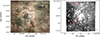 |
Fig. 1 Left: total 2′× 2′ field observed with MUSE (black square) overlaid on a colour-composite image of the central 7.3′ × 6′ (≈110 × 90 pc) of the Tarantula Nebula obtained with the Wide Field Imager (WFI). The young star cluster R136 is indicated at the centre, with R140, an aggregate of W–R stars, to the north and Hodge 301, the older cluster, to the north-west. Right: continuum-integrated (4600–9300 Å) MUSE mosaic. |
3 Stellar content of NGC 2070
We extracted spectra from the reduced MUSE cubes using detections of 2255 sources from SExtractor (Bertin & Arnouts 1996) on the continuum-integrated mosaic shown in the right-hand panel of Fig. 1 (constructed using the 600 s frames). The extracted MUSE sources are listed (in ascending right ascension) in Table 3, where Cols. 2 and 3 give previous identifications from Selman et al. (1999) and Evans et al. (2011), respectively. Given the resolved ISM structures and stellar crowding in the region, we estimate the sky contribution locally to each source, adopting annuli with inner radii of 7 pixels and a radial width of 1 pixel. Even with this approach, the complex nebulosity and nearby stars still thwart ideal sky subtraction in many cases.
We were relatively conservative in the extraction of sources, in the sense that there were several hundred additional sources detected by SExtractor where the MUSE magnitudes and spectra wereprobably contaminated by nearby stars. We note that R136 was not explicitly excluded from the SExtractor analysis, but that very few sources were detected because of the significant crowding.
3.1 Photometry
Johnson V - and I-band photometry is obtained for each MUSE source using the relative fluxes from the pipeline. To estimate the V -band zero-point, we compared the instrumental MUSE magnitudes with published photometry for matched sources from Selman et al. (1999), as shown in the left-hand panel of Fig. 2. A zero-point correction of −0.6 mag is necessary to shift the MUSE photometry to the Selman et al. (1999) data (Weilbacher et al. 2015). The scatter at faint magnitudes probably arises from issues with background subtraction, that is, contamination by nearby stars (particularly around R136). Selman et al. (1999) observed NGC 2070 with UBV filters, and in absence of comparable I-band data, we therefore estimated (V − I)MUSE on the basis of the relative flux calibration from the spectrophotometric standards observed with MUSE.
The estimated MUSE magnitudes and colours are included in Table 3; 1147 sources have VMUSE < 21.5. The right-hand panel of Fig. 2 compares the distribution of V -band magnitudes of the MUSE sources to ground-based photometry from Parker (1992) and Selman et al. (1999). The MUSE observations go deeper, but are more limited by crowding at the brighter end. This is not surprising given the typical PSF of the MUSE data; see the ≈0.7″ obtained by Selman et al. (1999) in the V band2.
The locations of our extracted MUSE sources in a colour-magnitude diagram are shown in Fig. 3 compared to isochrones spanning 1 Myr to 1 Gyr from PARSEC stellar evolution models for the metallicity of the LMC, which include both pre-main- sequence and main-sequence phases (Bressan et al. 2012)3. As expected, Fig. 3 illustrates the significant population of luminous blue stars that is compatible with ages of a few Myr. Figure 3 is also consistent with a significant pre-main-sequence population (with 20 ≤V ≤ 22 and (V − I) ≈ 1) with ages of a few Myr (see e.g. Cignoni et al. 2015; Sabbi et al. 2016; Khorrami et al. 2017). Figure 3 does not allow distinguishing multiple young bursts (Walborn & Blades 1997; Massey & Hunter 1998), although older populations are also present in NGC 2070 (e.g. a few cool supergiants with ages of ≈30 Myr). We note that Sabbi et al. (2016) reported evidence for an older underlying stellar population (see also Harris & Zaritsky 2009). This is part of the local field population of the LMC and could influence the analysis of the pre-main-sequence stars.
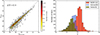 |
Fig. 2 Left: calibration of MUSE V -band magnitudes compared with photometry from Selman et al. (1999); the solid black line indicates the 1:1 ratio. Right: magnitude distribution of stars extracted from the MUSE data (and shifted by −0.6 mag to match Selman et al. 1999); the corresponding distributions for the MUSE area from Parker (1992) and Selman et al. (1999) are shown for comparison. |
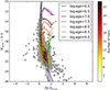 |
Fig. 3 Colour–magnitude diagram for the extracted MUSE sources compared with isochrones from PARSEC evolutionary models (Bressan et al. 2012); the ages quoted are in years. |
3.2 Spectroscopy
The MUSE observations provide intermediate-resolution spectroscopy at S∕N ≥ 50 for 588 stars (from the 4 × 600 s exposures). The observed wavelength range includes the primary classification diagnostics of Of/WN and W–R stars (except for N IV 4058), but not the features used for the majority of early-type stars (e.g. Walborn & Fitzpatrick 1990; Castro et al. 2008, 2012). Nonetheless, the MUSE data are expected to permit robust classifications through alternative diagnostics. For O-type stars the spectra include several He I (λλ4713, 4921, 5876, 6678) and He II (λλ5412, 6683) transitions, as well as N III λλ4634–41, N IV λλ7103–29, N V λλ4603–20, C III λλ4647–51, λ5696, C IV λλ5801–12, and O III λ5592. The Hβ and Hα lines are also included, but are often severely affected by nebulosity and issues related to sky substraction. For B-type stars there are additional useful He I lines, as well as N II λλ4601–43, λλ5667–5701, O II λλ4639–76, and Si III λ5740.
Illustrative MUSE spectra over the range 4600–6000 Å are shown in Fig. 4 for eight O- and early B-type stars previously classified by Walborn et al. (2014) and Evans et al. (2015); the relevant diagnostic lines are indicated. We note that the sky subtraction can give residuals in the [O III] λλ4959, 5007 lines, and can similarly influence the appearance of Hβ. Classification and quantitative analysis of this large dataset of early-type stars requires implementation of automated techniques, and results on this aspect of the MUSE data will be reported in a separate article.
It is well established that NGC 2070 contains a number of early-type stars with strong emission lines (Melnick 1985). Figure 5 shows a net He IIλ4686 image from the MUSE data, obtained by subtracting the local continuum (λλ4740–60) from the emission between λλ4680–4700. Each of R136a (containing several WN and Of/WN stars), R140a (WN + WC), R140b (WN), and R134 (WN6) are prominent, together with several WN stars (Mk 34, R136c, Mk 49, Mk 53), Of/WN stars (Mk 39, Mk 51, R136b), Of stars (Mk 42, Mk 37), and a WC star (Mk33Sb). The observed emission-line fluxes of He II λ4686, N III λ4640+C IIIλ4650, C IV λ5808, and Hα for these sources are presented in Table 2, illustrating that several W–R stars contribute to the cumulative λ4686 emission, with two WC stars (R140a1, Mk33Sb) dominating the λ4640–50 emission. From across the entire NGC 2070 region, R140a1 provides the dominant contribution to both the blue W–R bump and the C IV λλ5801–12 W–R feature.
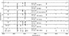 |
Fig. 4 Illustrative O- and early B-type spectra from the MUSE observations, with classifications from Walborn et al. (2014) and Evans et al. (2015). The relevant lines for spectral classification are labelled, as is the location of the nebular [O III] lines (which show residuals from over- and under-subtraction of the local nebulosity). |
Dominant stellar emission-line sources within the MUSE observations of NGC 2070, with identifications from Breysacher et al. (1999, BAT99), Feast et al. (1960, R), Melnick (1985, Mk), Evans et al. (2011, VFTS), and the MUSE data.
4 Ionised gas in NGC 2070
The MUSE data also provide a wealth of spatially resolved information on the nebular content of NGC 2070. The integrated spectrum from the MUSE cubes is shown in Fig. 6, displaying very strong Hα, Hβ, and [O III] λλ4959, 5007 emission, and with prominent emission from He Iλ5876, 6678, [N II] λλ6548–83, and [S II] λλ6717, 6731. Broad emission is present around He IIλ4686 as a result of the strong contribution from the population of W–R stars in NGC 2070 (see Fig. 5).
We nowdiscuss the spatial distribution of the ionised gas in NGC 2070, based on the low-ionisation diagnostic lines (Hα and [N II] λ6583.45, hereafter [N II]); the gas kinematics are discussed in Sect. 5. The Hα emission was saturated in large areas of the 600 s exposures, therefore maps were created using single-component Gaussian fits to the 4 × 60 s exposures. This gave S∕N > 50∕pix. across the entire MUSE mosaic for both lines. From similar Gaussian fits to the relevant emission lines we also constructed maps of the interstellar extinction, electron density, and temperature using standard nebular techniques.
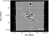 |
Fig. 5 Net He II λ4686 emission in the MUSE mosaic of NGC 2070, highlighting the W–R content of R136 and R140, and other emission-line sources. The source north-east of R136, which is brighter in the continuum (cf. λ4686), is the M-type supergiant Mk 9. |
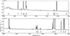 |
Fig. 6 Integrated spectrum (4600–6800 Å) from the MUSE mosaic; prominent emission lines are labelled. |
4.1 Intensity of Hα and [N II] emission
The Hα and [N II] emission in the MUSE mosaic reveal the ionised gas and structure of the ISM in NGC 2070, as shown in the upper panels of Fig. 7 (see also Walborn et al. 2002b). These include a ≈ 1′ × 30″ (≃ 15 × 7 pc) cavity to the east of R136 and a large shell to the west with an angular size of 1′ (≃15 pc). In the north-eastern part of the images is the so-called eastern filament, which includes Knot 1 (see Walborn & Blades 1997; Walborn et al. 1999).
The [N II] flux is significantly lower than that from Hα, but the S/N is sufficient for robust detection across the entire MUSE mosaic (except for some regions, e.g. around R140, where strong Hα emission masks the [N II]). The [N II] emission mimics the structures seen in Hα, but appearsto be in more discrete clumps. These are generally associated with individual sources, such as W–R stars within the cluster core (Fig. 5). The [N II] map reveals many individual clumps in the various ISM filaments, which probably trace current stellar nurseries (as suggested by Walborn & Blades 1997). We note two isolated regions in the south-eastern part of the [N II] map with remarkable bullet-shaped morphologies4, perhaps indicative of runaway phenomena.
4.2 FWHM of Hα and [N II] emission
The lower panels of Fig. 7 present the full-width at half-maxima (FWHM) of single-component Gaussian fits to both the Hα and [N II] lines. The MUSE data appear to reveal a series of seemingly broad components in the eastern cavity, although we caution that the velocity resolution of MUSE at Hα is ≈100 km s−1, which means that multiple velocity components may be unresolved. Past observations of NGC 2070 at higher spectral resolution have indeed revealed rich sub-structures (e.g. Melnick et al. 1999; Torres-Flores et al. 2013). The multi-component structures seen previously are outside the MUSE mosaic, but are close to the eastern edge of our data where the FWHM shows the highest values. Moreover, the multi-component composition of the ISM in the cavity was recently reported by Mendes de Oliveira et al. (2017) from Fabry-Perot observations.
The large FWHM in Fig. 7 also appears to trace the border between R136 and the cavity, potentially a consequenceof the radiation pressure from massive stars in R136 (Townsley et al. 2006a; Pellegrini et al. 2011). In contrast, the distribution of FWHM estimates in the west (sampling the large shell) are more comparable with the velocity resolution of MUSE.
Figure 7 indicates several compact regions (in the eastern cavity and elsewhere) with high FWHM estimates (≥250 km s−1). These are probably associated with stars with dense, complex circumstellar material, and were also reported by Mendes de Oliveira et al. (2017). For example, Mk 95 (MUSE 2658), the red supergiant in the northern part of the cavity, shows a large FWHM in the Hα map, possibly the externally photoionised wind (Mackey et al. 2015a). A number of the W–R stars in the mosaic also appear to have high FWHM values, which arise from the contribution of broad Hα emission from their stellar winds to the nebular component.
For completeness, we note that the Tarantula Nebula has been imaged with near-IR narrow-band filters (H2 2.12 μm and Br γ 2.17 μm) with the NEWFIRM camera on the 4m Blanco telescope on Cerro Tololo (Yeh et al. 2015). Inspection of these images (kindly provided by the authors) revealed morphological features or trends similar to those discussed above.
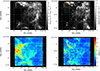 |
Fig. 7 Relative Hα (left) and [N II] λ6583.45 (right) fluxes (upper panels) and full-width at half-maxima (lower panels) extracted from single-component Gaussian fits to both lines in the MUSE datacubes. The red circle indicates the core of R136. |
4.3 Extinction map
The strong nebular emission in NGC 2070 permits estimates of interstellar extinction from the Hα/Hβ ratio, assuming Case B recombination theory for ne = 100 cm−3 and Te = 10 000 K, that is, an intrinsic ratio of I(Hα)/I(Hβ) = 2.86 (Hummer & Storey 1987). We adopted a standard extinction law (Cardelli et al. 1989) with RV = 3.1 in our calculations to ensure a direct comparison with Pellegrini et al. (2010). Figure 8 shows c(Hβ) across the MUSE mosaic, with a broad range of extinctions (0.15 ≤ c(Hβ) ≤ 1.2), and where foreground extinction due to the Milky Way is c(Hβ) ≈ 0.1. The average c(Hβ) of 0.55 mag equates to E(B − V) ≈ 0.38 (≃0.7 c(Hβ)), in excellent agreement with Pellegrini et al. (2010).
The extinction map in Fig. 8 shows a complex distribution, but resembling the large ISM clouds highlighted by the Hα intensity map (Fig. 7), for example, lower extinction in the eastern cavity. Several regions of high extinction are seen to the south-west, but with no obvious counterparts in the Hα map. The low extinction toward several of the W–R stars in the region (relative to their local environment, see sources labelled in Fig. 8) appears remarkable. This suggests that their stellar winds and/or ionising radiation could have influenced their immediate ISM. While the extinction determinations near these W–R stars may be influenced by extended stellar emission at Hα and Hβ, note that we do not see a similar behaviour toward other W–R stars in the MUSE data.
Recent studies have demonstrated that the extinction law in 30 Doradus is anomalous (Doran et al. 2013; Maíz Apellániz et al. 2014; De Marchi & Panagia 2014), with RV ≈ 4.4, indicating higher total extinction and with implications for nebular diagnostics. Recalculating for RV = 4.4 and an extinction law of the form from Maíz Apellániz et al. (2014), we find an average c(Hβ) of ≈0.60 mag. Given our use of relatively red diagnostic lines (and with small separation in terms of wavelength), this has a minimum effect on our calculations of temperature and density in the following section.
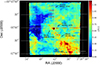 |
Fig. 8 Reddening coefficient c(Hβ) across NGC 2070. Five W–R stars with low c(Hβ) values are labelled (see Sect. 4.3 and Table 2). |
4.4 Density and temperature distribution
The nebular lines observed in our MUSE datacube (see Fig. 6) can be used to construct maps of the electron density and temperature (e.g. McLeod et al. 2015). The electron density was estimated from the [S II] λ6717/6731 ratio following the parameterisation of McCall (1984), with the average ratio implying a mean density of ≈230 cm−3. The left-hand panel of Fig. 9 presents the range of densities in the MUSE data, spanning 50–1000 cm−3, which agrees reasonably well with Pellegrini et al. (2010). The densest regions correspond to sites of on-going stellar formation and high densities of CO (Johansson et al. 1998). There are several dense regions to the south, mainly in the tip of structures that resemble the pillars in M 16.
Figure 9 also indicates the six sources in the MUSE mosaic classified as “definite”, “probable”, or “possible” young stellar objects (YSOs) by Gruendl & Chu (2009). Four of these coincide with relatively dense regions: Knot 1 (Walborn & Blades 1997), Knot 3 (Walborn et al. 1999), and a bullet-shaped clump around the YSO candidate close to R134 (cf. Fig. 8) that might be shaped by the powerful stellar wind from this WN6 star.
The absence of [O III] λ4363 from the MUSE dataset led us to use the [N II] λλ6548, 6584/5755 and [S III] λλ9069/6312 ratios (after correction for extinction) to estimate the electron temperature, using the calibration of Osterbrock & Ferland (2006). The right-hand panel of Fig. 9 presents the electron temperature map of NGC 2070 based on the [N II] line ratios, which rangefrom 9000 to 12500 K, in agreement with the range estimated by Pellegrini et al. (2010) using the [O III] λλ4959, 5007/4363 ratio. The average intensity ratio of [N II] λλ6548, 6584/5755 gave a mean temperature of ≈11 000 K. The weakness or absence of [N II] λ5755 prevented estimates in some areas (black patches in the map); the noisy temperature distribution arises from the general weakness of [N II] λ5755. High electron temperatures are associated with the densest regions to the north, west, and south. The [S III] λ9069/6312 intensity ratio provided an average temperature of ≈9800 K.
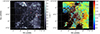 |
Fig. 9 Left: electron density map derived from the [S II] λ6717/6731 ratio. Candidate young stellar objects from Gruendl & Chu (2009) are indicated by the red open circles, and Knots 1 and 3 from Walborn et al. (2002b) are also identified. Right: electron temperature map derived from the [N II] lines. |
5 Kinematics
5.1 Nebular velocity distribution
The mean radial velocity estimated from our single-component Gaussian fits to the Hα and [N II] nebular lines was 265 km s−1 (cf. 266 ± 8 km s−1 from Hénault-Brunet et al. 2012a). We adopted this as our systemic value, and differential velocities across the MUSE mosaic are shown for both lines in Fig. 10.
The estimated (absolute) velocities for the emission lines in each of the extracted MUSE sources are listed in Cols. 8 and 9 of Table 3. These are effectively the average of the peak emission in the pixels across each ≈1″ radius aperture, and we estimate a pixel-to-pixel accuracy of 1.5–2 km s−1 (see also Weilbacher et al. 2015). The nebular velocities for some sources have larger dispersions, which probably are spatially resolved velocity structures within the extracted apertures and not poor precision (see the complexity of the maps in Fig. 10).
Some areas in the MUSE mosaic have differential velocities greater than the range shown in Fig. 10 (i.e. |δv| > 40 km s−1), but we adopted the intensity scale to highlight the general distribution. As noted by Pellegrini et al. (2010), there are well-defined regions of both blue- and red-shifted material in Fig. 10, but the details and spatial sampling of MUSE are striking. The ionised gas to the west of R136 is approaching us, while the gas to the north-east of R136 is mostly receding, as noted by Chu & Kennicutt (1994). We also find a good match with the Mendes de Oliveira et al. (2017) velocity measurements despite their higher spectral resolution.
The highest blue-shifted velocities roughly shape the shell in the Hα velocity map with peaks of ≈ −35 km s−1 (and ≈ −45 km s−1 for [N II]). Knot 3 from Walborn et al. (1999), labelled in Fig. 9, is located in one of the most strongly blue-shifted regions. Radiation pressure, stellar winds, and/or former supernovae could have compressed the materialproducing this large shell structure (e.g. Rosen et al. 2014, and references therein). Assuming a symmetric phenomenon, one might anticipate blue-shifted material elsewhere around R136 (although projection effects should be borne in mind), but this is not the case. The dense gas in the north-eastern region has intense Hα and [N II] emission (Fig. 7), but with a similar radial velocity as the core of R136. Gas in the eastern cavity is predominantly red-shifted by 25–40 km s−1.
Beyond Knot 3, there are several other features of note in the western shell. There are two sources at approximately α = 5h38m39s and δ =−69°06′10″ in the [N II] map (see the western edge of the right-hand panel of Fig. 11). Bi-modal red- and blue-shifted material is seen, which is suggestive of either rotation or ejecta, with velocities of ≈13 to −40 km s−1 for the northern feature. Given the ongoing star formation in NGC 2070, such phenomena are not unexpected (e.g. McLeod et al. 2015), although we note that while they are nearby, they are not part of the brightest stellar nurseries in the western shell that we mentioned in Sect. 4.1.
Red-shifted velocities are predominantly located on the south-eastern side of R136 and in the optical cavity in the ISM on the eastern side of the MUSE mosaic. In an optically thin environment (see Sec. 4.3), we could be observing background layers of 30 Dor where the material is receding, but the cavity does not show a homogeneous recession velocity. Only a portion is receding (although some parts recede at more than 50 km s−1), with some of it approaching us.
High velocities are found in the Hα map around several sources in the cavity, which is clearly seen in the [N II] velocity map. As highlighted in Sect. 4.2, this coincides with a large FWHM in the emission as well, and unresolved components probably play a role (cf. e.g. Torres-Flores et al. 2013). Mendes de Oliveira et al. (2017) also reported high-velocity clouds in the cavity. Broad and/or multiple components are probably influencing our estimated velocities for this and other objects, and high-resolution spectroscopy is required to separate the different kinematic structures.
The overall spatial distribution of radial velocities is intriguing and poses the question of whether localised independent phenomena or a single mechanism dominate the behaviour. The largest red- and blue-shifted velocities are qualitatively aligned with the core of R136, along an axis almost perpendicular to the western shell; a rotation of the ISM around this axis would induce a bi-modal radial-velocity distribution. There is marginal evidence to date for rotation in young clusters (e.g. Fischer et al. 1993; Davies et al. 2011), but we note the finding of Hénault-Brunet et al. (2012b) of potential rotation of the O-type stars of R136 with an amplitude of ≈3 km s−1. This is much lower than the apparent difference in ISM velocities across R136, although not a like-for-like comparison, as the ISM analysis extends farther out into NGC 2070. Nonetheless, the proposed rotational axis from Hénault-Brunet et al. (2012b) appears somewhat offset from that suggested by our ISM measurements (see Fig. 10).
External factors acting on NGC 2070, combined with the outward pressure from the young stellar population of R136, might offer an alternative mechanism. Schneider et al. (2012) showed that most star clusters form at the junction of filaments in molecular clouds, and André et al. (2014) reviewed the evidence from theory and observations that converging filaments provide sufficient mass flux onto the filament junction to allow a star cluster to form. In this paradigm of massive cluster formation, we expect 30 Dor to be fed by a number of accreting filaments of molecular gas. In the time since the cluster has formed, feedback processes (winds and supernovae) have created a hot bubble of high-pressure, X-ray emitting gas around R136, and this prevents further accretion of dense gas onto the cluster (e.g. Pellegrini et al. 2011). R136 is at the centre of a young superbubble that is being formed by feedback processes from its stars (Chu & Kennicutt 1994).
The result is that the star cluster could be embedded in a stream of dense gas that is forced to flow around it, a well-known physical phenomenon explored at different astropysical scales (e.g. Shaviv & Salpeter 1982; Mackey et al. 2015b). The ISM may collide with the hot bubble surrounding R136 and encircle the cluster, producing a ram-pressure effect and moving the ISM toward the observer, consistent with production of the western shell.
Furthermore, the feedback from massive stars in R136 has swept up a massive (65 000 M⊙, Chu & Kennicutt 1994) dense shell that is expanding outwards at up to 40 km s−1. This expanding shell would decelerate and entrain any ISM that would be flowing towards R136. The observed eastern cavity may be a lower-density part of the ISM, where there were no accreting filaments. Under this hypothesis, the mean flow of gas would then be from west to east, and the cavity is a low-density wake downstream from R136. The dent in the CO maps around R136 reported by Johansson et al. (1998, see their Fig. 1, for instance,) may be a consequence of the strong UV radiation as they suggested, but would also support the idea of differential movement between R136 and the ISM.
Moreover, the eastern cavity has much lower extinction than the western side, suggesting that the expanding shell around R136 is incomplete in the hemisphere closer to us. The Hα emitting gaswould then be mainly emitted from the far side of the shell, explaining why it is strongly red-shifted. This hypotheticalscenario will be tested in future works.
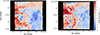 |
Fig. 10 Radial-velocity maps from Gaussian fits to the Hα and [N II] λ6583 emission (left and right panels, respectively). The core of R136 is indicated with the red open circle, and the black dashed line is the proposed rotational axis from Hénault-Brunet et al. (2012b), see Sect. 5.1. |
5.2 Gas kinematics around R136
In addition to R140, the main X-ray sources in the MUSE mosaic are in R136 (Townsley et al. 2006a,b). The brightest X-ray sources are Mk 34 (WN5h), R136c (WN5h), and the R136a cluster (Schnurr et al. 2009), presumably involving colliding-wind binaries (Crowther et al. 2010). Periodic X-ray variability in Mk 34 consistent with a colliding-wind system has recently been discovered from observations with Chandra as part of the T-ReX project (Pollock et al. 2018). Figure 11 shows the central ≈40″ × 40″ (≃10 × 10 pc) of the Hα and [N II] velocity maps. Red-shifted material almost encircles the X-ray detections, which is particularly prominent on the eastern side of the cluster. The projected red-shifted ISM component, observed in Fig. 10, extends from the east side of the field to the core of R136. Blue-shifted material around the core of R136 may trace escape channels for the radiation pressure. Although the FWHM map does not appear to show blended clouds (see Fig. 7) and/or largely broad profiles around the core (as it does in the cavity), a composite spectrum is expected in the cluster core (Melnick et al. 1999), but will be unresolved in the MUSE data.
We would expect the rich population of massive stars in R136 to be driving material away as a result of their combined intense stellar winds. The ISM apparently moves toward the core of R136 (cf. the systemic velocity of the cluster). However, the projected red-shifted material on R136a could be either a foreground/background ISM projection, or it might mean that the radial velocity of R136a is higher than the average systemic velocity of NGC 2070.
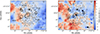 |
Fig. 11 Radial-velocity estimates for the peak Hα and [N II]emission (left- and right-hand panels, respectively) in the vicinity of R136 at the centre of the MUSE mosaic. Contours mark the most prominent X-ray sources from Chandra 1.1–2.3 KeV imaging (Townsley et al. 2006a,b), with the strongest sources labelled in the left-hand panel. Velocities are plotted on the same scale as in Fig. 10. The average PSF of the MUSE data (≈1″) is indicated in the right-hand panel by the green dot in the south-eastern corner. |
5.3 Stellar velocity distribution
To investigate stellar radial velocities, we used the He II λ5411.5 line in the O-type spectra (and some of the earliest B-type spectra, see Fig. 4); using the He II line has the advantage that it is free of potential nebular contamination; compare the He I lines in the more numerous B-type stars. Estimated radial velocities are given in Table 3 for 270 stars, with an average of 271 ± 41 km s−1 (in agreement with the systemic value of the ISM and stellar results from Hénault-Brunet et al. 2012a). The uncertainties quoted on the velocities in Table 3 are the standard deviations of each pixel within the extracted aperture.
From an analysis of 38 (apparently non-variable) O-type stars, Hénault-Brunet et al. (2012a) concluded that the core of R136 was in virial equilibrium with a line-of-sight velocity dispersion of no more than 6 km s−1. In this context, the large dispersion of41 km s−1 from our estimates probably reflects the limits of the velocity resolution from MUSE (and the S/N of our spectra), combined with undetected binaries (see Bosch et al. 2009; Hénault-Brunet et al. 2012a). The distribution of stellar radial velocities is shown in Fig. 12, compared with estimates from the nebular Hα and [N II] atthe same positions. The large dispersion potentially arising from undetected binaries (and the lower S/N of the He II absorption; cf. the strong emission lines) precludes an obvious link between the stellar and gas components.
The (spatially limited) view of the ISM dynamics in Fig. 12 agrees reasonably well with the rotational axis proposed byHénault-Brunet et al. (2012b). However, as noted earlier from consideration of the full spatial information (Fig. 10), the true picture with regard to potential rotation of R136 is likely more complicated. Somewhat surprisingly, we note that the direction of the velocity gradient of the gas in Fig. 12 is inverted; compare the stellar results from Hénault-Brunet et al. (2012b; gas red-shifted more in the south-east, stars more so in the north-west). In short, although the ISM and stellar population have comparable average velocities in space, the potentially differential movement of these components could add support to the hypothesis that external mechanisms shape the dynamics of the ISM.
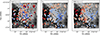 |
Fig. 12 Radial-velocity estimates from He IIλ5411.5 (left-hand panel) for 270 early-type stars compared with estimates from the Hα and N II λ6583.45 nebular lines superimposed on the spectra (central and right-hand panels, respectively). The colour of each hexagon indicates the median velocity of the sources in that area and follows the same scale as in Fig. 10. The black dashed line in each panel is the rotational axis proposed by Hénault-Brunet et al. (2012b). |
6 Summary
We introduced VLT-MUSE observations of the central 2′ × 2′ of NGC 2070 within the Tarantula Nebula in the LMC. The data permit a homogeneous spectroscopic census of the massive stars and ionised gas in the vicinity of the central star cluster R136.
We provide a catalogue of 2255 point sources detected in the MUSE mosaic, and include V - and I-band magnitudes estimated from the datacubes. The colour–magnitude diagram reveals a young bright population and a fainter group of stars, with the latter matching the predicted location of pre-main-sequence stars (e.g. Bressan et al. 2012). Both populations are compatible with a recent burst of star formation spanning a few Myr, as proposed in recent studies (e.g. Cignoni et al. 2015; Crowther et al. 2016). We also revisited the known W–R population in the region and their fluxes in some of the most prominent emission lines.
We constructed the extinction map for NGC 2070 from the ratio of Hα/Hβ, a map of electron densities based on [S II] lines, and the electronic temperature distribution maps from relative ratios of the [N II] and [S III] lines. The average electron density (230 cm−3) and temperature (11 000 K and 9800 K, based on [N II] and [S III], respectively) agree with those from Pellegrini et al. (2010), but the spatial resolution provided by MUSE gives new insights into the structure of the ISM and ongoing star formation in NGC 2070. We resolved several high-density clumps that are probably linked to the formation of new stars, some of which have previously been classified as candidate young stellar objects (Walborn et al. 2002b; Gruendl & Chu 2009). The electron temperature map shows higher temperatures close to these dense areas.
The structural features in the ISM of the region were investigated using Gaussian fits to the Hα and [N II] λ6583 nebular emission lines. The Hα emission traces several known structures in NGC 2070: a prominent shell in the west, several filaments in the north ofthe field, and a cavity to the east of R136. The extinction map resembles these structures, but we find several areas of high extinction in the south-west of the field without counterparts in the Hα map. The [NII] emission map shows a more clumpy distribution (similar to the high-density areas traced by the electron-density map) and is probably related to active sites of star formation.
We estimate a systemic velocity for the ISM of 265 km s−1 (in agreement with previous studies), butthe velocity maps for Hα and [N II] show complex kinematics in the region. We find a bi-modal, blue- and red-shifted distribution in the gas velocities centred on R136; the western shell is mainly blue-shifted, with material in the eastern cavity receding (e.g. Chu & Kennicutt 1994). This bi-modality does not match the velocities and rotational axis for stars in R136 from Hénault-Brunet et al. (2012b), but differential velocities between the stellar cluster and the ISM might arise from the effects of ram pressure.
Within our velocity maps we find several interesting point sources that might be related to stellar runaways, jets, the formation ofnew stars, or interaction of the gas with the W–R stars, and warrant further study. Closer inspection of the central region reveals red-shifted material encircling the diffuse X-ray emission, and reaching as far as R136a in the core. This could point to a more complex kinematics that are unresolved in these data. Several blue-shifted clumps around R136 suggest escape channels for the hot gas and radiation.
We estimate radial velocities of 270 O-type stars, finding an average of 271 ± 41 km s−1. The stellar velocities broadly match those of the ISM, but the spectral resolution of the data and likely presence of undetected binary components limits further analysis of the stellar dynamics.
Future papers on these data will focus on the stellar content of NGC 2070 and its integrated stellar and nebularproperties (Crowther et al. 2017). Given that the MUSE mosaic would only subtend 0.6″ at a distance of 10 Mpc (comparable to long-slit spectroscopy of extragalactic H II regions with large ground-based telescopes), the integrated properties will be of interest as they provide a template with which to investigate extragalactic systems.
Acknowledgements
The authors thank the referee for useful comments and helpful suggestions that improved this manuscript. We would like to thank S. Yeh for kindly providing near-IR images taken with the NEWFIRM camera on the Blanco telescope on Cerro Tololo (Chile). We thank Anna McLeod for her thoughts on the manuscript and ideas for future directions. JM acknowledges funding from a Royal Society–Science Foundation Ireland University Research Fellowship. This research made use of Astropy, a community-developed core Python package for Astronomy (Astropy Collaboration et al. 2013), and APLpy, an open-source plotting package for Python (Robitaille & Bressert 2012).
References
- André, P., Di Francesco, J., Ward-Thompson, D., et al. 2014, Protostars and Planets VI (Tucson: University of Arizona Press), 27 [Google Scholar]
- Astropy Collaboration, Robitaille, T. P., Tollerud, E. J., et al. 2013, A&A, 558, A33 [NASA ADS] [CrossRef] [EDP Sciences] [Google Scholar]
- Bacon, R., Vernet, J., Borisova, E., et al. 2014, The Messenger, 157, 13 [NASA ADS] [Google Scholar]
- Bertin, E., & Arnouts, S. 1996, A&AS, 117, 393 [NASA ADS] [CrossRef] [EDP Sciences] [Google Scholar]
- Bosch, G., Terlevich, E., & Terlevich, R. 2009, AJ, 137, 3437 [NASA ADS] [CrossRef] [Google Scholar]
- Bressan, A., Marigo, P., Girardi, L., et al. 2012, MNRAS, 427, 127 [NASA ADS] [CrossRef] [Google Scholar]
- Breysacher, J., Azzopardi, M., & Testor, G. 1999, A&AS, 137, 117 [NASA ADS] [CrossRef] [EDP Sciences] [Google Scholar]
- Cardelli, J. A., Clayton, G. C., & Mathis, J. S. 1989, ApJ, 345, 245 [NASA ADS] [CrossRef] [Google Scholar]
- Castro, N., Herrero, A., Garcia, M., et al. 2008, A&A, 485, 41 [NASA ADS] [CrossRef] [EDP Sciences] [Google Scholar]
- Castro, N., Urbaneja, M. A., Herrero, A., et al. 2012, A&A, 542, A79 [NASA ADS] [CrossRef] [EDP Sciences] [Google Scholar]
- Chu, Y.-H., & Kennicutt, Jr. R. C. 1994, ApJ, 425, 720 [NASA ADS] [CrossRef] [Google Scholar]
- Cignoni, M., Sabbi, E., van der Marel, R. P., et al. 2015, ApJ, 811, 76 [NASA ADS] [CrossRef] [Google Scholar]
- Cignoni, M., Sabbi, E., van der Marel, R. P., et al. 2016, ApJ, 833, 154 [NASA ADS] [CrossRef] [Google Scholar]
- Crowther, P. A., & Walborn, N. R. 2011, MNRAS, 416, 1311 [NASA ADS] [CrossRef] [MathSciNet] [Google Scholar]
- Crowther, P. A., Schnurr, O., Hirschi, R., et al. 2010, MNRAS, 408, 731 [NASA ADS] [CrossRef] [Google Scholar]
- Crowther, P. A., Caballero-Nieves, S. M., Bostroem, K. A., et al. 2016, MNRAS, 458, 624 [NASA ADS] [CrossRef] [Google Scholar]
- Crowther, P. A., Castro, N., Evans, C. J., et al. 2017, The Messenger, 170, 40 [Google Scholar]
- Cutri, R. M., Skrutskie, M. F., van Dyk, S., et al. 2003, VizieR Online Data Catalog: II/246 [Google Scholar]
- Davies, B., Bastian, N., Gieles, M., et al. 2011, MNRAS, 411, 1386 [NASA ADS] [CrossRef] [Google Scholar]
- de Koter, A., Heap, S. R., & Hubeny, I. 1998, ApJ, 509, 879 [NASA ADS] [CrossRef] [Google Scholar]
- De Marchi, G., & Panagia, N. 2014, MNRAS, 445, 93 [NASA ADS] [CrossRef] [Google Scholar]
- Doran, E. I., Crowther, P. A., de Koter, A., et al. 2013, A&A, 558, A134 [NASA ADS] [CrossRef] [EDP Sciences] [Google Scholar]
- Evans, C. J., Taylor, W. D., Hénault-Brunet, V., et al. 2011, A&A, 530, A108 [NASA ADS] [CrossRef] [EDP Sciences] [Google Scholar]
- Evans, C. J., Kennedy, M. B., Dufton, P. L., et al. 2015, A&A, 574, A13 [NASA ADS] [CrossRef] [EDP Sciences] [Google Scholar]
- Feast, M. W., Thackeray, A. D., & Wesselink, A. J. 1960, MNRAS, 121, 337 [NASA ADS] [CrossRef] [Google Scholar]
- Fischer, P., Welch, D. L., & Mateo, M. 1993, AJ, 105, 938 [NASA ADS] [CrossRef] [Google Scholar]
- Gruendl, R. A., & Chu, Y.-H. 2009, ApJS, 184, 172 [Google Scholar]
- Harris, J., & Zaritsky, D. 2009, AJ, 138, 1243 [NASA ADS] [CrossRef] [Google Scholar]
- Hénault-Brunet, V., Evans, C. J., Sana, H., et al. 2012a, A&A, 546, A73 [NASA ADS] [CrossRef] [EDP Sciences] [Google Scholar]
- Hénault-Brunet, V., Gieles, M., Evans, C. J., et al. 2012b, A&A, 545, L1 [NASA ADS] [CrossRef] [EDP Sciences] [Google Scholar]
- H.E.S.S. Collaboration (Abramowski, A., et al.) 2015, Science, 347, 406 [NASA ADS] [CrossRef] [Google Scholar]
- Hummer, D. G., & Storey, P. J. 1987, MNRAS, 224, 801 [NASA ADS] [CrossRef] [Google Scholar]
- Indebetouw, R., Brogan, C., Chen, C.-H. R., et al. 2013, ApJ, 774, 73 [NASA ADS] [CrossRef] [Google Scholar]
- Johansson, L. E. B., Greve, A., Booth, R. S., et al. 1998, A&A, 331, 857 [NASA ADS] [Google Scholar]
- Jones, T. A., Swinbank, A. M., Ellis, R. S., Richard, J., & Stark, D. P. 2010, MNRAS, 404, 1247 [NASA ADS] [Google Scholar]
- Kennicutt, Jr. R. C. 1984, ApJ, 287, 116 [NASA ADS] [CrossRef] [Google Scholar]
- Khorrami, Z., Vakili, F., Lanz, T., et al. 2017, A&A, 602, A56 [NASA ADS] [CrossRef] [EDP Sciences] [Google Scholar]
- Mackey, J., Castro, N., Fossati, L., & Langer, N. 2015a, A&A, 582, A24 [NASA ADS] [CrossRef] [EDP Sciences] [Google Scholar]
- Mackey, J., Gvaramadze, V. V., Mohamed, S., & Langer, N. 2015b, A&A, 573, A10 [NASA ADS] [CrossRef] [EDP Sciences] [Google Scholar]
- Maíz Apellániz, J., Evans, C. J., Barbá, R. H., et al. 2014, A&A, 564, A63 [NASA ADS] [CrossRef] [EDP Sciences] [Google Scholar]
- Massey, P., & Hunter, D. A. 1998, ApJ, 493, 180 [NASA ADS] [CrossRef] [Google Scholar]
- Matzner, C. D. 2002, ApJ, 566, 302 [NASA ADS] [CrossRef] [Google Scholar]
- McCall, M. L. 1984, MNRAS, 208, 253 [NASA ADS] [CrossRef] [Google Scholar]
- McLeod, A. F., Dale, J. E., Ginsburg, A., et al. 2015, MNRAS, 450, 1057 [NASA ADS] [CrossRef] [Google Scholar]
- Melnick, J. 1985, A&A, 153, 235 [NASA ADS] [Google Scholar]
- Melnick, J., Tenorio-Tagle, G., & Terlevich, R. 1999, MNRAS, 302, 677 [NASA ADS] [CrossRef] [Google Scholar]
- Mendes de Oliveira, C., Amram, P., Quint, B. C., et al. 2017, MNRAS, 469, 3424 [NASA ADS] [CrossRef] [Google Scholar]
- Mills, B. Y., Turtle, A. J., & Watkinson, A. 1978, MNRAS, 185, 263 [NASA ADS] [CrossRef] [Google Scholar]
- Osterbrock, D. E., & Ferland, G. J. 2006, Astrophysics of Gaseous Nebulae and Active Galactic Nuclei (Sausalito, CA: University Science Books) [Google Scholar]
- Parker, J. W. 1992, PASP, 104, 1107 [NASA ADS] [CrossRef] [Google Scholar]
- Pellegrini, E. W., Baldwin, J. A., & Ferland, G. J. 2010, ApJS, 191, 160 [NASA ADS] [CrossRef] [Google Scholar]
- Pellegrini, E. W., Baldwin, J. A., & Ferland, G. J. 2011, ApJ, 738, 34 [Google Scholar]
- Pietrzyński, G., Graczyk, D., Gieren, W., et al. 2013, Nature, 495, 76 [NASA ADS] [CrossRef] [PubMed] [Google Scholar]
- Pollock, A. M. T., Crowther, P. A., Tehrani, K., Broos, P. S., & Townsley, L. K. 2018, MNRAS, 474, 3228 [NASA ADS] [CrossRef] [Google Scholar]
- Robitaille, T., & Bressert, E. 2012, Astrophysics Source Code Library [record ascl:1208.017] [Google Scholar]
- Rosen, A. L., Lopez, L. A., Krumholz, M. R., & Ramirez-Ruiz, E. 2014, MNRAS, 442, 2701 [NASA ADS] [CrossRef] [Google Scholar]
- Sabbi, E., Anderson, J., Lennon, D. J., et al. 2013, AJ, 146, 53 [NASA ADS] [CrossRef] [Google Scholar]
- Sabbi, E., Lennon, D. J., Anderson, J., et al. 2016, ApJS, 222, 11 [NASA ADS] [CrossRef] [Google Scholar]
- Schneider, N., Csengeri, T., Hennemann, M., et al. 2012, A&A, 540, L11 [NASA ADS] [CrossRef] [EDP Sciences] [Google Scholar]
- Schnurr, O., Chené, A.-N., Casoli, J., Moffat, A. F. J., & St-Louis, N. 2009, MNRAS, 397, 2049 [NASA ADS] [CrossRef] [Google Scholar]
- Selman, F., Melnick, J., Bosch, G., & Terlevich, R. 1999, A&A, 341, 98 [NASA ADS] [Google Scholar]
- Shaviv, G., & Salpeter, E. E. 1982, A&A, 110, 300 [NASA ADS] [Google Scholar]
- Torres-Flores, S., Barbá, R., Maíz Apellániz, J., et al. 2013, A&A, 555, A60 [NASA ADS] [CrossRef] [EDP Sciences] [Google Scholar]
- Townsley, L. K., Broos, P. S., Feigelson, E. D., et al. 2006a, AJ, 131, 2140 [NASA ADS] [CrossRef] [Google Scholar]
- Townsley, L. K., Broos, P. S., Feigelson, E. D., Garmire, G. P., & Getman, K. V. 2006b, AJ, 131, 2164 [NASA ADS] [CrossRef] [Google Scholar]
- van Loon, J. T., Bailey, M., Tatton, B. L., et al. 2013, A&A, 550, A108 [NASA ADS] [CrossRef] [EDP Sciences] [Google Scholar]
- Walborn, N. R. 1991, in The Magellanic Clouds, eds. R. Haynes, & D. Milne, IAU Symp., 148, 145 [NASA ADS] [CrossRef] [Google Scholar]
- Walborn, N. R., & Blades, J. C. 1997, ApJS, 112, 457 [NASA ADS] [CrossRef] [Google Scholar]
- Walborn, N. R., & Fitzpatrick, E. L. 1990, PASP, 102, 379 [NASA ADS] [CrossRef] [Google Scholar]
- Walborn, N. R., Barbá, R. H., Brandner, W., et al. 1999, AJ, 117, 225 [NASA ADS] [CrossRef] [Google Scholar]
- Walborn, N. R., Howarth, I. D., Lennon, D. J., et al. 2002a, AJ, 123, 2754 [NASA ADS] [CrossRef] [Google Scholar]
- Walborn, N. R., Maíz-Apellániz, J., & Barbá, R. H. 2002b, AJ, 124, 1601 [NASA ADS] [CrossRef] [Google Scholar]
- Walborn, N. R., Barbá, R. H., & Sewiło, M. M. 2013, AJ, 145, 98 [NASA ADS] [CrossRef] [Google Scholar]
- Walborn, N. R., Sana, H., Simón-Díaz, S., et al. 2014, A&A, 564, A40 [NASA ADS] [CrossRef] [EDP Sciences] [Google Scholar]
- Weilbacher, P. M., Streicher, O., Urrutia, T., et al. 2012, Proc. SPIE, 8451, 84510B [NASA ADS] [CrossRef] [Google Scholar]
- Weilbacher, P. M., Monreal-Ibero, A., Kollatschny, W., et al. 2015, A&A, 582, A114 [NASA ADS] [CrossRef] [EDP Sciences] [Google Scholar]
- Yeh, S. C. C., Seaquist, E. R., Matzner, C. D., & Pellegrini, E. W. 2015, ApJ, 807, 117 [NASA ADS] [CrossRef] [Google Scholar]
Observations obtained under programme 076.C-0888, processed and released by the ESO VOS/ADP group.
We acknowledge that higher-resolution imaging of the region is available from the Hubble Tarantula Treasury Project (HTTP; Sabbi et al. 2013, 2016). Given the signficant difference in image quality, cross-matching between these data and the MUSE catalogue is non-trivial, often with multiple (and sometimes spurious) matches. Our primary interest here are the extracted MUSE spectra, therefore we did not employ the HTTP data further, but we caution that some of our sources will be multiples or composites if observed at finer angular resolution.
α ≈ 05h38m50s, δ ≈−69°06′39″.
α = 05h38m48. s480, δ =−69°05′32.′′58 (Melnick 1985; Cutri et al. 2003).
All Tables
Dominant stellar emission-line sources within the MUSE observations of NGC 2070, with identifications from Breysacher et al. (1999, BAT99), Feast et al. (1960, R), Melnick (1985, Mk), Evans et al. (2011, VFTS), and the MUSE data.
All Figures
|
Fig. 1 Left: total 2′× 2′ field observed with MUSE (black square) overlaid on a colour-composite image of the central 7.3′ × 6′ (≈110 × 90 pc) of the Tarantula Nebula obtained with the Wide Field Imager (WFI). The young star cluster R136 is indicated at the centre, with R140, an aggregate of W–R stars, to the north and Hodge 301, the older cluster, to the north-west. Right: continuum-integrated (4600–9300 Å) MUSE mosaic. |
| In the text | |
|
Fig. 2 Left: calibration of MUSE V -band magnitudes compared with photometry from Selman et al. (1999); the solid black line indicates the 1:1 ratio. Right: magnitude distribution of stars extracted from the MUSE data (and shifted by −0.6 mag to match Selman et al. 1999); the corresponding distributions for the MUSE area from Parker (1992) and Selman et al. (1999) are shown for comparison. |
| In the text | |
|
Fig. 3 Colour–magnitude diagram for the extracted MUSE sources compared with isochrones from PARSEC evolutionary models (Bressan et al. 2012); the ages quoted are in years. |
| In the text | |
|
Fig. 4 Illustrative O- and early B-type spectra from the MUSE observations, with classifications from Walborn et al. (2014) and Evans et al. (2015). The relevant lines for spectral classification are labelled, as is the location of the nebular [O III] lines (which show residuals from over- and under-subtraction of the local nebulosity). |
| In the text | |
|
Fig. 5 Net He II λ4686 emission in the MUSE mosaic of NGC 2070, highlighting the W–R content of R136 and R140, and other emission-line sources. The source north-east of R136, which is brighter in the continuum (cf. λ4686), is the M-type supergiant Mk 9. |
| In the text | |
|
Fig. 6 Integrated spectrum (4600–6800 Å) from the MUSE mosaic; prominent emission lines are labelled. |
| In the text | |
|
Fig. 7 Relative Hα (left) and [N II] λ6583.45 (right) fluxes (upper panels) and full-width at half-maxima (lower panels) extracted from single-component Gaussian fits to both lines in the MUSE datacubes. The red circle indicates the core of R136. |
| In the text | |
|
Fig. 8 Reddening coefficient c(Hβ) across NGC 2070. Five W–R stars with low c(Hβ) values are labelled (see Sect. 4.3 and Table 2). |
| In the text | |
|
Fig. 9 Left: electron density map derived from the [S II] λ6717/6731 ratio. Candidate young stellar objects from Gruendl & Chu (2009) are indicated by the red open circles, and Knots 1 and 3 from Walborn et al. (2002b) are also identified. Right: electron temperature map derived from the [N II] lines. |
| In the text | |
|
Fig. 10 Radial-velocity maps from Gaussian fits to the Hα and [N II] λ6583 emission (left and right panels, respectively). The core of R136 is indicated with the red open circle, and the black dashed line is the proposed rotational axis from Hénault-Brunet et al. (2012b), see Sect. 5.1. |
| In the text | |
|
Fig. 11 Radial-velocity estimates for the peak Hα and [N II]emission (left- and right-hand panels, respectively) in the vicinity of R136 at the centre of the MUSE mosaic. Contours mark the most prominent X-ray sources from Chandra 1.1–2.3 KeV imaging (Townsley et al. 2006a,b), with the strongest sources labelled in the left-hand panel. Velocities are plotted on the same scale as in Fig. 10. The average PSF of the MUSE data (≈1″) is indicated in the right-hand panel by the green dot in the south-eastern corner. |
| In the text | |
|
Fig. 12 Radial-velocity estimates from He IIλ5411.5 (left-hand panel) for 270 early-type stars compared with estimates from the Hα and N II λ6583.45 nebular lines superimposed on the spectra (central and right-hand panels, respectively). The colour of each hexagon indicates the median velocity of the sources in that area and follows the same scale as in Fig. 10. The black dashed line in each panel is the rotational axis proposed by Hénault-Brunet et al. (2012b). |
| In the text | |
Current usage metrics show cumulative count of Article Views (full-text article views including HTML views, PDF and ePub downloads, according to the available data) and Abstracts Views on Vision4Press platform.
Data correspond to usage on the plateform after 2015. The current usage metrics is available 48-96 hours after online publication and is updated daily on week days.
Initial download of the metrics may take a while.