| Issue |
A&A
Volume 614, June 2018
|
|
|---|---|---|
| Article Number | A141 | |
| Number of page(s) | 7 | |
| Section | Stellar structure and evolution | |
| DOI | https://doi.org/10.1051/0004-6361/201731308 | |
| Published online | 27 June 2018 | |
Complex long-term activity of the post-nova X Serpentis★
1
Astronomical Institute, The Czech Academy of Sciences,
25165
Ondřejov, Czech Republic
e-mail: This email address is being protected from spambots. You need JavaScript enabled to view it.
2
Czech Technical University in Prague, Faculty of Electrical Engineering,
16627
Prague, Czech Republic
Received:
3
August
2017
Accepted:
5
March
2018
Abstract
Aims. X Ser is a cataclysmic variable (CV) which erupted as a classical nova in 1903. In this work we use over 100 years of photometry to characterize the long-term light curve of X Ser, with the aim of interpreting the post-nova activity in X Ser in the context of behaviors in other old novae.
Methods. This analysis of its long-term optical activity uses the data from the Digital Access to a Sky Century @ Harvard (DASCH), AAVSO, and Catalina Real-time Transient Survey databases, supplemented by the data of other authors.
Results. We show that X Ser displays a strong complex activity with the characteristics of various CV types after the return to quiescence from its classical nova outburst. Both nova-like and dwarf nova (DN) features are present. The decaying branches of the individual post-nova outbursts display large mutual similarities and obey the Bailey law for outbursts of DNe. These outbursts of X Ser constitute a uniform group (inside-out outbursts), and their decaying branches can be explained by propagation of cooling front through the accretion disk. In the interpretation, X Ser rapidly transitioned to a thermal-viscous instability regime of the disk, initially only intermittently. The occurrence of the DN outbursts shortly after the end of the nova outburst suggests that the mass transfer rate into the disk was usually not sufficiently high to prevent a thermal-viscous instability of this post-nova. The very long orbital period, and hence large accretion disk of X Ser can contribute to this.
Key words: accretion, accretion disks / radiation mechanisms: general / novae, cataclysmic variables / dwarf novae / circumstellar matter / individual: X Ser
This research made use of the Digital Access to a Sky Century @ Harvard (DASCH), AAVSO, and Catalina Real-time Transient Survey databases.
© ESO 2018
1 Introduction
The cataclysmic variable (CV) X Ser (HV 3137) was discovered on Harvard plates by H. Leavitt (Leavitt 1908; Duerbeck 1987) during its classical nova outburst in 1903. X Ser was classified by Duerbeck (1981) as a nova of type D.
The orbital period Porb of X Ser determined from radial velocities is 1.478 d, which is quite rare for a CV (Thorstensen 2000). This makes it one of the CVs with the longest Porb. In the list of the typical spectra of an ensemble of CVs (not in the classical nova outburst; Williams 1983; Ringwald et al. 1996), a comparison of the spectra of two CVs with mutually similar and very long Porb, X Ser and GK Per (Porb = 1.99 days; Crampton et al. 1986), shows that the continuum of X Ser is bluer than GK Per, and that the emission Balmer lines are significantly weaker. Two optical spectra of X Ser (obtained in 1986 and 1988) show that the continuum at the wavelength of 500 nm decreased by a factor of about six, which was accompanied by a flattening of the continuum and a large increase in the strength of the emission lines (Duerbeck & Seitter 1990).
The observations between 1992 and 1997 revealed that X Ser displayed super-orbital fluctuations of brightness with the amplitude of about 3 mag(V), even with several superimposed outbursts (Honeycutt et al. 1998). Because of the specific parameters, these events were abbreviated as the stunted outbursts by Honeycutt et al. (1998). Only the upper limits of the X-ray flux of X Ser (F < 0.89 ct s−1 (0.18–0.48 keV), F < 1.09 ct s−1 (0.48–2.8 keV)) were determined during the HEAO-1 X-ray survey by Cordova et al. (1981).
The distance to X Ser was determined from the very small contribution of the late-type donor star to be larger than 3 kpc (Thorstensen 2000). Because of the relatively large angular distance of X Ser from the Galactic plane, the interstellar absorption is small, giving E(B − V) of only 0.25 mag.
In this paper, we investigate the evolution of the long-term optical activity of X Ser after its classical nova outburst. The preliminary versions of part of this analysis were presented by Šimon (2017a,b).
2 Observations
The digitized photographic data of X Ser were obtained from Digital Access to a Sky Century @ Harvard (DASCH)1 (Grindlay et al. 2012; Grindlay & Griffin 2012). This database provides SExtractor-based photometry of every resolved object. The band of these data can be approximated by the B band. The coverage was supplemented by the short photographic light curves from Walker (1923) and Kinman et al. (1965; i.e., the Lick Observatory), contained in Fig. 1 of Duerbeck & Seitter (1990; these data were not included in the histograms).
The AAVSO International database (USA) (Kafka 2016) contains mostly CCD measurements of X Ser. This analysis uses only the V -band CCD data. In addition, Catalina Real-time Transient Survey (Drake et al. 2009) obtained CCD images of X Ser in the V band between theyears 2005 and 2013. They partly overlap with the AAVSO observations of X Ser. We also included the V -band CCD observations of X Ser by RoboScope (Honeycutt et al. 1998). These data cover an important phase of activity in the period 1992–1997 that was not covered by any other measurements.
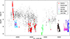 |
Fig. 1 Long-term activity of X Ser. Data from several databases were merged: DASCH, RoboScope (Honeycutt et al. 1998), the Catalina Survey, AAVSO, Duerbeck & Seitter (1990), Lick Obs. (Kinman et al. 1965). The short horizontal lines represent the upper limits of brightness if X Ser was not detected on the plate. The standard deviations of brightness are marked. The points were connected by a line in the densely covered parts of the light curves to guide the eye. See Sect. 3 for details. |
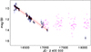 |
Fig. 2 Decaying branch of the classical nova outburst of X Ser (DASCH database). The standard deviations of brightness are shown. The short horizontal lines represent the upper limits of brightness. A linear fit of the decay and its standard deviation are also displayed (see Sect. 3 for details). |
3 Data analysis
3.1 Overview of the activity
Only one photographic observation of the DASCH field of X Ser was usually obtained per night. To ensure that the image of X Ser is not influenced by artifacts, the field of X Ser was inspected. This field, generated for the digitized DASCH plates, is a square with a field size of 20 arcmin with X Ser in its center.
The typical standard deviation of brightness of X Ser on the DASCH plates is about 0.2 mag (about 26% of the plates). This deviation is smaller than 0.4 mag on about 90% of the plates. We used only those plates where this deviation is less than 0.65 mag. The remaining five plates were therefore rejected.
A visual inspection of the light curve revealed that although X Ser was very bright in the DASCH plates of the nova outburst and this curve displayed a gradual decay in 1903, the SExtractor-based photometry also provided several upper limits of brightness that were several magnitudes deeper than the surrounding numerous detections. An inspection of these DASCH plates showed that X Ser was also very bright there, so we ascribed the non-detection by SExtractor to some instrumental effects (e.g., a distorted image of this object on the plate). A comparison of the light curve with the plates enabled us to remove these discrepancies.
Some CCD observations contain multiple detections of X Ser per night (sometimes several dozen). To make the light curves used for the analysis of the long-term activity and the histograms of brightness more uniform, the one-day means of brightness in CCD data were calculated.
The scatter of the AAVSO CCD photometry is often significantly larger in the faint state (V ~ 17), which we attribute to increased observational error as the star becomes fainter. An inspection of the light curves showed thatusing only the AAVSO CCD measurements with the quoted standard deviation of brightness of a single measurement smaller than 0.1 mag significantly diminished the noise and improved the light curves.
The listed standard deviations of brightness of the Catalina Real-time Transient Survey of X Ser in the V band were between 0.04 and 0.1 mag. A comparison of the AAVSO and Catalina CCD observations in their region of overlap showed the AAVSO data to be systematically 0.2 mag fainter. The AAVSO data were therefore adjusted by 0.2 mag to improve the agreement.
The time segment with the photographic observations (approximated as the B band) precedes that of the CCD V -band observing. It is true that we compare theB-band observations with those of the V -band, but the peak-to-peak amplitude of the brightness variations is several magnitudes, which is considerably larger than the possible changes of the color indices. The color variations are thus not expected to dramatically influence the large-amplitude light curve of X Ser in Fig.1.
The light curve of the classical nova outburst is displayed in Fig. 2. The upper limits of brightness of the pre-nova constrain the duration of this event. A linear fit and its standard deviation fulfill the profile of the decay. If this outburst was discovered close to its peak, then its t3 (the time neededto fall 3 mag below maximum) is about 526 days. Any part of the outburst with absent observations is at most 225 days.
The light curve of the post-nova X Ser was divided into several time segments to show its evolution (Fig. 3).
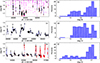 |
Fig. 3 Individual data sets of photometry of the post-nova X Ser. Panel a: photographic DASCH data (1932–1951). The events similar to those in Panel e are labeled 1 and 2. The short horizontal lines represent the upper limits of brightness. Panel b: histogram of brightness of the photographic data. Panel c: light curve from RoboScope (the V -band CCD data; 1992–1997; Honeycutt et al. 1998). The stunted outbursts are labeled H1, H2, and H3. Panel d: histogram of brightness of the RoboScope data. Panel e: light curve from Catalina Survey (2005–2013; circles) and CCD V -band AAVSO data (2009–2015; triangles). The outbursts investigated in Sect. 3.2 are labeled A to I. Panel f: histogram of brightness of the Catalina and AAVSO data (see Sect. 3 for details). |
3.2 Episodic brightenings (outbursts)
The detailed light curves of the individual, well observed brightenings (1, 2, E, F, G, H, I) are displayed in Fig. 4. The fits to those parts of the decaying branches that can be considered linear are included. The rising branch of outburst 1 is defined onlyby a single data point because of the gaps, but it is consistent with slow rises like the one in outburst H. Also, the rising branch of outburst 2 is hidden in the data gap, but its duration, constrained by the data points, is consistent with outburst H.
To investigate the shapes of the outbursts from Fig. 4, we shifted them along the time axis tomatch the decaying branch of the template. We selected only those outbursts (E, F, G, H, I) from Fig. 3g for the folding because their shapes (or at least their large parts) were well observed. Outburst F was chosen as the template because of its well-observed decaying branch. The brightness of 15.5 mag(V) was chosen as the reference level. The decaying branches of these outbursts are similar enough to each other that the quality of the match was to a large extent independent of the choice of the reference level.
The decaying branches of the individual outbursts were then merged into a common file and smoothed by the code HEC13, written by Prof. P. Harmanec. It is based on themethod of Vondrák (1969, 1977), who improved the original method of Whittaker & Robinson (1946). Figure 5 shows the result of the fitting.
Figure 3e shows a close similarity to the behavior of dwarf novae (DNe). We obtained an insight into the range of the recurrence times of these outbursts, TC, in the following way. The solid circles in Fig. 6a mark the times of the peaks of the observed outbursts. Each associated open circle represents the time elapsed between this outburst (marked by the solid circle and connected by a vertical line) and the time of the subsequent observed outburst. The uncertainty of the time of the peak of the outburst depends on the coverage by the data. Although this uncertainty can be about 15 d for some outbursts, it is considerably smaller than the length of TC.
A histogram of the time intervals between the observed outbursts in Fig. 6b shows a single broad bump with the peak at about 350 d; it indicates the most frequent outburst interval. The tail toward the longer TC can be at least partly caused by the gaps in the data and hence by the missed outbursts.
The decay rate τD is an important parameter of the light curves of the DN outbursts. The quantity τD is expressed in days for a decrease in brightness of 1 mag (Bailey 1975). A comparison of the outbursts of X Ser with those of DNe is shown in Fig. 7 where τD is plotted versus Porb. It enables us to assess how much a given outburst obeys the Bailey relation (Bailey 1975). The data come from Warner (1995); Shears & Poyner (2010); Šimon (2000a; DO Dra), and Šimon (2000b; DX And); the data for UY Pup were determined from the AAVSO database (Kafka 2017). It should be noted that the τD values of DO Dra and GK Per are lower than those of most DNe with comparable Porb. These two CVs are known to be the intermediate polars according to Patterson et al. (1992) and Watson et al. (1985).
The fit to the decaying branch of the ensemble of outbursts of X Ser from Fig. 5 shows that the outbursts of this CV obey the Bailey relation very well. For GK Per, only the steepest part of the decline was used for the determination of τD (see also Sect. 3.3).
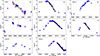 |
Fig. 4 Episodic brightenings (outbursts) of X Ser. Panels a and b: DASCH photographic light curves. The short horizontal lines represent the upper limits of brightness. Panel c: stunted outburst observed by Honeycutt et al. (1998). Panels d–i: CCD V -band AAVSO andCatalina data. The error bars of the AAVSO and Catalina data mark the standard deviation of the one-day mean of brightness. Solid lines mark the fits to those parts of the decaying branches that can be considered linear. The standard deviations of these fits are included. The scales of the horizontal axes are identical for all cases except outburst 2 (panel b). |
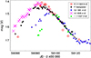 |
Fig. 5 Comparison of the outbursts in X Ser during the post-nova stage. The individual outbursts were shifted along the time axis to match the decaying branch of the template. The time of crossing 15.5 mag(V) and the time shifts with respect to the template are listed. The thick dashed curve represents the smoothed curve of the decaying branch. |
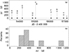 |
Fig. 6 Panel a: times of the observed outbursts in X Ser, marked in Fig. 3e,g. The horizontal line marksthe times of the outbursts (solid circles). The associated open circles denote the time between the specific outburst (marked by the solid circle) and the time elapsing to the subsequent observed outburst. Panel b: histogram of the times between the neighboring observed outbursts (see Sect. 3.2 for details). |
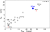 |
Fig. 7 Decayrate of DN outbursts, τD, versus Porb. Only DNe above the period gap (e.g., Warner 1995) are included. Crosses mark the intermediate polars. The data mostly come from Warner (1995) and Shears & Poyner (2010; see Sect. 3.2 for details). |
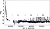 |
Fig. 8 Long-term activity of GK Per (AAVSO data Kafka 2016). The one-day means are used. After the return to quiescence from the classical nova outburst (1901), the initial nova-like activity was followed by a series of DN outbursts. The points represent the one-day means and were connected by a line in the densely observed parts of the light curves to guide the eye. The vertical lines mark the borders of three segments (S1, S2, S3; see Sect. 3.3 for details). |
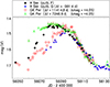 |
Fig. 9 Comparison of the representative outbursts of X Ser and GK Per in their post-nova stages. They are aligned according to their decaying branches. The outbursts of GK Per are shifted in time and brightness to match those of X Ser, as marked in the legend. A linear fit to the merged decaying branch of both outbursts of GK Per is included. See Sect. 3.2 for more. |
3.3 Comparison with the evolution of activity of GK Per
To comparethe time evolution of activity of X Ser with that of another CV with a very long Porb observed to have undergone a classical nova outburst, we plot the light curve of GK Per (Fig. 8). GK Per underwent this outburst in 1901, close in time to that of X Ser. GK Per displayed various types of activity in its post-nova stage (Hudec 1981; Sabbadin & Bianchini 1983).
We also compared the outbursts in the post-novae X Ser and GK Per (Fig. 9). The light curves of the DN outbursts inGK Per were adapted from the previous analysis (Šimon 2002). To avoid an overcrowding of the diagram, we included only two well-observed outbursts used in Šimon (2002). They are aligned according to their decaying branches.
4 Discussion
We show the strong long-term activity of the post-nova X Ser over a period of more than a hundred years when this system displayed the properties of various CV types.
The observed decay of this classical nova outburst is gradual, a large part of which is consistent with a linear decay in the magnitude scale. In variance with another type D nova, HR Del (Duerbeck 1981), any superimposed flares larger than the uncertainties of the measured brightnesses were missing. The classification as type D is thus based only on its very long time t3. The fact that the pre-nova X Ser was fainter than at the upper (brighter) end of all the post-nova histograms of brightness (Fig. 3) places constraints on a pre-nova gradual brightening in X Ser during the several years prior to its nova outburst, detected in some CVs by Robinson (1975) and Collazzi et al. (2009). The decay of the nova outburst in X Ser finished with the brightness, which is fainter than the peaks of the light curve of the post-nova (Fig. 3); this suggests that the complex brightness variations started shortly after the nova outburst.
The mutually similar faint ends of the histograms of brightness in Figs. 3b,d,f suggest that the luminosity of the post-nova X Ser was able to decrease to a relatively well defined brightness. The discrete outbursts of the post-nova X Ser in Fig. 3e bear a close similarity to the behavior of DNe, especially of the U Gem type (see, e.g., Warner 1995 for definition). The events in Figs. 3e and 4a,d,e,f,h show the mutually similar profiles, especially with regard to the decaying branches. The decay rate can be considered almost unchanged even for the events with considerably different peak magnitudes (Fig. 5). This suggests that all these decays are controlled by the same process with very similar parameters. The decay rate is consistent with the Bailey relation (Bailey 1975), appropriate for Porb of X Ser. This speaks in favor of a thermal-viscous instability of the disk. In this model, the decay is governed by propagation of cooling front (e.g., Smak 1984; Hameury et al. 1998). The slow rises of these events suggest that the outbursts of X Ser were always of the inside-out type. The different peak magnitudes of the individual outbursts can be explained if the radius of the ionized disk attained the different values.
The length of TC of about 270–320 d of the series of the DN outbursts of X Ser after JD 2 453 500 is similar to the periodicity of 275–277 d for the brightenings from about 16.5 mag to 14 mag mainly between 2 417 900 and 2 419 800 (Hughes Boyce 1942; Duerbeck & Seitter 1990). Generally, the TC of DNe are highly variable, but these variations are not random (e.g., Vogt 1980; Šimon 2002). The interpretation that some DN outbursts also occurred prior to the above-mentioned JD 2 453 500 is also supported by the decay rate of outburst 1 (Figs. 3a and 4a), consistent with that of the later DN outbursts shown in Figs. 3e,f.
According to Honeycutt et al. (1998) and Honeycutt (2001), an extra source of light could diminish the amplitude of the stunted outbursts in some CVs including X Ser. The width of the brighter bump in the histogram in Fig. 3d is caused by the gradual brightness variations, with only a minor contribution of the stunted outbursts. We also interpret outburst 2 (similar to the stunted outburst H1) in Fig. 3a as a stunted outburst because of its peculiar decay; it was halted for more than 30 days after a decline by about 1 mag from the peak (the value consistent with other stunted outbursts). We argue that this extra source of light would have to form rapidly in X Ser because outburst 2 started from a brightness value that was consistent with a quiescence value that is usual for the later series of the DN outbursts (see Fig. 3e). This places constraints on the extra emitting source; it appeared during a DN outburst which started from a usual quiescence level.
Honeycutt (2001) argue that there is a correlation between the presence of stunted outbursts and the time that has elapsed since the classical nova explosion. In this regard we show that in variance with the stunted outbursts of X Ser observed by Honeycutt et al. (1998) and Honeycutt (2001; Fig. 3c), the later outbursts in Fig. 3e start from a considerably fainter brightness, and their amplitudes and durations are larger. We therefore argue that the stunted outbursts did not occur in X Ser after JD 2 453 500 because the whole disk was in the cool state between the DN outbursts.
We explain the scatter of the Bailey relation of X Ser and GK Per, which have similar, very long Porb, by the fact that GK Per is the intermediate polar, so its inner disk region is truncated by the magnetic field of the WD (Warner 1995). In the model of Cannizzo (1994), this leads to a decrease of τD.
The time evolution of the activity of the post-nova GK Per can be explained if the inner disk region remained in the ionized state due to irradiation by the hot, slowly cooling WD, while a thermal-viscous instability could already occur in the outer disk region, as modeled by Schreiber et al. (2000) and Mineshige et al. (1990). However, the occasional bright states of the post-nova X Ser, which give rise to the broad brighter peaks in the histograms in Fig. 3b,d, can hardly be attributed to the role of the WD cooling down after the nova outburst. Occasional increases in the mass outflow from the donor star toward the disk are a more viable explanation.
The time evolution of activity of a post-nova with the accretion disk appears to depend on its Porb. Shara et al. (2007, 2012) found a nova shell of Z Cam (Porb = 0.289840 d; Kraft et al. 1969) whose nova outburst took place 220–2 000 years ago, and concluded that at least some classical novae become DNe long after their nova thermonuclear outbursts. Shara et al. (2017) show that another Z Cam system, AT Cnc (Porb = 0.2011 d; Nogami et al. 1999), underwent a nova outburst even only 330 yr ago. BK Lyn with Porb = 107.97 min (Ringwald et al. 1996), associated with Nova Lyncis 101 (Ho 1962; Hertzog 1986), transitioned to the ER UMa type DN from a nova-like display after2000 years (Patterson et al. 2013). We emphasize that the post-novae X Ser and GK Per (along with V1017 Sgr = Nova Sgr 1919; Porb = 5.786 d; McLaughlin & Dean 1946; Sekiguchi 1992; Salazar et al. 2017), i.e., the systems with Porb exceptionally long for CVs (hence with the large disks), displayed the DN outbursts over less than a century after the nova outburst.
5 Conclusion
This analysis shows that the activity of the post-nova X Ser displays both DN and nova-like features. The decaying branches of most of these DN outbursts obey the Bailey law for outbursts of DNe. The occurrence of the DN outbursts shortly after the end of the classical nova outburst of X Ser thus suggests that the mass transfer rate into the disk was usually not sufficiently high to prevent a thermal-viscous instability in the post-nova stage.
Acknowledgements
Support by grant 13-33324S of the Grant Agency of the Czech Republic is acknowledged. This work was supported by the project RVO:67985815. I also acknowledge The DASCH project at Harvard, partially supported from NSF grants AST-0407380, AST-0909073, and AST-1313370. This research has also made use of the observations from the AAVSO International database (USA) and the Catalina Transient Survey. I thank the variable star observers worldwide. I also thank Prof. Petr Harmanec for providing me with the code HEC13. The Fortran source version, compiled version, and brief instructions on how to use the program can be obtained at this site: http://astro.troja.mff.cuni.cz/ftp/hec/HEC13/
References
- Bailey, J. 1975, J. Br. Astr. Ass., 86, 30 [Google Scholar]
- Cannizzo, J. K. 1994, ApJ, 435, 389 [NASA ADS] [CrossRef] [Google Scholar]
- Collazzi, A. C., Schaefer, B. E., Xiao, L., et al. 2009, AJ, 138, 1846 [NASA ADS] [CrossRef] [Google Scholar]
- Cordova, F. A., Jensen, K. A., & Nugent, J. J. 1981, MNRAS, 196, 1 [NASA ADS] [CrossRef] [Google Scholar]
- Crampton, D., Cowley, A. P., & Fisher, W. A. 1986, ApJ, 300, 788 [NASA ADS] [CrossRef] [Google Scholar]
- Drake, A. J., Djorgovski, S. G., Mahabal, A., et al. 2009, ApJ, 696, 870 [NASA ADS] [CrossRef] [MathSciNet] [Google Scholar]
- Duerbeck, H. W. 1981, PASP, 93, 165 [NASA ADS] [CrossRef] [Google Scholar]
- Duerbeck, H. W. 1987, Space Sci. Rev., 45, 1 [NASA ADS] [CrossRef] [Google Scholar]
- Duerbeck, H. W., & Seitter, W. C. 1990, in IAU Colloq. 122: Physics of Classical Novae, eds. A. Cassatella, & R. Viotti (Berlin: Springer Verlag), Lect. Notes Phys., 369, 165 [CrossRef] [Google Scholar]
- Grindlay, J. E., & Griffin, R. E. 2012, IAU Symp., 285, 243 [Google Scholar]
- Grindlay, J., Tang, S., Los, E., et al. 2012, IAU Symp., 285, 29 [Google Scholar]
- Hameury, J.-M., Menou, K., Dubus, G., et al. 1998, MNRAS, 298, 1048 [NASA ADS] [CrossRef] [Google Scholar]
- Hertzog, K. P. 1986, The Observatory, 106, 38 [Google Scholar]
- Ho, P. Y. 1962, Vistas Astron., 5, 127 [CrossRef] [Google Scholar]
- Honeycutt, R. K. 2001, PASP, 113, 473 [NASA ADS] [CrossRef] [Google Scholar]
- Honeycutt, R. K., Robertson, J. W., & Turner, G. W. 1998, AJ, 115, 2527 [NASA ADS] [CrossRef] [Google Scholar]
- Hudec, R. 1981, Bull. Astron. Inst. Czechosl., 32, 93 [NASA ADS] [Google Scholar]
- Hughes Boyce,E. 1942, Harv. Ann., 109, 10 [Google Scholar]
- Kafka, S. 2016, Observations from the AAVSO International Database, http://www.aavso.org [Google Scholar]
- Kafka, S. 2017, Observations from the AAVSO International Database, http://www.aavso.org [Google Scholar]
- Kinman, T. D., Wirtanen, C. A., & Janes, K. A. 1965, ApJS, 11, 223 [CrossRef] [Google Scholar]
- Kraft, R. P., Krzeminski, W., & Mumford, G. S. 1969, ApJ, 158, 589 [NASA ADS] [CrossRef] [Google Scholar]
- Leavitt, H. 1908, Harv. Circ., 142 [Google Scholar]
- McLaughlin, & Dean, B. 1946, PASP, 58, 46 [CrossRef] [Google Scholar]
- Mineshige, S., Tuchman, Y., & Wheeler, J. C. 1990, ApJ, 359, 176 [NASA ADS] [CrossRef] [Google Scholar]
- Nogami, D., Masuda, S., Kato, T., et al. 1999, PASJ, 51, 115 [NASA ADS] [CrossRef] [Google Scholar]
- Patterson, J., Schwartz, D. A., Pye, J. P., et al. 1992, ApJ, 392, 233 [NASA ADS] [CrossRef] [Google Scholar]
- Patterson, J., Uthas, H., Kemp, J., et al. 2013, MNRAS, 434, 1902 [NASA ADS] [CrossRef] [Google Scholar]
- Ringwald, F. A., Naylor, T., & Mukai, K. 1996, MNRAS, 281, 192 [NASA ADS] [Google Scholar]
- Robinson, E. L. 1975, AJ, 80, 515 [NASA ADS] [CrossRef] [Google Scholar]
- Sabbadin, F., & Bianchini, A. 1983, A&AS, 54, 393 [NASA ADS] [Google Scholar]
- Salazar, I. V., LeBleu, A., Schaefer, B. E., et al. 2017, MNRAS, 469, 4116 [NASA ADS] [CrossRef] [Google Scholar]
- Schreiber, M. R., Gänsicke, B. T., & Cannizzo, J. K. 2000, A&A, 362, 268 [NASA ADS] [Google Scholar]
- Sekiguchi, K. 1992, Nature, 358, 563 [NASA ADS] [CrossRef] [Google Scholar]
- Shara, M. M., Martin, C. D., Seibert, M., et al. 2007, Nature, 446, 159 [NASA ADS] [CrossRef] [Google Scholar]
- Shara, M. M., Mizusawa, T., Zurek, D., et al. 2012, ApJ, 756, 107 [NASA ADS] [CrossRef] [Google Scholar]
- Shara, M. M., Drissen, L., Martin, T., et al. 2017, MNRAS, 465, 739 [NASA ADS] [CrossRef] [Google Scholar]
- Shears, J., & Poyner, G. 2010, JBAA, 120, 169 [NASA ADS] [Google Scholar]
- Šimon, V. 2000a, A&A, 360, 627 [NASA ADS] [Google Scholar]
- Šimon, V. 2000b, A&A, 364, 694 [NASA ADS] [Google Scholar]
- Šimon, V. 2002, A&A, 382, 910 [NASA ADS] [CrossRef] [EDP Sciences] [Google Scholar]
- Šimon, V. 2017a, Frontier Research in Astrophysics – II, Proc. Sci., 269, 46 [NASA ADS] [Google Scholar]
- Šimon, V. 2017b, The Golden Age of Cataclysmic Variables and Related Objects – IV, Proc. Sci., 315, 35 [Google Scholar]
- Smak, J. 1984, Acta Astron., 34, 161 [NASA ADS] [Google Scholar]
- Thorstensen, J. R., & Taylor, C. J. 2000, MNRAS, 312, 629 [NASA ADS] [CrossRef] [Google Scholar]
- Vogt, N. 1980, A&A, 88, 66 [NASA ADS] [Google Scholar]
- Vondrák, J. 1969, Bull. Astron. Inst. Czechosl., 20, 349 [NASA ADS] [Google Scholar]
- Vondrák, J. 1977, Bull. Astron. Inst. Czechosl., 28, 84 [NASA ADS] [Google Scholar]
- Walker, A. D. 1923, Harv. Ann., 84, 198 [Google Scholar]
- Warner, B. 1995, Cataclysmic Variable Stars (Cambridge, UK: Cambridge University Press) [CrossRef] [Google Scholar]
- Watson, M. G., King, A. R., & Osborne, J. 1985, MNRAS, 212, 917 [NASA ADS] [CrossRef] [Google Scholar]
- Whittaker, E.,& Robinson, G. 1946, The Calculus of Observations (London: Blackie & Son), 303 [Google Scholar]
- Williams, G. 1983, ApJS, 53, 523 [NASA ADS] [CrossRef] [Google Scholar]
All Figures
|
Fig. 1 Long-term activity of X Ser. Data from several databases were merged: DASCH, RoboScope (Honeycutt et al. 1998), the Catalina Survey, AAVSO, Duerbeck & Seitter (1990), Lick Obs. (Kinman et al. 1965). The short horizontal lines represent the upper limits of brightness if X Ser was not detected on the plate. The standard deviations of brightness are marked. The points were connected by a line in the densely covered parts of the light curves to guide the eye. See Sect. 3 for details. |
| In the text | |
|
Fig. 2 Decaying branch of the classical nova outburst of X Ser (DASCH database). The standard deviations of brightness are shown. The short horizontal lines represent the upper limits of brightness. A linear fit of the decay and its standard deviation are also displayed (see Sect. 3 for details). |
| In the text | |
|
Fig. 3 Individual data sets of photometry of the post-nova X Ser. Panel a: photographic DASCH data (1932–1951). The events similar to those in Panel e are labeled 1 and 2. The short horizontal lines represent the upper limits of brightness. Panel b: histogram of brightness of the photographic data. Panel c: light curve from RoboScope (the V -band CCD data; 1992–1997; Honeycutt et al. 1998). The stunted outbursts are labeled H1, H2, and H3. Panel d: histogram of brightness of the RoboScope data. Panel e: light curve from Catalina Survey (2005–2013; circles) and CCD V -band AAVSO data (2009–2015; triangles). The outbursts investigated in Sect. 3.2 are labeled A to I. Panel f: histogram of brightness of the Catalina and AAVSO data (see Sect. 3 for details). |
| In the text | |
|
Fig. 4 Episodic brightenings (outbursts) of X Ser. Panels a and b: DASCH photographic light curves. The short horizontal lines represent the upper limits of brightness. Panel c: stunted outburst observed by Honeycutt et al. (1998). Panels d–i: CCD V -band AAVSO andCatalina data. The error bars of the AAVSO and Catalina data mark the standard deviation of the one-day mean of brightness. Solid lines mark the fits to those parts of the decaying branches that can be considered linear. The standard deviations of these fits are included. The scales of the horizontal axes are identical for all cases except outburst 2 (panel b). |
| In the text | |
|
Fig. 5 Comparison of the outbursts in X Ser during the post-nova stage. The individual outbursts were shifted along the time axis to match the decaying branch of the template. The time of crossing 15.5 mag(V) and the time shifts with respect to the template are listed. The thick dashed curve represents the smoothed curve of the decaying branch. |
| In the text | |
|
Fig. 6 Panel a: times of the observed outbursts in X Ser, marked in Fig. 3e,g. The horizontal line marksthe times of the outbursts (solid circles). The associated open circles denote the time between the specific outburst (marked by the solid circle) and the time elapsing to the subsequent observed outburst. Panel b: histogram of the times between the neighboring observed outbursts (see Sect. 3.2 for details). |
| In the text | |
|
Fig. 7 Decayrate of DN outbursts, τD, versus Porb. Only DNe above the period gap (e.g., Warner 1995) are included. Crosses mark the intermediate polars. The data mostly come from Warner (1995) and Shears & Poyner (2010; see Sect. 3.2 for details). |
| In the text | |
|
Fig. 8 Long-term activity of GK Per (AAVSO data Kafka 2016). The one-day means are used. After the return to quiescence from the classical nova outburst (1901), the initial nova-like activity was followed by a series of DN outbursts. The points represent the one-day means and were connected by a line in the densely observed parts of the light curves to guide the eye. The vertical lines mark the borders of three segments (S1, S2, S3; see Sect. 3.3 for details). |
| In the text | |
|
Fig. 9 Comparison of the representative outbursts of X Ser and GK Per in their post-nova stages. They are aligned according to their decaying branches. The outbursts of GK Per are shifted in time and brightness to match those of X Ser, as marked in the legend. A linear fit to the merged decaying branch of both outbursts of GK Per is included. See Sect. 3.2 for more. |
| In the text | |
Current usage metrics show cumulative count of Article Views (full-text article views including HTML views, PDF and ePub downloads, according to the available data) and Abstracts Views on Vision4Press platform.
Data correspond to usage on the plateform after 2015. The current usage metrics is available 48-96 hours after online publication and is updated daily on week days.
Initial download of the metrics may take a while.