| Issue |
A&A
Volume 614, June 2018
|
|
|---|---|---|
| Article Number | A16 | |
| Number of page(s) | 19 | |
| Section | Planets and planetary systems | |
| DOI | https://doi.org/10.1051/0004-6361/201630136 | |
| Published online | 07 June 2018 | |
Direct imaging of an ultracool substellar companion to the exoplanet host star HD 4113 A★
1
Département d’Astronomie, Université de Genève, 51 chemin des Maillettes,
1290
Versoix,
Switzerland
e-mail: This email address is being protected from spambots. You need JavaScript enabled to view it.
2
Université Grenoble Alpes, CNRS, IPAG,
38000
Grenoble,
France
3
Institute for Astronomy, University of Hawai’i,
2680 Woodlawn Drive,
Honolulu,
HI
96822,
USA
Received:
25
November
2016
Accepted:
18
December
2017
Abstract
Using high-contrast imaging with the SPHERE instrument at the Very Large Telescope (VLT), we report the first images of a cold brown dwarf companion to the exoplanet host star HD 4113A. The brown dwarf HD 4113C is part of a complex dynamical system consisting of a giant planet, a stellar host, and a known wide M-dwarf companion. Its separation of 535 ± 3 mas and H-band contrast of 13.35 ± 0.10 mag correspond to a projected separation of 22 AU and an isochronal mass estimate of 36 ± 5 MJ based on COND models. The companion shows strong methane absorption, and through fitting an atmosphere model, we estimate a surface gravity of logg = 5 and an effective temperature of ~500–600 K. A comparison of its spectrum with observed T dwarfs indicates a late-T spectral type, with a T9 object providing the best match. By combining the observed astrometry from the imaging data with 27 years of radial velocities, we use orbital fitting to constrain its orbital and physical parameters, as well as update those of the planet HD 4113A b, discovered by previous radial velocity measurements. The data suggest a dynamical mass of 66−4+5 MJ and moderate eccentricity of 0.44−0.07+0.08 for the brown dwarf. This mass estimate appears to contradict the isochronal estimate and that of objects with similar temperatures, which may be caused by the newly detected object being an unresolved binary brown dwarf system or the presence of an additional object in the system. Through dynamical simulations, we show that the planet may undergo strong Lidov-Kozai cycles, raising the possibility that it formed on a quasi-circular orbit and gained its currently observed high eccentricity (e ~ 0.9) through interactions with the brown dwarf. Follow-up observations combining radial velocities, direct imaging, and Gaia astrometry will be crucial to precisely constrain the dynamical mass of the brown dwarf and allow for an in-depth comparison with evolutionary and atmosphere models.
Key words: planets and satellites: detection / planet-star interactions / brown dwarfs
Based on observations collected at the European Organisation for Astronomical Research in the Southern Hemisphere under ESO programmes 097.C-0893(A), 077.C-0293(A), 279.C-5052(A), 081.C-0653(A) and 091.C-0721(B).
© ESO 2018
1 Introduction
The nearby G5 dwarf HD 4113A hosts a giant planet with one of the highest known orbital eccentricities (e = 0.9). The planetary companion, HD 4113A b, was first detected through radial velocity (RV) measurements by Tamuz et al. (2008) using the CORALIE spectrograph on the 1.2 m Swiss telescope at La Silla Observatory, as part of a planet search survey of a well-defined sample of solar-type stars (Udry et al. 2000).
Such a high eccentricity is commonly explained through Lidov-Kozai (Kozai 1962; Lidov 1962) interactions with a companion on a wider orbit, among other possible reasons. The RV measurements presented by Tamuz et al. (2008) also revealed a long-term trend, indicative of such a companion with a much longer orbital period. These data suggested a minimum mass of 10 MJ and minimum semi-major axis of 8 AU. Using this knowledge, we made several unsuccessful attempts to image this companion, first, with the NACO instrument at the VLT, using H-band spectral differential imaging (Smith 1987, SDI) in 2006 and 2007 (Montagnier 2008), coronagraphy in 2008 and non-coronagraphic L-band ADI in 2013 (Hagelberg 2014). A summary of the L-band ADI results is presented in Appendix A. These observations ruled out stellar companions between 0.2–2.5 arcsec (8–100 AU), suggesting that the outer companion was a brown dwarf.
In addition, a comoving stellar companion to HD 4113A was discovered by Mugrauer et al. (2014) at a much larger separation (49 arcsec, 2000 AU) and was identified as an early-M dwarf using near-IR photometry. The low mass of HD 4113B and its extremely long period cannot explain the observed RV drift. The authors also excluded the presence of any additional stellar companions between 190 and 6500 AU down to the hydrogen-burning mass limit.
While these previous imaging observations significantly narrowed down the parameter space in which to detect the unseen companion, the most recent generation of extreme adaptive optics (AO) instruments such as SPHERE (Beuzit et al. 2008) and GPI (Macintosh et al. 2008) are able to obtain higher contrasts at smaller angular separations, opening the search to even lower masses.
We herereport the first direct images of the suspected companion HD 4113C, confirming its presumed nature as that of a brown dwarf. In addition, we extend the time baseline of the RV observations by six years. When combined with the imaging data, this allows constraints to be placed on the mass and orbital parameters of the brown dwarf and planetary companion.
The paper is organized as follows: in Sect. 2 we revisit the stellar parameters of HD 4113A+B, using the most recent available data to better constrain the mass and age of the host and the dwarf. In Sect. 3 we summarize the observationsand data analysis procedures for the RV and high-contrast imaging data. In Sect. 4 we present the results of the imaging data analysis and derived companion properties, give an overview of the results from the combined orbital fitting, and report the results of dynamical simulations showing the interactions between the brown dwarf and giant planet. We conclude in Sect. 5 with a summary of our results and their implications.
2 Stellar parameters
Following the recent Gaia Data Release 1 (Gaia Collaboration et al. 2016), we are able to refine the stellar parameters of HD 4113A+B. These data give an improved parallax of π = 24.0 ± 0.2 mas, setting the star at a slightly closer distance to the Sun than previously thought (d = 41.7 ± 0.7 pc). A systematic error of 0.4312 mas – corresponding to the astrometric excess noise measured by Gaia – was quadratically added to the parallax error to absorb a suspected bias linked to the signature of HD 4113A b in the Gaia data.
For HD 4113A, we combined the Gaia parallaxes with the hipparcos and 2MASS photometry (Skrutskie et al. 2006) to derive the absolute magnitudes listed in Table 1. Teff, log g, and [Fe/H] were taken from the spectroscopic analysis reported by Tamuz et al. (2008), while the v sini and the  were derived from the CORALIE-07 spectra following the approach of Santos et al. (2002) and Lovis et al. (2011) that are implemented in CORALIE by Marmier (2014). The fundamental parameters of this metal-rich star ([Fe/H] = 0.20 ± 0.04) were derived using the Geneva stellar evolution models (Mowlavi et al. 2012). The interpolation in the model grid was made through a Bayesian formalism using observational Gaussian priors on Teff, MV, log g, and [Fe/H] (Marmier 2014). We derived a mass of
  and an age of
  Gyr.
Gyr.
While HD 4113B is likely to have similar metal enrichment as HD 4113A, Delfosse et al. (2000) showed that the mass-luminosity relation for M dwarfs in the near-infrared is only marginally affected by metallicity. For this reason, we used the solar metallicity model grids of Baraffe et al. (2015) combined with the 2MASS and Sofi/ESO NTT near-infrared photometry (Mugrauer et al. 2014) to derive its stellar parameters. The interpolation in the model grid was made through a Bayesian formalism using observational Gaussian priors on MJ, MH, MK, and the H − K color index. Through this approach, we obtain a stellar mass of MB = 0.55M⊙ and an effective temperature of Teff = 3833 K, in agreement with an M0-1V spectral type (Rajpurohit et al. 2013). All observed and derived stellar parameters are given in Table 1.
Stellar parameters of HD 4113 A and B
3 Observations and data reduction
3.1 Radial velocities
Since the discovery of HD 4113A b by Tamuz et al. (2008), we have acquired more than 166 additional RV measurements of HD 4113A, with the goal of better characterizing the long period and more massive companion responsible for the observed RV drift. The 272 measurements obtained between October 1999 and September 2017 are shown in Fig. 1 with the corresponding Keplerian model for HD 4113A b and the long-term drift. During that period of time, CORALIE underwent two upgrades that introduced small zero-point RV offsets (Ségransan et al. 2010). To account for these, we considered the data as originating from three different instruments with unknown offsets: CORALIE-98, CORALIE-07, and CORALIE-14. These values were then included in the orbital fit as additional parameters. We also included 16 KECK-HIRES RV measurements (Butler et al. 2017) covering a 10-year time span from 2004 to 2014. Four unpublished measurements from the CORAVEL spectrograph taken between May 1989 and July 1994 were also added. While these measurements have large uncertainties, the significant increase in time baseline helps to constrain the possible amplitude and period of the signal introduced by the long-period companion responsible for the RV drift. Owing to their large error bars, CORAVEL measurements are only shown in the bottom panel of Fig. 1.
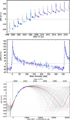 |
Fig. 1 Radial velocity measurements of HD 4113A taken with CORALIE (blue dots for data taken before the 2007 upgrade, and purple dots for data taken later) and with HIRES (orange dots), covering the time period from October 1999 to September 2017. Four CORAVEL measurements from as early as May 1989 are also included (black dots), extending the time baseline to 28 years. The top panel represents the observed CORALIE RV time series with the eccentric-orbit model of thegiant planet HD 4113A b as well as the long-term drift corresponding to HD 4113 C. The middle panel shows a phase-folded representation of the RV orbit of HD 4113A b, while the bottom panel shows the predicted and observed RVs for the orbit of HD 4113C after subtracting the signal produced by HD 4113A b. Several possible orbits drawn from the output of our MCMC procedure are shown. The bold red curve represents the maximum likelihood solution. |
3.2 2016 SPHERE high-contrast imaging
The source HD 4113A was observed with SPHERE, the extreme AO system at the VLT (Beuzit et al. 2008) on 2016-07-20 (Program 097.C-0893, PI Cheetham). Observations were taken in IRDIFS mode, which allows the Integral Field Spectrograph (IFS; Mesa et al. 2015) and InfraRed Dual-band Imager and Spectrograph (IRDIS; Dohlen et al. 2008) modules to be used simultaneously. The IFS data cover a range of wavelengths from 0.96–1.34 μm with an average spectral resolution of 55.1. The IRDIS data were taken in the dual-band imaging mode (Vigan et al. 2010) using the H2 and H3 filters ( m,
m, 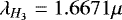 m), designed such that the H3 filter aligns with a methane absorption band. The conditions during the observations were good, with stable wind and seeing, but with some intermittent clouds that may affect the photometry.
The observing sequence consisted of long-exposure images taken with an apodized Lyot coronagraph (Soummer et al. 2003) with a spot diameter of 185 mas. To measure the position of the star behind the coronagraph, several exposures were taken with a sinusoidal modulation applied to the deformable mirror (to generate satellite spots around the star) at the beginning and end of the sequence. To estimate the stellar flux and the shape of the point-spread function (PSF) during the sequence, several short-exposure images were taken with the star moved from behind the coronagraph and using a neutral-density filter with a ~10% transmission, also at the beginning and end of the sequence. In addition, several long-exposure sky frames were taken to estimate the background flux and help identify bad pixels on the detector. The observing sequence included a maximum of 54 deg of field rotation between the coronagraphic frames. The observing parameters are given in Table 2.
The SPHERE Data Reduction and Handling pipeline (Pavlov et al. 2008, v0.18.0) was used to perform the wavelength extraction for the IFS data, turning the full-frame images of the lenslet spectra into image cubes.
The remainder of the data reduction and analysis procedure was completed using the GRAPHIC pipeline (Hagelberg et al. 2016), with recent modifications to handle SPHERE data. The data were first sky subtracted, flat fielded, cleaned of bad pixels, and corrected for distortion (following Maire et al. 2016). The position of the primary star was measured from the images with the satellite spots, and the average value was used as the assumed position. The measured difference between the values measured atthe start and end of the sequence was 2.5 mas. Coronagraphic images were then shifted to the measured center position using Fourier transforms.
An implementation of the principal component analysis (PCA) PSF subtraction algorithm (Soummer et al. 2012) was then run separately for images at each wavelength and for each IRDIS channel. The resulting frames were derotated and median combined toproduce a final PSF-subtracted image. The PCA algorithm was applied separately to annular sections of each image. Each annulus had a width of 2 FWHM (calculated for each channel individually). One annulus was centered on the observed position of the companion, and the remaining annuli were defined inwards and outwards until reaching theedge of the coronagraph and the edge of the field of view. To minimize companion self-subtraction, we excluded images with small changes in parallactic angle when building a reference library for each image and annulus. Our chosen criteria required that a companion in the center of each annulus would move by no less than 1.25× the PSF FWHM due to sky rotation.
The PCA-reduced IRDIS and IFS images are shown in Fig. 2 for reductions removing 20 PCA modes. We clearly detect a companion, which we refer to as HD 4113C, and use its observed position to optimize and inform the remaining data analysis steps.
An additional SDI reduction was performed for both the IFS and IRDIS datasets. For IRDIS, the images in the H3 filter were rescaled by the ratio of the wavelengths using Fourier transforms, and subtracted from the H2 images taken simultaneously. As a result of instrumental throughput and stellar flux differences between the two channels, the values in the H3 images were scaled to have the same total flux in an annular region of the speckle halo centered on the edge of the AO-correction radius. The same PCA algorithm was then performed on the resulting images.
For each IFS image, the corresponding images in other wavelength channels were rescaled by the ratio of the wavelengths and flux-scaled using the same approach used for IRDIS. A PSF reference was constructed from the median of these rescaled images and subtracted from the original image. Based on the known position of the brown dwarf from the IRDIS reduction, only wavelength channels where the companion position was shifted by 1.5 FWHM or more were considered to minimize self-subtraction. This was repeated for each image at each wavelength, before applying PCA.
An estimation of the noise as a function of radius from the star was obtained from the standard deviation of the pixel values measured in an annulus of width λ∕D. The location of HD 4113C was masked out for this calculation to avoid biasing the measurements. This was then converted into a contrast curve accounting for the throughput of the PCA reduction and small sample statistics (following the approach of Mawet et al. 2014). The 5 σ contrast curves obtained through this method are shown in Fig 3.
The position and relative flux of HD 4113C were measured from the IRDIS data by subtracting a shifted and flux-scaled copy of the observed PSF of HD 4113A from the final combined image. The PSF was obtained using the mean of the unobscured images of HD 4113A taken with the ND filter. The separation, position angle, and flux of the subtracted PSF were varied to minimize the residuals in a small (3λ∕D) area. This was achieved using a nonlinear least-squares optimizer. A true-north offset of − 1.75 ± 0.08 deg and a plate scale of 12.255 ± 0.009 mas/pix were used to calculate the separation and position angle of the companion, using the measurements presented in Maire et al. (2016). We also adopt a systematic uncertainty in the star position of ± 3 mas.
To estimate the uncertainties on the fitted position and flux, we applied a bootstrapping procedure. The PCA-subtracted and derotated frames were saved before stacking to generate a final image. We resampled the data (with replacement) to generate 1000 sets of frames, with each set having the same number of frames as the original data. These were collapsed to give 1000 final images. The fitting process described above was then performed on each, giving a distribution of values for the separation, position angle, and contrast. The mean and standard deviation of these distributions were used as an estimate of the parameter values and their uncertainties.
As an additional measure, this procedure was then repeated for a range of PCA reductions by varying the number of modes, protection angle, and annulus width. The scatter between the mean values for each reduction were included in our listed uncertainties.
For the IFS data, a different approach was taken to measure the companion flux because of the low signal-to-noise ratio (S/N) or non-detection of HD 4113C in many spectral channels. The position of the companion was fixed to that measured from the stacked image, and a fit was performed to the flux alone. The uncertainty was estimated by performing the same procedure at positions both in a ring with a radius of 2 FWHM around HD 4113C and at a range of position angles at the same separation. The scatter of these values was taken as the uncertainty.
Observing log for the two SPHERE datasets.
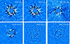 |
Fig. 2 PSF-subtracted images from each dataset and epoch. For the 2016 dataset, the IRDIS H2, H3, and SDI (H2-H3) reductions are shown, while we show only the 2015 IRDIS SDI (K1-K2) reduction. We also show a weighted combination of the IFS SDI images for each epoch. Each IFS wavelength channel was weighted by the average flux predicted by the best-fitting Morley et al. (2012) and Tremblin et al. (2015) models. The strong detection of the companion in H2 and the lack of a H3 counterpart indicates the presence of strong methane absorption. All images have the same scale and orientation, and were generated by removing 20 PCA modes. |
3.3 Archival SPHERE data
We also re-reduced the SPHERE observations of HD 4113 published in Moutou et al. (2017) (Program 096.C-0249, PI: Moutou), taken on 2015-10-08. These observations were taken in IRDIFS-EXT mode following an observing strategy that is similar to our observationsas described above, and are summarized in Table 2. The IRDIS data were taken in the K1-K2 mode (λK1 = 2.1025μm, λK2 = 2.2255μm), while the IFS data cover a range of wavelengths from 0.97–1.66 μm with an average spectral resolution of 34.5. These data include a maximum field rotation of 51 deg between coronagraphic frames.
Our data reduction procedure was identical to that of the IRDIFS data described in the previous section.
4 Results
4.1 SPHERE 2016 high-contrast imaging data
The source HD 4113C was detected at high significance in both IRDIS H2 and IRDIS SDI reductions, but was not recovered in the H3 filter, suggesting the presence of strong methane absorption. The measured relative photometry and astrometry are given in Table 3, while the IRDIS PSF-subtracted images are shown in Fig. 2. We adopt a lower limit on the contrast of 14.8 mag for the H3 filter, using the 3 σ contrast curve at the location of the H2 detection.
In the IFS data using PCA alone, no significant detection was found in any individual wavelength channel or in the mean taken over wavelength.
After we applied SDI to the IFS data, we clearly detected the companion, with 14 of the wavelength channels showing an excess of flux above 1.5 σ significance at the location of the IRDIS detection. A weighted-mean image is shown in Fig. 2. The data reduction for wavelengths below 1.02μm suffer from considerably more residual noise in the SDI+PCA reduction and are not included in the subsequent analysis.
The measured contrast ratios from IFS and IRDIS were converted into apparent flux measurements through multiplication by a BT-NextGen spectral model (Allard et al. 2012) with Teff = 5700 K, [Fe/H] = 0.3 dex and logg = 4.5, close to the values determined in Sect. 2. The model spectrum was flux-scaled using the distance and radius of HD 4113A. The extracted spectrum is shown in Fig. 4.
Measured astrometry and photometry of HD 4113C from the SPHERE observations.
4.2 SPHERE archival high-contrast imaging data
After processing the 2015 data, we were unable to unambiguously recover the companion HD 4113C in the IRDIS images. Close to the location of the 2016 detection, we find an excess of flux with 2–3 σ significance in the SDI reduction. However, because of the lower S/N, our reduction of the IRDIS data does not provide substantial constraints on the position or flux of the companion, and we have excluded it from the following analysis.
In the IFS SDI reduction, we also find an excess of flux in wavelength channels corresponding to the J- and H-band peaks found in the2016 data, again with lower significance. We find six channels at which the companion is visible at S∕N > 4, and by combining the final images with knowledge of the measured spectrum from the 2016 data, we obtain a detection with S∕N > 5. From this image, we were able to calculate the position of HD 4113C listed in Table 3. Because of the lower S/N, we did not include the flux measurements in our analysis of the companion.
The difference in the observed position between the two epochs demonstrates orbital motion at the 3 σ level. The observed motion also differs strongly from that expected by a background object because of the 125 mas yr−1 proper motion of HD 4113, demonstrating that it is indeed comoving.
The detection limits obtained from the IRDIS data are shown in Fig. 3. Our IFS reduction produces contrast limits similar to those reported in Moutou et al. (2017).
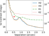 |
Fig. 3 5 σ contrast obtained for the four IRDIS datasets (K1 and K2 from the 2015 data, and H2 and H3 from the 2016 data). The measured separation and contrast of the companion detected in the H2 band is marked in red. |
4.3 Companion properties
To allow a consistent comparison with other objects and to estimate the mass of HD 4113C, we converted the H2 flux into an absolute magnitude using the distance of HD 4113 from Table 1.
In addition to the H2 measurement, we used the IFS spectrum to calculate a synthetic J-band magnitude for HD 4113C using a top-hat function between 1.125–1.365 μm. For both the J and H2 filters, we used the calibrated spectrum of Vega from Bohlin (2007) to calculate the flux corresponding to zero magnitude. The resulting absolute photometric magnitudes are listed in Table 4.
The measured absolute photometry can then be compared with substellar evolutionary models. We used the COND (Baraffe et al. 2003)substellar isochrones to predict the companion photometry as a function of age, temperature, and mass in each band. We then interpolated this grid to estimate the parameters of HD 4113C.
The measured H2 magnitude MH2 = 16.6 ± 0.1 corresponds to a mass of 36 ± 5 MJ. The isochrones predict a temperature of 690 ± 20 K and an H3 contrast of 14.9 mag, which is close to our lower limit of 14.8 mag. The J-band magnitude MJ = 18.5 ± 0.2 leads to estimates of 29 ± 5 MJ and 580 ± 20 K. However, few benchmark T-dwarfs are available with ages similar to HD 4113 and with a measured mass, temperature, and luminosity, and so we caution that these values are in a relatively unconstrained region of the COND grid and may be unreliable.
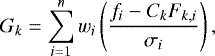
In orderto estimate the spectral type of HD 4113C, we used the SpeX Prism library of near-IR spectra of brown dwarfs (Burgasser 2014) using the splat python package (Burgasser et al. 2016). Each spectrum was flux calibrated to the distance of HD 4113. To compare the goodness of fit of each spectrum (Fk) to the observed combined IFS and IRDIS spectrum (f), we used the Gk statistic used by Cushing et al. (2008) and others, where each measurement is weighted by its spectral FWHM:
 (1)
(1)
with the weights given by 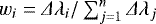 . Ck is a constant used to scale the flux of each spectrum, chosen to minimize Gk. We investigated the best fits with and without including the Ck factor to isolate the effects of the spectral shape and the absolute flux.
Each SpeX Prism spectrum was converted into the appropriate spectral resolution of each IFS measurement by convolution with a Gaussian. The FWHM used for the convolution was assumed to be 1.5× the separation between each wavelength channel. To predict the IRDIS fluxes, we used the transmission curves for the H2 and H3 filters.
Comparison with all objects with known distances in the SpeX Prism library shows that HD 4113C is most compatible with the coldest objects in the library, with spectral types of T8-T9 providing the best fit. When we excluded the Ck factor from scaling the flux of the SpeX Prism spectra, the individual flux values were marginally lower than any object in the library, leading to a stronger preference for late-T spectral types. This same trend is seen when considering the IFS and IRDIS results separately. In all cases, the only T9 object in the library gave the best fit to the spectrum, suggesting a most likely spectral type of T9.
The best fits to the observed spectrum are given by the objects UGPS J072227.51-054031.2 (Lucas et al. 2010, Gk = 2.86) and WISE J165311.05+444422.8 (Kirkpatrick et al. 2011, Gk = 3.22), field dwarfs of type T9 and T8, respectively. A comparison of the measured spectrum with those of these two objects is shown in Fig. 4.
Using the predicted H2 and H3 fluxes from the SpeX Prism Library, we produced the color-magnitude diagram in Fig. 5. The observed H2 flux is similar to the faintest objects in the library, adding additional weight to the idea that the companion is close to the T/Y transition. The 3 σ upper limit on the H2-H3 color is consistent with spectral types T7 and later.
To further constrain the physical properties of HD 4113C, we compared the observed spectral energy density to synthetic spectra for cool brown dwarfs from Morley et al. (2012), Morley et al. (2014) and Tremblin et al. (2015) using the same minimization technique as was used for the SpeX Prism Library. Each set of models gives fluxes as measured at the surface of the object and can be flux-scaled to the distance of HD 4113 after assuming a radius. We considered radii between 0.5–1.5 RJ when comparing the models.
The Morley et al. (2012) models include the effects of sulfide clouds at low temperatures and cover a range of effective temperatures Teff = 400–1300 K and surface gravities logg = 4–5.5, with condensate sedimentation efficiency coefficients fSED = 2–5. The Morley et al. (2014) models extend the previous models to lower temperatures by including water ice clouds and partly cloudy atmospheres. They cover a range of effective temperatures Teff = 200–450 K, surface gravities log g = 3–5, and condensate sedimentation efficiency coefficients fSED = 3–7, and assume that 50% of the surface is covered by clouds. The Tremblin et al. (2015) models include the effects of convection and non-equilibrium chemistry and cover a range of effective temperatures Teff = 200–1000 K and surface gravities logg = 4–5, with vertical mixing parameters logKzz = 6–8. The parameters of the best-fitting models are shown in Table 5.
For the Morley et al. (2012) models, lower temperature spectra fit the observed values more closely, with the best-fitting model being Teff = 600 K, log g = 5.0, fSED = 2, and R = 1.4 RJ. The model spectra are not strongly affected by changes in fSED in this regime of temperatureand logg, and for all fSED values in the grid, the same effective temperature and surface gravity provide the best fit. These models provide a reasonable fit to the data, but predict a higher H3 flux than our upper limits, and appear to underestimate the Y-band flux.
The Morley et al. (2014) models did not produce a good match to the observed data. The best-fitting model corresponds to Teff = 450 K, log g = 5, fSED = 5, and R = 1.5 RJ. These parameters are at the edge of the model grid, and the Gk value was significantly higher than the other model sets. They failed to simultaneously fit the fluxes of the J- and H-band peaks with a radius R < 1.5 RJ.
When comparing the data with the Tremblin et al. (2015) model spectra, we find best-fit parameters of Teff = 500 K, log g = 4.5, log Kzz = 6, and R = 1.5 RJ. Similar to the previous model set, these models have difficulty in reproducing the fluxes of the J and H peaks while constrained to R < 1.5 RJ.
The radius and temperature are highly correlated for each set of models (since Teff ∝ R−0.5 for a blackbody). Models with lower temperature provide a better fit to the shape of the
spectrum, but fail to reproduce the flux. When we fixed the radius to 1 RJ, the best-fit temperatures were 700 K for the Morley et al. (2012) grid and 600 K for the Tremblin et al. (2015) grid, with Gk values of 3.2and 5.1 respectively.
If the restriction on the radius is removed, the fits converge to temperatures of 300 K and 325 K for the Tremblin et al. (2015) and Morley et al. (2014) models with Gk values of 0.94 and 2.7, respectively, while the Morley et al. (2012) models prefer the lower edge of the model grid at 400 K with a Gk value of 1.6.These fits match the shape of the observed spectrum, but do not correspond to physically reasonable radii.
The best-fitting spectrum from the Morley et al. (2012) and Tremblin et al. (2015) model grids are shown in Fig. 4.
Becauseof the relatively low S/N of the spectrum, the lack of K and L photometry, and the use of only a single epoch of data, we caution that more work is needed before accurate limits can be placed on the effective temperature, radius, and surface gravity measurements.
The measured absolute photometry of HD 4113 C.
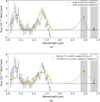 |
Fig. 4 Comparison of the observed spectrum of HD 4113C with similar ultracool dwarfs and brown dwarf atmosphere models. Top panel: measured spectrum of HD 4113C extracted from the IFS and IRDIS images. Two peaks are seen in the IFS spectrum at 1.07 μm and 1.27 μm, which correspond well with the spectral features seen in late-T dwarfs. The two best-fitting spectra from the SpeX Prism library are overplotted, and the flux is scaled to match HD 4113C. The predicted flux values for each datapoint are shown with filled circles, while the datapoints are marked with crosses. The FWHM of the IRDIS filters are shown with gray bars. Fitting was performed to the IFS and IRDIS data simultaneously. Bottom panel: same as top panel, this time showing the comparison between the observed spectrum and the best-fit spectra from the Morley et al. (2012) and Tremblin et al. (2015) models, using radii of 1.4 and 1.5 RJ, respectively. |
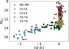 |
Fig. 5 Color-magnitude diagram showing the predicted H2-H3 colors and H2 absolute magnitudes for objects in the SpeX Prism Library. The flux of HD 4113C and the 3 σ upper limit on its H2-H3 color are shown with a red arrow. Its position is compatible with objects at the end of the T sequence, showing deep methane absorption indicative of T and Y dwarfs. |
Comparison of best-fitting model parameters extracted from the spectral fitting.
4.4 Orbit determination and dynamical masses
To constrain the orbital parameters of the planet and brown dwarf, we performed a combined fit to the RV and direct-imaging data. For this purpose, we used the 2016 IRDIS H2 astrometry and the astrometry extracted from the 2015 IFS YH combined image, both reported in Table 3.
The initial RV data analysis presented in this paper was accomplished using a set of online tools hosted by the Data & Analysis Center for Exoplanets (DACE)1, which performs a multiple Keplerian adjustment to the data as described in Delisle et al. (2016). It allowed us to derive initial conditions for a combined analysis of the direct-imaging and RV data, performed within a Bayesian formalism.
To model the observed data, a Keplerian was assigned to the inner planet (P = 526.57 d, m sini = 1.66MJup) that is only seen in the RV measurements. A second Keplerian was added to reproduce both the observed RV drift and the positions of the imaged brown dwarf companion.
The observed signal was modeled with two Keplerians and five RV offsets (one offset for each RV instrument). We modeled the noise using a nuisance parameter for each RV instrument (Gregory 2005). These nuisance parameters were added quadratically to the individual measurement errors. We combined the signal and the noise model into a likelihood function that was probed using emcee - a python implementation of the affine-invariant Markov chain Monte Carlo (MCMC) ensemble sampler (Foreman-Mackey et al. 2013; Goodman & Weare 2010). The full technical description of the combined data analysis is given in Appendix B, and we focus here on the data analysis results.
Despite possessing only two direct-imaging measurements and the partial RV coverage of the orbit, we were able to bring significant constraints on the geometry of the orbit and mass of HD 4113 C. The observed RV drift indeed displays a high peak-to-peak value of ~365 ms−1 over the 18 yr of CORALIE observations, setting a clear minimum mass boundary for the brown dwarf.
Within this framework and based on the MCMC posterior distribution, we are able to set confidence intervals for the orbital elements and physical parameters of HD 4113 C. At the 1 σ level, the period ranges between 87 yr and 134 yr, its semi-major axis is between 20.3 AU and 27.1 AU, and its mass is in the range 61–71 MJ. The eccentricity is well constrained with a value ranging between e = 0.31 and e = 0.46 at 1 σ.
The results of the MCMC analysis are summarized in Table 6, and the corresponding orbits are shown in Fig. 6. A mass-separation diagram based on the marginalized 2D posterior distribution is presented in Fig 7.
Orbital elements and companion properties derived from the posterior distribution of the two-Keplerian Model.
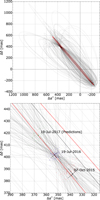 |
Fig. 6 Observed and predicted orbital motion of HD 4113 AC, shown as the relative projected position of HD 4113C. A series of orbits are plotted, drawn from the posterior distribution of the combined RV+imaging analysis. The bold red curve corresponds to the maximum likelihood solution. The bottom panel is a zoom of the orbit, centered on the date of the observations. |
4.5 Dynamics and formation
Table 6 shows that the eccentricity of HD 4113Ab is particularly high (eAb ≈ 0.9). The Lidov-Kozai mechanism (see Lidov 1962; Kozai 1962) has often been proposed to explain highly eccentric planetary orbits. In the case of HD 4113A b, this idea was raised at the time of its discovery by Tamuz et al. (2008). The observed RV was evidence of a high-mass, long-period companion that would naturally interact gravitationally with the planet.
Using the orbital parameters derived from the new RV and direct-imaging measurements, we are able to test the Lidov-Kozai scenario in more detail. We adopted the best-fitting (maximum likelihood) parameters for the planet and brown dwarf (see Table B.1) in order to have a coherent set of orbital elements. The only parameters that were unconstrained by the observations are the inclination (iAb) and the longitude of the ascending node (ΩAb) of the planet. We thus let these parameters vary. We also let the mass of the planet (MAb) vary according to its inclination, since the RV data constrain only its minimum mass (MAb siniAb). We ran a set of 1681 (41 × 41) simulations of the system using the GENGA integrator (see Grimm & Stadel 2014), with iAb varying in the range [5°, 175°] (MAb ∈ [1.67 − 19.21]), and ΔΩ= ΩAb − ΩC varying in the range [−180°, 180°]. The time step was set to 0.001 yr and the orbits were integrated for 1 Myr, including the effects of General Relativity.
Figure 8 shows the initial mutual inclination between the orbits of the planet and brown dwarf (iAb-C), plotted as afunction of the two unknown parameters. Figure 9 shows the minimum value reached by the planet eccentricity during the whole simulation. Unstable integrations were stopped and are drawn in white in Fig. 9. In particular, the simulations in which the planet approaches the star by less than 0.005 AU (close to one stellar radius) were stopped. Depending on the initial parameters (iAb, ΩAb), strong Lidov-Kozai cycles are observed, and the eccentricity of the planet could reach very low values (blue points in Fig. 9). Figure 10 shows an example of a simulation where strong Lidov-Kozai cycles are observed. It is therefore possible that the planet formed on a quasi-circular orbit and that the observed eccentricity (0.9) is the result of Lidov-Kozaioscillations with the observed brown dwarf.
From Fig. 9 we were able to derive constraints on the missing orbital elements of the planet (iAb, ΩAb) for the system to be stable (i.e., not located in a white region), and for the planet to have formed with a low eccentricity (blue parts). We note that several effects might modify the results shown in Fig. 9. Considerable uncertainties remain on several of the orbital parameters for the brown dwarf, and changes in these orbital parameters would be reflected in Fig. 9. Moreover, in some of the simulations shown here, the eccentricity of the planet reaches very high values. In this case, the time step we used (0.001 yr) is not sufficiently small to correctly model the periastron passage, and some orbits that are detected as unstable (white parts in Fig. 9) might be stable (and vice versa). In addition, in the very high eccentricity cases, tides may play an important role. The combination of the Lidov-Kozai mechanism and tides can even induce an inward migration of the planet (see Wu & Murray 2003; Fabrycky & Tremaine 2007; Correia et al. 2011). In this scenario, the planet initially forms at a larger distance to the star and with a quasi-circular orbit. It then undergoes strong Lidov-Kozai oscillations, which brings the planet very close to the star at periastron. In addition to shrinking the planet orbit (decreasing semi-major axis), tides (and general relativity) tend to damp the amplitude of the Kozai oscillations. The maximum eccentricity reached during a Lidov-Kozai cycle does not change much, but the minimum eccentricity increases. When the Lidov-Kozai amplitude vanishes, the eccentricity is simply damped from a very high value down to zero. If HD 4113A b follows this path, the amplitude of the Lidov-Kozaicycles could have been already significantly damped. Therefore, the minimum eccentricity reached by the planet during a Lidov-Kozai cycle might be high, even if the planet initially formed on a quasi-circular orbit.
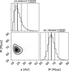 |
Fig. 7 Marginalized 1D and 2D posterior distributions of the mass vs. semi-major axis corresponding to the global fit of the RV and direct-imaging models. Confidence intervals at 2.275%, 15.85%, 50.0%, 84.15%, and 97.725% are overplotted on the 1D posterior distributions, while the median ± 1 σ values are given at the top of each 1D distribution. 1, 2, and 3 σ contour levels are overplotted on the 2D posterior distribution. |
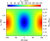 |
Fig. 8 Initial mutual inclination between the planet and brown dwarf orbits (iAb-C) as a functionof the planet inclination (iAb) and longitude of the ascending node (ΔΩ = ΩAb − ΩC). |
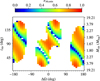 |
Fig. 9 Minimum value reached by the planet eccentricity during the 1 Myr of integration (eAb,min), as a functionof the initial inclination of the planet (iAb), and longitude of the ascending node (ΔΩ = ΩAb − ΩC). White points correspond to unstable simulations that stopped before 1 Myr. |
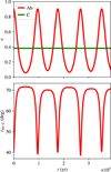 |
Fig. 10 Example of temporal evolution of the eccentricities of the planet and the brown dwarf (top) and their mutual inclination (bottom). The initial conditions are set using the best-fitting parameters (see Table B.1), and iAb = 128.25° (MAb ≈ 2.13 MJ), and ΔΩ = 18°. This corresponds to an initial mutual inclination of about 40.47°. The minimum value of the planet eccentricity is about 0.06 and is reached when the mutual inclination reaches about 72°. |
5 Discussion and conclusion
The HD 4113 system is an important laboratory for studying a range of issues in stellar and substellar physics. The primary star, HD 4113A, hosts a planetary companion on a highly eccentric orbit. By fitting to 28 years of RV data, we updated the orbital parameters from those presented at the time of its discovery by Tamuz et al. (2008). In addition, we presented high-contrast imaging data that revealed the nature of a long-period RV signal as originating from a cool brown dwarf companion.
The imaging data show that the brown dwarf has a contrast in the SPHERE H2 filter of 13.35 mag and a deep methane absorption feature that causes it to have a H2-H3 color of > 1.45 mag. Using the COND isochrones, the H2 and synthetic J-band absolute fluxes are consistent with masses of 36 ± 5 MJ and 29 ± 5 MJ, respectively.
Fitting to the observed spectrum from IFS and IRDIS allowed us to estimate the effective temperature, spectral type, radius, and surface gravity of HD 4113C. Through comparison with the SpeX Prism Library of brown dwarf spectra, we found that it is most consistent with the coldest objects in the library, with the best match coming from a T9 field dwarf. Additional support for a late-T spectral type comes from the position of HD 4113C on the H2-H3 color-magnitude diagram (Fig. 5).
Using the atmosphere models of Morley et al. (2012) and Tremblin et al. (2015), we found best-fit values of Teff = 500–600 K, log g = 4.5–5, and R = 1.4–1.5 RJ.
However, because we relied on a single-epoch spectrum with moderate S/N, additional data with high S/N covering a wider range of wavelengths are needed to further characterize HD 4113C and to confirm the spectral type, effective temperature, radius, and surface gravity estimates. The radius estimate is much higher than predicted for old, high-mass brown dwarfs, suggesting that more work may be needed to understand the system parameters. In particular, additional spectra to constrain the shape of the J- and H-band peaks and photometric measurements at longer wavelengths (K and L band) would help in this task.
We placed constraints on the orbital and physical parameters of HD 4113C through orbital fitting to the RV and imaging data. This suggests a mass of  MJ, and a moderate eccentricity of
  . With longer time baselines for both the imaging and RV data, orbital fitting will provide tighter constraints on the mass, and this system could act as a useful mass-luminosity benchmark for late-T dwarfs.
When comparing the derived properties of HD 4113C to those of other directly imaged companions to main-sequence stars, we found a strong correspondence with GJ 504b (Kuzuhara et al. 2013) in many aspects. The late-T spectral type and J-band absolute magnitude (~18.7 mag) in particular suggest that GJ 504b is a useful analog. Both objects also orbit metal-enriched, solar-like stars, with recent data suggesting that GJ 504 may also have a solar-like age of ~4 Gyr (Fuhrmann & Chini 2015).
In addition to GJ 504b, HD 4113C joins a growing list of cool, T dwarf companions imaged around main-sequence stars, including the T4.5-T6 planet 51 Eri b (Macintosh et al. 2015) and the T8 brown dwarf GJ 758 B (Thalmann et al. 2009).
HD 4113C also joins HD 19467B (Crepp et al. 2014) as the second imaged T dwarf with a measured RV acceleration that allows it to be used as a benchmark object. While HD 19467B appears to have a higher effective temperature of ~1000 K, its dynamical mass and age are similar to that of HD 4113C.
Through dynamical simulations, we showed that the observed high eccentricity (e ~ 0.9) of the giant planet HD 4113A b could be the result of strong Lidov-Kozai cycles caused by interactions with the orbit of the imaged brown dwarf. For certain ranges of the unknown orbital parameters iAb and ΔΩ, eccentricity oscillations of >0.8 are observed, typically with an oscillation period of 104 −105 yr. This raises the possibility that HD 4113A b formed on an initially quasi-circular orbit and subsequently underwent eccentricity excitation through interaction with HD 4113C.
However, further questions about the formation of HD 4113A b remain. The brown dwarf companion would be expected to truncate the circumstellar disk of HD 4113A at 1/2 - 1/3 of its semi-major axis (Artymowicz & Lubow 1994), which corresponds to 7–11 AU on its present orbit. Forming a planetary companion in such an active dynamical system within a truncated disk may prove challenging.
An exciting prospect for further characterization of this system are the future Gaia data releases. The astrometric signal of the giant planet HD 4113A b should be detectable with Gaia and will give an accurate inclination measurement. The planet will introduce astrometric motion with a peak-to-peak amplitude of at least 0.08 mas. In addition, a long-term drift corresponding to the HD 4113A-C orbit should also be visible. With a 10 yr dataset, this would introduce a 13 mas drift in the position of HD 4113A, with a maximum deviation of 0.8 mas from linearity. Even with the current 3 yr time baseline, the curvature induced by HD 4113C should have an amplitude of ~ 0.1 mas.
The combination of Gaia astrometry with future RV and imaging datasets will allow for much tighter constraints on the orbits and physical parameters of each component. Most critically, Gaia astrometry will give a first measurement of the unknown orbital parameters of the planet. This will be crucial for studying the Lidov-Kozai interactions and stability of the system, by significantly reducing the parameter range to explore and by resolving the degeneracy with the unknown planet mass. Moreover, the combination of more accurate mass measurements of the brown dwarf with improved spectroscopy and photometry will be useful for comparison with atmosphere and evolution models.
While the imaging data do confirm the existence of a wide brown dwarf-mass companion seen in the RVs, the observed MCMC posterior for the mass of HD 4113C shows an apparent underlying inconsistency between the input data. As seen in Fig. 7, the predicted mass is close to the stellar/substellar boundary, while the spectrum obtained through direct imaging shows an extremely cool temperature that would suggest a much lower mass.
This combination of the dynamical mass, age, and low temperature of the companion presents a challenge to brown dwarf cooling models. The COND models predict that a 66 MJ object would have cooled to 1200 ± 170K at  Gyr, significantly higher than the 500–600 K estimates from the best-fit spectral models.
However, there are several scenarios that may explain this apparent disagreement. Most notably, the newly detected companion may be an unresolved brown dwarf binary system, leading to an increased dynamical mass and radius estimate without greatly influencing the shape of the observed spectrum. In the case of an equal-mass binary, this would relax the tension between the temperature and radius in the spectral model fits, allowing for a pair of 500–600 K objects with radii of 1 RJ to provide a good match to the observed data. This is close to the prediction of 640 ± 80 K from the COND models, based on a 33 MJ object at  Gyr. In this case, given the lack of extended structure visible in the companion PSF, we can only place an upper limit of 2 AU on the current projected separation of such a system. More stringent constraints may be given by considering the stability of the system as a whole.
An alternative possibility is that the presence of an additional companion to HD 4113A could have biased the RV data and caused an overestimate of the dynamical mass. For example, the long-term curvature in the RVs may be caused by an unseen planetary or brown dwarf companion at a smaller separation, while the imaged companion may be a longer-period intermediate-mass brown dwarf that contributes only a linear drift to the observed radial velocities.
We investigated this possibility numerically in our orbit fitting through the addition of a third body (“HD 4113D”) at intermediate periods (25 [yr] < P <100 [yr]), which is notdetected by SPHERE and which absorbs most of the RV drift.
Repeating the MCMC analysis resulted in a wide range of solutions because of the modest constraints of the observations with respect to the complexity of the model. However, we were able to extract from the posterior distribution a sub-sample of good solutions with a significantly lower mass for the brown dwarf imaged by SPHERE. In Table 7 we show one example with a dynamical mass of 40 MJ for the imaged companion, similar to the isochronal mass estimates from the SPHERE data.
While the present data do not provide any way to distinguish between this scenario and the two-Keplerian model, additional imaging, RV, and astrometric data will allow this idea to be investigated further. With several imaging datasets taken over a much longertime period, the orbit calculated from the imaging data alone could be compared to that expected from the RV data. Any inconsistencies in the estimated parameters would then indicate that an additional body may be present in the system.
However, the three-Keplerian scenario fails to explain the higher-than-expected flux (or equivalently, radius) of the imaged companion given its estimated effective temperature. Of these hypotheses, the binary brown dwarf scenario presents a more compelling case because of its capacity to explain all of the properties that have been explored in this paper, and because the stability of the system as a whole is clearer. Despite this, given the current data and the orbital coverage, more work is needed to firmly establish the underlying cause of the mass discrepancy.
Example of consistent orbital elements and companion properties for a three-Keplerian model compatible with our observations.
Acknowledgements
This work has been carried out within the frame of the National Centre for Competence in Research “PlanetS” supported by the Swiss National Science Foundation (SNSF). This publication makes use of The Data & Analysis Center for Exoplanets (DACE), which is a facility based at the University of Geneva (CH) dedicated to extrasolar planet data visualisation, exchange, and analysis. DACE is a platform of the Swiss National Centre of Competence in Research (NCCR) PlanetS, federating the Swiss expertise in Exoplanet research. The DACE platform is available at https://dace.unige.ch. SPHERE is an instrument designednd built by a consortium consisting of IPAG (Grenoble, France), MPIA (Heidelberg, Germany), LAM (Marseille, France), LESIA (Paris, France), Laboratoire Lagrange (Nice, France), INAF - Osservatorio di Padova (Italy), Observatoire Astronomique de l’Université de Genève (Switzerland), ETH Zurich (Switzerland), NOVA (Netherlands), ONERA (France) and ASTRON (Netherlands) in collaboration with ESO. SPHERE was funded by ESO, with additional contributions from CNRS (France), MPIA (Germany), INAF (Italy), FINES (Switzerland) and NOVA (Netherlands). SPHERE also received funding from the European Commission Sixth and Seventh Framework Programmes as part of the Optical Infrared Coordination Network for Astronomy (OPTICON) under grant number RII3-Ct-2004-001566 for FP6 (2004-2008), grant number 226604 for FP7 (2009-2012) and grant number 312430 for FP7 (2013-2016). We acknowledge financial support from the Programme National de Planétologie (PNP) and the Programme National de Physique Stellaire (PNPS) of CNRS-INSU. This work has also been supported by a grant from the French Labex OSUG@2020 (Investissements d’avenir - ANR10 LABX56). This work has made use of data from the European Space Agency (ESA) mission Gaia (http://www.cosmos.esa.int/gaia), processed by the Gaia Data Processing and Analysis Consortium (DPAC, http://www.cosmos.esa.int/web/gaia/dpac/consortium). Funding for the DPAC has been provided by national institutions, in particular the institutions participating in the Gaia Multilateral Agreement. This publication makes use of data products from the Two Micron All Sky Survey, which is a joint project of the University of Massachusetts and the Infrared Processing and Analysis Center/California Institute of Technology, funded by the National Aeronautics and Space Administration and the National Science Foundation. J.H. is supported by the Swiss National Science Foundation (SNSF), and the French National Research agency through the GIPSE grant ANR-14-CE33-0018. This research has benefitted from the SpeX Prism Spectral Libraries, maintained by Adam Burgasser at http://pono.ucsd.edu/~adam/browndwarfs/spexprism.
Appendix A: NACO L-band direct-imaging data
We present here the results of the 2013-08-21 data taken with NACO (Program 091.C-0721, PI Ségransan). The observing sequence consisted of 419 cubes of 128 frames, each with an exposure time of 0.2 s. The maximum field rotation during the sequence was 112 deg. This dataset was processed with the GRAPHIC pipeline (Hagelberg et al. 2016), using a similar reduction sequence as for the SPHERE data described in Sect. 3, without the application of SDI. Before PCA was applied, the data were binned into 419 frames by taking the median over each cube.
The detection limits and final reduced image are presented in Fig. A.1. The companion was not detected in these data, with the 5 σ contrast limit at the location of the SPHERE detection being 10.3 mag. At its predicted location based on the orbital fit in Sec. 4.4, the 5 σ contrast limit is 10.0 mag. From the BHAC15 and COND isochrones, these correspond to mass limits of 73 MJ.
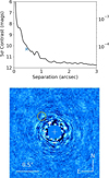 |
Fig. A.1 5 σ contrast obtained from the NACO L’ data taken in 2013. The separation and predicted contrast from the orbit fitting is marked with a blue cross. At this separation, the corresponding limit is 10.3 mag. Despite the close correspondence between the predicted contrast and the 5 σ limits, we do not unambiguously detect the companion. The final reduced image is also shown, after removing 150 PCA modes. Thepredicted position for the 2013 epoch is shown with a yellow circle. While the contrast curve has been corrected for companion self-subtraction introduced by the PCA procedure, the image has not. Through injection of fake companions, we estimate a 35% flux loss for objects at the predicted separation of HD 4113 C. |
From the COND models, the expected L-band contrast is 10.3 mag using the dynamical mass of 66 MJ. The H2 and J-band contrasts predict L-band contrasts of 13.9 and 14.9 mag, respectively.
Appendix B: MCMC details
B.1 Likelihood function
Throughoutthis section, we assume that the observed signals are modeled with two independent Keplerians and five RV offsets corresponding to the number of RV instruments. The noise associated with each measurement is assumed to be independently drawn from a normal distribution with zero mean N(0, σi). The observed signal yi is written in Eq. (B.1) as a sum between the model fi(X) for parameters X and a realization of the noise ei. yi represents both the measured radial velocities and the direct-imaging data (i.e., ρ, PA)
 (B.1)
(B.1)
The likelihood function is given in Eq. (B.2), where σi is the estimated error on each data point yi and σ0 is an additional white-noise parameter (see Gregory 2005) added to each RV instrument. These nuisance parameters account for any additional noise sources that were not included in the error bars of the measurements,
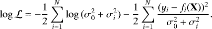 (B.2)
(B.2)
B.2 Choice of parameters
Our model for the RV measurements is composed of five linear terms: the systematic RV of HIRES (γHIRES), the offset between CORAVEL and HIRES (ΔV (CORA − HIRES)), the offset between CORALIE-98 and HIRES (ΔV (C98 − HIRES)), the offset between CORALIE-07 and HIRES (ΔV (C98 − HIRES)), and the offset between CORALIE-14 and HIRES (ΔV (C14 − HIRES)). The CORALIE offsets originate from the different instrument upgrades performed over the 19 years of observations.
We modeled the Keplerian corresponding to HD 4113A b with the parameters log P, log K, e, ω, and M0, using the period P, the RV semi-amplitude K, eccentricity e, the argument of periastron ω, and the mean anomaly M0 at a given reference epoch (tref = 2 455 500.0 d).
We used a different set of variables to model HD 4113C to reduce correlations between them. We used log P,  ,
,  , mC sini, TMIN(rv), i, and Ω. The last four variables correspond to the minimum mass of the brown dwarf, the date at which the minimum RV occurs, the orbital inclination, and the longitude of the ascending node.
B.3 Choice of priors
All adjusted parameters have uniform priors, with the exception of the RV offsets. We applied priors to the RV offsets between the CORALIE instruments, ΔV (C98 − C07) = N(0, 5) and ΔV (C98 − C07) = N(12, 5) has been calibrated using RV standard stars that were observed with both C98 and C07, allowing us to adopt a Gaussian prior centered on zero with a standard deviation of 5 ms−1. The prior on the offset between CORAVEL and CORALIE is a truncated normal distribution defined as ΔV (CORA − C07) = TN(−51, 200, −200, 200).
We alsoincluded a set of priors for the parallax and masses of the system HD 4113AC based on our external knowledge. We adopted a Gaussian prior for the parallax based on the latest Gaia measurements, and we chose a uniform prior for the mass of HD 4113C with an upper at half of the mass of the primary star. For the mass of HD 4113 A, we used a split normal distribution with asymmetric standard deviation taken from Table 1.
B.4 MCMC runs
We probed the model parameter space using emcee, a python implementation of the affine-invariant Markov chain Monte Carlo (MCMC) ensemble sampler (Foreman-Mackey et al. 2013; Goodman & Weare 2010) and the likelihood function described in the above subsections.
We ran several MCMC simulations. For the first MCMC run, we performed 4 500 iterations using 50 walkers with initial conditions drawn from the solution obtained using DACE. A first set of parameter posterior distributions were derived using a burn-in phase of 1 500 iterations. In order to obtain a statistically robust sample, we ran a second MCMC simulation with 100 walkers drawn from the posterior of our first simulation with a total of 800 000 iterations, which guarantees a faster convergence to equilibrium.
We derive our final sample by
-
discarding 5% of the walkers based on the properties of each walker posterior distribution (standard deviation, maximum value, median value);
-
computing the correlation timescale (τ) of each walker and discarding those with τ > 500;
-
eliminating the initialization bias by discarding the first 20τ elementsof each walker (following Sokal 1997); and
-
sampling each walker according to their coherence time to build the final statistical sample.
This returned a sample of 61 200 independentdata points that allowed us to retrieve and characterize the underlying parameter distributions with a  accuracy (Sokal 1997), which is close to the 3 σ confidence intervals.
Figures B.1 and B.2 show the marginalized 1D and 2D posterior distributions of the Keplerian model parameters of the giant planet HD 4113 A b. As illustrated, the distributions are close to Gaussian, with small linear correlations. The corresponding parameters and confidence intervals are listed in Table B.1.
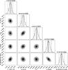 |
Fig. B.1 Marginalized 1D and 2D posterior distributions of the model parameters corresponding to the global fit of the RV and direct-imaging models for HD 4113 A b. Confidence intervals at 2.275%, 15.85%, 50.0%, 84.15%, and 97.725% are overplotted on the 1D posterior distribution, while the median ± 1 σ values are given at the top of each 1D posterior distributions. 1, 2, and 3 σ contour levels are overplotted on the 2D posterior distributions. The model parameters adjusted during the MCMC run are shown (P, K, e, ω, and M0). |
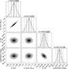 |
Fig. B.2 Same as Fig. B.1, showing the additional parameters derived from the MCMC posterior samples (a, m sin i, Tp, and λ0) for HD 4113A b. |
Priors and parameters probed with the MCMC.
The case of HD 4113 C is less straightforward because of strong correlations in the 2D posterior distributions (see Fig. B.3 and B.4). Furthermore, most of the 1D distributions are non-Gaussian, which makes the use of mean value and error bars potentially misleading. We instead prefer to list the values corresponding to the maximum likelihood, the sample median, and the mode of the distribution in Table B.1. Confidence intervals corresponding to 1 σ and 2 σ are also given for each parameter, as well as the prior distribution we used.
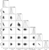 |
Fig. B.3 Same as Fig. B.1 for HD 4113C, showing the correlations and marginalized posterior distributions for the model parameters adjusted during the MCMC run (P,
K,
|


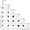 |
Fig. B.4 Same as Fig. B.2, showing the additional parameters derived from the MCMC posterior samples for HD 4113C (a, m, e, ω, Tp, and λ0). |
References
- Allard, F., Homeier, D., & Freytag, B. 2012, Phil. Trans. R. Soc. London, Ser. A, 370, 2765 [Google Scholar]
- Artymowicz, P., & Lubow, S. H. 1994, ApJ, 421, 651 [NASA ADS] [CrossRef] [Google Scholar]
- Baraffe, I., Chabrier, G., Barman, T. S., Allard, F., & Hauschildt, P. H. 2003, A&A, 402, 701 [NASA ADS] [CrossRef] [EDP Sciences] [Google Scholar]
- Baraffe, I., Homeier, D., Allard, F., & Chabrier, G. 2015, A&A, 577, A42 [NASA ADS] [CrossRef] [EDP Sciences] [Google Scholar]
- Beuzit, J.-L., Feldt, M., Dohlen, K., et al. 2008, in Proc. SPIE, 7014 [Google Scholar]
- Bohlin, R. C. 2007, in The Future of Photometric, Spectrophotometric and Polarimetric Standardization, ed. C. Sterken, ASP Conf. Ser., 364, 315 [NASA ADS] [Google Scholar]
- Burgasser, A. J. 2014, in Astron. Soc. India Conf. Ser., 11 [Google Scholar]
- Burgasser, A. J., Aganze, C., Escala, I., et al. 2016, in Am. Astron. Soc. Meeting Abstracts, 227, 434.08 [NASA ADS] [Google Scholar]
- Butler, R. P., Vogt, S. S., Laughlin, G., et al. 2017, AJ, 153, 208 [NASA ADS] [CrossRef] [Google Scholar]
- Correia, A. C. M., Laskar, J., Farago, F., & Boué, G. 2011, Celestial Mech. Dyn. Astron., 111, 105 [Google Scholar]
- Crepp, J. R., Johnson, J. A., Howard, A. W., et al. 2014, ApJ, 781, 29 [NASA ADS] [CrossRef] [Google Scholar]
- Cushing, M. C., Marley, M. S., Saumon, D., et al. 2008, ApJ, 678, 1372 [NASA ADS] [CrossRef] [Google Scholar]
- Delfosse, X., Forveille, T., Ségransan, D., et al. 2000, A&A, 364, 217 [NASA ADS] [Google Scholar]
- Delisle, J.-B., Ségransan, D., Buchschacher, N., & Alesina, F. 2016, A&A, 590, A134 [NASA ADS] [CrossRef] [EDP Sciences] [Google Scholar]
- Dohlen, K., Langlois, M., Saisse, M., et al. 2008, in Ground-based and Airborne Instrumentation for Astronomy II, Proc. SPIE, 7014, 70143L [CrossRef] [Google Scholar]
- Fabrycky, D., & Tremaine, S. 2007, ApJ, 669, 1298 [NASA ADS] [CrossRef] [Google Scholar]
- Foreman-Mackey, D., Hogg, D. W., Lang, D., & Goodman, J. 2013, PASP, 125, 306 [CrossRef] [Google Scholar]
- Fuhrmann, K., & Chini, R. 2015, ApJ, 806, 163 [NASA ADS] [CrossRef] [Google Scholar]
- Gaia Collaboration, (Brown, A. G. A., et al.) 2016, A&A, 595, A2 [NASA ADS] [CrossRef] [EDP Sciences] [Google Scholar]
- Goodman, J., & Weare, J. 2010, Comm. App. Math. Comp. Sci., 5, 65 [Google Scholar]
- Gregory, P. C. 2005, Bayesian Logical Data Analysis for the Physical Sciences: A Comparative Approach with ‘Mathematica’ Support (Cambridge University Press) [Google Scholar]
- Grimm, S. L., & Stadel, J. G. 2014, ApJ, 796, 23 [NASA ADS] [CrossRef] [Google Scholar]
- Hagelberg, J. 2014, Theses, Université Genève, Switzerland [Google Scholar]
- Hagelberg, J., Ségransan, D., Udry, S., & Wildi, F. 2016, MNRAS, 455, 2178 [NASA ADS] [CrossRef] [Google Scholar]
- Kirkpatrick, J. D., Cushing, M. C., Gelino, C. R., et al. 2011, ApJS, 197, 19 [NASA ADS] [CrossRef] [Google Scholar]
- Kozai, Y. 1962, AJ, 67, 591 [Google Scholar]
- Kuzuhara, M., Tamura, M., Kudo, T., et al. 2013, ApJ, 774, 11 [NASA ADS] [CrossRef] [Google Scholar]
- Lidov, M. L. 1962, Planet. Space Sci., 9, 719 [NASA ADS] [CrossRef] [Google Scholar]
- Lovis, C., Dumusque, X., Santos, N. C., et al. 2011, ArXiv e-prints [arXiv:1107.5325] [Google Scholar]
- Lucas, P. W., Tinney, C. G., Burningham, B., et al. 2010, MNRAS, 408, L56 [NASA ADS] [CrossRef] [Google Scholar]
- Macintosh, B. A., Graham, J. R., Palmer, D. W., et al. 2008, Proc. SPIE, 7015 [Google Scholar]
- Macintosh, B., Graham, J. R., Barman, T., et al. 2015, Science, 350, 64 [NASA ADS] [CrossRef] [Google Scholar]
- Maire, A.-L., Langlois, M., Dohlen, K., et al. 2016, Proc. SPIE, 9908, 34 [Google Scholar]
- Marmier, M. 2014, PhD thesis, Geneva Observatory, University of Geneva, Switzerland [Google Scholar]
- Mawet, D., Milli, J., Wahhaj, Z., et al. 2014, ApJ, 792, 97 [NASA ADS] [CrossRef] [Google Scholar]
- Mesa, D., Gratton, R., Zurlo, A., et al. 2015, A&A, 576, A121 [NASA ADS] [CrossRef] [EDP Sciences] [Google Scholar]
- Montagnier, G. 2008, Theses, Université Joseph-Fourier - Grenoble I, France [Google Scholar]
- Morley, C. V., Fortney, J. J., Marley, M. S., et al. 2012, ApJ, 756, 172 [NASA ADS] [CrossRef] [Google Scholar]
- Morley, C. V., Marley, M. S., Fortney, J. J., et al. 2014, ApJ, 787, 78 [NASA ADS] [CrossRef] [Google Scholar]
- Moutou, C., Vigan, A., Mesa, D., et al. 2017, A&A 602, A87 [NASA ADS] [CrossRef] [EDP Sciences] [Google Scholar]
- Mowlavi, N., Eggenberger, P., Meynet, G., et al. 2012, A&A, 541, A41 [NASA ADS] [CrossRef] [EDP Sciences] [Google Scholar]
- Mugrauer, M., Ginski, C., & Seeliger, M. 2014, MNRAS, 439, 1063 [NASA ADS] [CrossRef] [Google Scholar]
- Pavlov, A., Möller-Nilsson, O., Feldt, M., et al. 2008, in Advanced Software and Control for Astronomy II, Proc. SPIE, 7019, 701939 [CrossRef] [Google Scholar]
- Rajpurohit, A. S., Reylé, C., Allard, F., et al. 2013, A&A, 556, A15 [NASA ADS] [CrossRef] [EDP Sciences] [Google Scholar]
- Santos, N. C., Mayor, M., Naef, D., et al. 2002, A&A, 392, 215 [NASA ADS] [CrossRef] [EDP Sciences] [Google Scholar]
- Ségransan, D., Udry, S., Mayor, M., et al. 2010, A&A, 511, A45 [NASA ADS] [CrossRef] [EDP Sciences] [Google Scholar]
- Skrutskie, M. F., Cutri, R. M., Stiening, R., et al. 2006, AJ, 131, 1163 [NASA ADS] [CrossRef] [Google Scholar]
- Smith, W. H. 1987, PASP, 99, 1344 [NASA ADS] [CrossRef] [Google Scholar]
- Sokal, A. 1997, in Functional integration: basics and applications, Proceedings of a NATO Advanced Study Institute, Cargèse, France, September 1–14, 1996 (New York, NY: Plenum Press), 131 [Google Scholar]
- Soummer, R., Aime, C., & Falloon, P. E. 2003, A&A, 397, 1161 [NASA ADS] [CrossRef] [EDP Sciences] [Google Scholar]
- Soummer, R., Pueyo, L., & Larkin, J. 2012, ApJ, 755, L28 [NASA ADS] [CrossRef] [Google Scholar]
- Tamuz, O., Ségransan, D., Udry, S., et al. 2008, A&A, 480, L33 [NASA ADS] [CrossRef] [EDP Sciences] [Google Scholar]
- Thalmann, C., Carson, J., Janson, M., et al. 2009, ApJ, 707, L123 [NASA ADS] [CrossRef] [Google Scholar]
- Tremblin, P., Amundsen, D. S., Mourier, P., et al. 2015, ApJ, 804, L17 [NASA ADS] [CrossRef] [Google Scholar]
- Udry, S., Mayor, M., Naef, D., et al. 2000, A&A, 356, 590 [NASA ADS] [Google Scholar]
- Vigan, A., Moutou, C., Langlois, M., et al. 2010, MNRAS, 407, 71 [NASA ADS] [CrossRef] [Google Scholar]
- Wu, Y., & Murray, N. 2003, ApJ, 589, 605 [NASA ADS] [CrossRef] [EDP Sciences] [Google Scholar]
The DACE platform is available at http://dace.unige.ch while the online tools to analyze RV data can be found in the section Observations =>Radial Velocities.
All Tables
Orbital elements and companion properties derived from the posterior distribution of the two-Keplerian Model.
Example of consistent orbital elements and companion properties for a three-Keplerian model compatible with our observations.
All Figures
|
Fig. 1 Radial velocity measurements of HD 4113A taken with CORALIE (blue dots for data taken before the 2007 upgrade, and purple dots for data taken later) and with HIRES (orange dots), covering the time period from October 1999 to September 2017. Four CORAVEL measurements from as early as May 1989 are also included (black dots), extending the time baseline to 28 years. The top panel represents the observed CORALIE RV time series with the eccentric-orbit model of thegiant planet HD 4113A b as well as the long-term drift corresponding to HD 4113 C. The middle panel shows a phase-folded representation of the RV orbit of HD 4113A b, while the bottom panel shows the predicted and observed RVs for the orbit of HD 4113C after subtracting the signal produced by HD 4113A b. Several possible orbits drawn from the output of our MCMC procedure are shown. The bold red curve represents the maximum likelihood solution. |
| In the text | |
|
Fig. 2 PSF-subtracted images from each dataset and epoch. For the 2016 dataset, the IRDIS H2, H3, and SDI (H2-H3) reductions are shown, while we show only the 2015 IRDIS SDI (K1-K2) reduction. We also show a weighted combination of the IFS SDI images for each epoch. Each IFS wavelength channel was weighted by the average flux predicted by the best-fitting Morley et al. (2012) and Tremblin et al. (2015) models. The strong detection of the companion in H2 and the lack of a H3 counterpart indicates the presence of strong methane absorption. All images have the same scale and orientation, and were generated by removing 20 PCA modes. |
| In the text | |
|
Fig. 3 5 σ contrast obtained for the four IRDIS datasets (K1 and K2 from the 2015 data, and H2 and H3 from the 2016 data). The measured separation and contrast of the companion detected in the H2 band is marked in red. |
| In the text | |
|
Fig. 4 Comparison of the observed spectrum of HD 4113C with similar ultracool dwarfs and brown dwarf atmosphere models. Top panel: measured spectrum of HD 4113C extracted from the IFS and IRDIS images. Two peaks are seen in the IFS spectrum at 1.07 μm and 1.27 μm, which correspond well with the spectral features seen in late-T dwarfs. The two best-fitting spectra from the SpeX Prism library are overplotted, and the flux is scaled to match HD 4113C. The predicted flux values for each datapoint are shown with filled circles, while the datapoints are marked with crosses. The FWHM of the IRDIS filters are shown with gray bars. Fitting was performed to the IFS and IRDIS data simultaneously. Bottom panel: same as top panel, this time showing the comparison between the observed spectrum and the best-fit spectra from the Morley et al. (2012) and Tremblin et al. (2015) models, using radii of 1.4 and 1.5 RJ, respectively. |
| In the text | |
|
Fig. 5 Color-magnitude diagram showing the predicted H2-H3 colors and H2 absolute magnitudes for objects in the SpeX Prism Library. The flux of HD 4113C and the 3 σ upper limit on its H2-H3 color are shown with a red arrow. Its position is compatible with objects at the end of the T sequence, showing deep methane absorption indicative of T and Y dwarfs. |
| In the text | |
|
Fig. 6 Observed and predicted orbital motion of HD 4113 AC, shown as the relative projected position of HD 4113C. A series of orbits are plotted, drawn from the posterior distribution of the combined RV+imaging analysis. The bold red curve corresponds to the maximum likelihood solution. The bottom panel is a zoom of the orbit, centered on the date of the observations. |
| In the text | |
|
Fig. 7 Marginalized 1D and 2D posterior distributions of the mass vs. semi-major axis corresponding to the global fit of the RV and direct-imaging models. Confidence intervals at 2.275%, 15.85%, 50.0%, 84.15%, and 97.725% are overplotted on the 1D posterior distributions, while the median ± 1 σ values are given at the top of each 1D distribution. 1, 2, and 3 σ contour levels are overplotted on the 2D posterior distribution. |
| In the text | |
|
Fig. 8 Initial mutual inclination between the planet and brown dwarf orbits (iAb-C) as a functionof the planet inclination (iAb) and longitude of the ascending node (ΔΩ = ΩAb − ΩC). |
| In the text | |
|
Fig. 9 Minimum value reached by the planet eccentricity during the 1 Myr of integration (eAb,min), as a functionof the initial inclination of the planet (iAb), and longitude of the ascending node (ΔΩ = ΩAb − ΩC). White points correspond to unstable simulations that stopped before 1 Myr. |
| In the text | |
|
Fig. 10 Example of temporal evolution of the eccentricities of the planet and the brown dwarf (top) and their mutual inclination (bottom). The initial conditions are set using the best-fitting parameters (see Table B.1), and iAb = 128.25° (MAb ≈ 2.13 MJ), and ΔΩ = 18°. This corresponds to an initial mutual inclination of about 40.47°. The minimum value of the planet eccentricity is about 0.06 and is reached when the mutual inclination reaches about 72°. |
| In the text | |
|
Fig. A.1 5 σ contrast obtained from the NACO L’ data taken in 2013. The separation and predicted contrast from the orbit fitting is marked with a blue cross. At this separation, the corresponding limit is 10.3 mag. Despite the close correspondence between the predicted contrast and the 5 σ limits, we do not unambiguously detect the companion. The final reduced image is also shown, after removing 150 PCA modes. Thepredicted position for the 2013 epoch is shown with a yellow circle. While the contrast curve has been corrected for companion self-subtraction introduced by the PCA procedure, the image has not. Through injection of fake companions, we estimate a 35% flux loss for objects at the predicted separation of HD 4113 C. |
| In the text | |
|
Fig. B.1 Marginalized 1D and 2D posterior distributions of the model parameters corresponding to the global fit of the RV and direct-imaging models for HD 4113 A b. Confidence intervals at 2.275%, 15.85%, 50.0%, 84.15%, and 97.725% are overplotted on the 1D posterior distribution, while the median ± 1 σ values are given at the top of each 1D posterior distributions. 1, 2, and 3 σ contour levels are overplotted on the 2D posterior distributions. The model parameters adjusted during the MCMC run are shown (P, K, e, ω, and M0). |
| In the text | |
|
Fig. B.2 Same as Fig. B.1, showing the additional parameters derived from the MCMC posterior samples (a, m sin i, Tp, and λ0) for HD 4113A b. |
| In the text | |
|
Fig. B.3 Same as Fig. B.1 for HD 4113C, showing the correlations and marginalized posterior distributions for the model parameters adjusted during the MCMC run (P,
K,
|
| In the text | |
|
Fig. B.4 Same as Fig. B.2, showing the additional parameters derived from the MCMC posterior samples for HD 4113C (a, m, e, ω, Tp, and λ0). |
| In the text | |
Current usage metrics show cumulative count of Article Views (full-text article views including HTML views, PDF and ePub downloads, according to the available data) and Abstracts Views on Vision4Press platform.
Data correspond to usage on the plateform after 2015. The current usage metrics is available 48-96 hours after online publication and is updated daily on week days.
Initial download of the metrics may take a while.