| Issue |
A&A
Volume 613, May 2018
|
|
|---|---|---|
| Article Number | A39 | |
| Number of page(s) | 13 | |
| Section | The Sun | |
| DOI | https://doi.org/10.1051/0004-6361/201731162 | |
| Published online | 29 May 2018 | |
Horizontal flow below solar filaments
1
Astronomical Institute of the Acad. Sci. Czech Rep.,
Ondřejov, Czech Republic
e-mail: This email address is being protected from spambots. You need JavaScript enabled to view it.
2
Kanzelhöhe Observatory for Solar and Environmental Research, University of Graz,
Austria
e-mail: This email address is being protected from spambots. You need JavaScript enabled to view it.
Received:
12
May
2017
Accepted:
1
December
2017
Abstract
Context. Observations of the internal fine structures of solar filaments indicate that the threads of filaments follow magnetic field lines. The magnetic field inside the filament has a strong axial component. Some models of magnetic fields suggest that the field structure in filaments could be caused by the horizontal plasma velocity field near both sides below the filament, where observable shearing effects from the axial component are expected.
Aims. The horizontal velocity field in the vicinity of polarity inversion lines is measured in order to determine, if it exhibits a systematic movement that induces shear along the filament axis and convergence perpendicular to the axis.
Methods. The horizontal velocity was obtained from the displacement of supergranules, which were derived from Doppler measurements in the solar photosphere. Dopplergrams corrected for rigid rotation and p-mode oscillations were further analyzed by local correlation tracking.
Results. Vector fields of the horizontal velocities were measured in 16 areas during 8 time intervals in the years 2000–2002 on both solar hemispheres, each for a few consecutive days. For 64 selected filaments the nearby horizontal velocity vectors were split up into a component along the filament axis and a perpendicular component.
Conclusions. Differences between the axial velocities on both sides of the filaments were calculated. In almost all cases the velocity gradient corresponds to the inclination of the threads observed in Hα images. The average transverse velocity does not show any preferred tendency towards a divergence or convergence to the filament axis. Testing the horizontal velocity for the creation of the differential rotation profile in the photosphere reveals a strong dependence of the averaging process on the scale of our velocities.
Key words: Sun: filaments, prominences – Sun: photosphere – Sun: magnetic fields
© ESO 2018
1 Introduction
Solar prominences represent specific manifestations of solar activity and consist of low-temperature plasma supported by magnetic forces in the coronal regime above polarity inversion lines (PIL, Smith et al. 1965). A vast number of different morphological types of prominences are known, most of them have historical roots (see Engvold 2015, overview and references). Prominences when observed in absorption on the solar disk are called filaments.
Filaments are embedded in the vicinity of the neutral line and their legs are rooted in the chromosphere. Fibrils in the chromosphere around the PIL form a specific channel, which is arranged along the filament axis contrary to the fibrils in the undisturbed chromosphere.
Filaments are classified according to their relationship to the magnetic field in the photosphere. The most frequent type of filament is the channel type filament (Martin 1990), which is again divided into three subtypes (Tang 1987; Mackay et al. 2008):
- (1)
Active region filaments located in strong fields of active regions.
- (2)
Quiescent filaments between opposite polarities of bipolar magnetic regions in mid-latitudes.
- (3)
Polar crown filaments.
Filaments of the second and the third type are long living, that is, their evolution of shape and position can be observed over several months. In the present paper the main interest was concentrated on filaments of the second type.
The filament channel is formed around the PIL of the mean magnetic field passing through the entire solar surface. Specific characteristics of filament channels were described by Martin (1990). Filaments occur within and above filament channels in which the chromospheric fibrils are aligned with the PIL (Martin 1998); the magnetic field is predominantly parallel to the PIL. The width of the filament channel is inversely proportional to the magnetic field gradient and is variable in space and time.
More recent observations show that the channel type filament body consists of a spine, barbs, and two ends. The spine usually has an inner fine structure which contains threads that are oriented predominantly in the axial direction of the filament. The filament body is connected to the underlying chromosphere with two or more legs that are preferentially located on both ends of the filament. Barbs extending at acute angles from the body descend towards the chromosphere like feet (Martin et al. 1994). Skewed coronal arcades lie over filaments and filament channels. The orientation of the threads is parallel to the orientation of the magnetic field in the filaments (Foukal 1971a,b). This implies that threads and barbs are an important source of information about the orientation of the magnetic field in filaments and prominences.
Magnetic measurements show that the neutral line of weak magnetic fields on the Sun is not a straight line. On the contrary it produces sharply curved arches and bays. In these places, weak magnetic fields with opposite polarity compared to the nearby dominant (majority) polarity elements are located; so called parasitic polarities. Martin & Echols (1994) propose that the filamentbarbs are anchored in parasitic (minority) polarity elements. Lin et al. (2005) find that the ends of the barbsare located very close to small-scale PILs between majority and minority polarities on the sides of filaments. PILs on the Sun are actually zones of mixed polarity and can only be precisely located using smoothed magnetograms.
Martin et al. (1992) introduced the concept of chirality of filament channels. They established empirically that, when the observer is viewing on the positive-polarity side of the channel (filament) in either direction along the filament axis, the barbs of dextral (sinistral) filaments always point forward and to the right (left). Dextral and sinistral filaments cannot share the same channel (Rust 1967). Independently from cycle, most quiescent filaments in the northern hemisphere are dextral, and in the southern hemisphere they are sinistral.
There are generally two branches of models of a structure of the prominence magnetic field depending on the location of its formation (see review by Mackay et al. 2010). The first is based upon the processes and effects on the surface and their influence on the preexisting three-dimensional (3D) arcades of the potential field. The second is rooted in processes below the surface, where a twisted flux rope (Amari et al. 2000) beneath the photosphere due to convective flow is formed before emerging through the photosphere. The first model can be compared more easily to observations.
Skewed arcades develop when magnetic flux transport in the photosphere exerts force on the initial potential field configuration. In the models with a surface mechanism, the filaments are formed due to reconnection of sheared magnetic field lines, in which pairs of sheared flux tubes reconnect to form pairs of helical ropes (Van Ballegooijen & Martens 1989; Amari et al. 1999; DeVore & Antiochos 2000; Xia & Keppens 2016). All these models additionally assume the presence of converging motions of the photospheric flux toward the PIL, where the reconnection takes place. This reconnection process creates one long helical flux tube, anchored in two opposite polarities, which forms the filament axis. Converging motion can be sought either in plasma transport on both sides of the filament, or in the transport of magnetic flux towards the PIL. The magnetic flux diffuses from the magnetic field sources and a turbulent supergranular convection in the photosphere on both sides of the filament can be found as a driver for this process. Turbulent diffusion carries a magnetic flux of opposite polarity to the PIL from both sides. Diffusion plays a natural role when it effectively annihilates the magnetic flux on the PIL.
The magnetic elements are closely connected to the typical network observed in the solar chromosphere. The network structure correlates with the distribution of solar supergranular cells. The characteristic dimensions of these cells, as well as their life time, correspond with the shape, dimension and life time of the supergranules (Roudier & Muller 1986). Investigation of the supergranular cell flow pattern, as well as flows toward the PIL, can be used for the characterization of the conditions supporting the solar filaments. Converging magnetic flux and its cancellation on the PIL is expected to be characterized by mixing and spreading of the large-scale magnetic field by supergranular movements.
Measuring horizontal velocities in the solar photosphere is a difficult task, primarily because there is a lack of stable reference points and objects. Gaizauskas et al. (1997) measured the proper motion of plagues and sunspots near a filament but found no compelling evidence for shearing motions in the process of filament formation. For the successful determination of the horizontal velocity field around the filaments, a local correlation tracking (LCT) correlation method applied to the granule motion was used by Magara & Kitai (1999), Lin et al. (2005), and Rondi et al. (2007). Applying Doppler velocity imaging performed for one filament, Roudier et al. (2008) provided a structured image of the velocity field as well as its time evolution. Vector velocity maps for a single filament using different spatial resolutions were derived with a method similar to that applied to granules by Schmieder et al. (2014). The velocity field did not show the presence of large-scale flows. A remarkable result was obtained with the helioseismic method by Hindman et al. (2006) for a filament observed over four days. A time-averaged velocity field showed signs of a significant shear current parallel to the PIL. For nearly all these studies, horizontal velocity fields were obtained for only one or a few filaments over a short period of time.
In the present study, we aim to detect and measure the horizontal velocity field derived from the plasma motion in the vicinity of the PIL under the filament and to determine whether it exhibits a systematic movement both inducing shear along the filament axis and convergence in a direction perpendicular to the axis. Measurements used here were made with one single method for many filaments over 3–5 consecutive days.
The present paper is structured as follows. Sect. 2 describes the instruments and the observational data. The method for determining the horizontal velocity is explained in Sect. 3, where also the structure and properties of the horizontal velocity fields are described. Sect. 4 shows the relationship between the horizontal velocity field and points where filaments are anchored in the photosphere, the results of measuring the axial and transverse components of the velocities for a large number of filaments, and the relationship between the shear movement of the flow near the filaments and their chirality. In Appendix A, we explain how we estimate the rate of degradation of the measured horizontal speeds and how to obtain real velocities on the Sun.
2 Observations and data preparation
2.1 Doppler velocity and magnetic field observations
Measuring the horizontal velocity in the photosphere is a difficult task, because motions are observed on a sphere that rotates differentially and on the solar surface there are no fixed reference points. For the determination of horizontal velocities, we decided to take advantage of observations of the Doppler velocities of solar supergranules across the solar disk carried out with high temporal resolution during a sufficiently long observing time period of several hours.
Supergranules are seen predominantly in horizontal flow near the surface. This allows for the observation of the line of sight Doppler velocity across the disk and to identify the position of supergranules. A small area in the center of the disk and a narrow ring near the solar limb are excluded. As the lifetime of supergranules is about 10 h their proper motion can be used to obtain their horizontal speed.
The medium resolution observations of the Doppler velocity and magnetic fields analyzed in our study are from the Kanzelhöhe Solar Observatory for Solar and Environmental Research (KSO, Veronig & Pötzi 2016), Austria. The small solar magnetograph equipped with double Magneto Optical Filter (MOF) as dispersion element wasinstalled on KSO in 1996. The main concept of this type of magnetograph was developed by Cacciani & Fofi (1978); Cacciani et al. (1990), and the final mechanical construction was finished at the Kanzelhöhe observatory (Cacciani et al. 1998). The whole optical device with an entrance aperture of 70 mm and a focal length of 1000 mm was mounted piggyback onto the main patrol instrument. The image resolution was 4 arcsec per pixel using a CCD camera with 512 × 495 pixels and 16 bit image depth. The systematic observations were carried out from 1998 to July 2002. An advantage of the observing material in the KSO archive is the high temporal cadence of one image sample (intensitygram, Dopplergram and magnetogram) per minute and almost daily observations in long observing windows. A drawback is the low spatial resolution on the one hand due to the small dimension of the telescope and the sodium cells, and on the other hand due to the necessity to sum up 256 images to obtain a sufficient signal-to-noise ratio (S/N) for the complex method of calibration, which was designed by Moretti & MOF Development Group (2000). The output data consist of full disk image triplets, an intensitygram, a Dopplergram and a magnetogram, all in FITS format.
The Dopplergrams are transformed to a cylindrical orthogonal projection using the Carrington heliographic coordinate system (e.g., Fig. 1). The spatial resolution was 0.5 heliographic degrees per pixel and the chosen area on the solar disk was between ± 60° in latitude and a longitude range of 90°. The measured line of sight velocity signal is degraded near the solar limb due to foreshortening effects. Usually it was possible to track a selected area for at least four days. The transformed individual images can be simply compared to each other in terms of their structure and evolutionary changes over time when smaller regions of a size of 90° in longitude and 45° in latitude on both hemispheres are used.
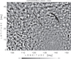 |
Fig. 1 A Dopplergram after removing the Carrington rotation and the 5-min oscillations. The position of the solar disk center (white cross) for August 23, 2000, at 9:30 UT is 137.1° in heliographic longitude and 7.0° in latitude. Scale in ms−1.The image shows exactly the region within the white solid lines in Fig. 2. |
2.2 Hα observations
Full disk chromospheric observations in Hα line from KSO and Big Bear Solar Observatory (BBSO) were used. The KSO images were observed using a telescope with a diameter of 100 mm and a Lyot Hα filter (full width at half maximum (FWHM) = 0.7 Å); more details about the telescope can be found in Veronig & Pötzi (2016). The images are suitable for the determination of the positions of filaments, plagues, and active regions. The telescope at BBSO has a higher resolution (diameter of 150–200 mm) and a very narrow filter with a FWHM of0.25 Å (more details in Denker et al. 1999). While images from BBSO have a very good angular resolution and are suitable for the identification of details in the chromosphere, filament channels, and in filaments (Fig. 2), the images from KSO have the advantage of being taken with the same cadence at the same time.
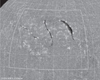 |
Fig. 2 A Hα image from August 23, 2000, at 15:56 UT taken at BBSO. It shows the selected region labeled as No. 1 in Table 1 with well developed filaments. Small white circles indicate the end points of the barbs of filaments. The solid white lines are the borders of the region where the horizontal velocities were calculated. |
3 Methods
3.1 Horizontal velocity fields from Dopplergrams
In order to obtain the velocities at first from each Dopplergram, the rigid Carrington rotation profile has to be removed and the signal from the 5-min oscillation. To eliminate these oscillation signatures, a filter suggested by Hathaway (1988) was applied:
![Mathematical equation: \begin{equation*} F^{n}[V(t)]= \sum_{j=0}^{n} \left( \frac{1}{2^{n}} \frac{n!}{j!\:(n-j)!} \right) V(t_{0}+ j \mathrm\Delta t).\end{equation*}](/articles/aa/full_html/2018/05/aa31162-17/aa31162-17-eq1.png) (1)
(1)
For our purpose, we applied the so-called weighted comb filter, that is, a series of n = 14 measurements of the Doppler velocity field V (t) with a sampling interval of Δt = 120 s and a temporal length of 28 min. A Fourier analysis of the resulting Dopplergrams no longer shows a periodic signal.
The aim is to obtain horizontal velocities as a continuous vector array over the whole studied region. For this purpose the most convenient structures are the convection elements which are continuously displaced in the photosphere. In our case we prefer the structures with the size of supergranules that have lifetimes of at least one day. The measured Doppler velocities represent the radial plasma velocity in the photosphere seen from the viewpoint of the observer. Since the horizontal velocities in supergranules are dominant, the area around the center of the solar disk has almost no Doppler signal, while with increasing central meridian distance the radial velocities also increase, which can be seen very clearly in Fig. 1.
The LCT method, described in detail by November (1986) is a useful tool to obtain velocities in the solar photosphere. The resolution of the method is governed by setting a window size for obtaining correlation values between two subsequent frames. In our work we used a window size of 1.5° and additionally 3° and 4.5° for testing purposes. When the LCT procedure is applied on two Dopplergrams with a time separation of Δ t, the resulting map provides a displacement map of the convection structures. The displacement is simply proportional to the horizontal velocity field. Displacement does not directly relate to the local small-scale plasma velocity, but to the velocity with which the convection cells change their shape or size and how they migrate horizontally. For each different heliographic latitude in the orthogonal coordinate system the displacement vector was remapped into the correct real value of the zonal velocity.
The Dopplergrams which we use for the LCT method are averaged over almost half an hour, the time separation between two Dopplergrams in the LCT analysis is at least 2 h (see Eq. (1)). For each selected day, spanning about 8–10 h of observations, we obtain about ten velocity maps.
The resulting horizontal velocity field depends strongly on the convolution window size of the LCT method, which is proportional to the resulting spatial resolution of the velocity field. Additionally the convolution window size acts like a spatial averaging of the velocity vectors and lowers the modulus of velocity vectors generally. The typical structure of the horizontal velocity field derived from our observing materials at the maximum achievable spatial resolution is shown in Fig. 3. Another effect is the increase in size of the resulting cells with the window size, which was also mentioned in Hindman et al. (2006); Roudier et al. (2008) and Schmieder et al. (2014).
A very demonstrative tool to visualize the characteristics of a velocity field is a corkmap, whereby artificial test particles, corks, are moved within the velocity field (November et al. 1987). At the beginning the corks are distributed uniformly over the velocity field. Then they are moved along the velocity vectors frame by frame. After a while one can see that the corks move to the cell borders, then they move along these cell borders and begin to clump together in locations of maximum convergence (see Figs. 3–5). The cork density forms the cell pattern, where the cells commonly form a simple closed formation and are sometimes partially open. In many cases there is a connection of several cells with a single closed boundary.
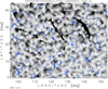 |
Fig. 3 Area No. 1 from Table 1 as velocity field overlaid with corks (blue), both from LCT methods applied on Dopplergrams in the interval from 7 UT to 10 UT on August 23, 2000, and filaments from KSO Hα observed at 8:23 UT. The blue corks gather at areas with high convergence of the velocity field. The scaling vector of the velocity field is shown in the lower-left corner. In the upper-right corner a circle with a cross shows the size of the convolution window for the LCT method (i.e., the LCT resolution). The small rings near the filaments indicate the locations of the barbs. |
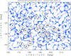 |
Fig. 4 A corkmap showing the velocity cells in the time interval from 5:31 UT to 9:30 UT on July 28, 2002. The labeled circles are for comparison of cell boundaries and their evolution with those in Fig. 5. |
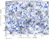 |
Fig. 5 As in Fig. 4 but at a later time interval (9 UT to 13 UT). The square in the top-left corner shows the size of the averaging window. |
3.2 Axial and transversal velocities below the filaments
The main objective of this work is to study the velocity distribution in the vicinity of filaments. From direct measurements, we did not find that the velocity field below and around the filaments has any unique structure for the case of the presence of a PIL. An important finding is that end points of barbs correlate well with the locations of high local convergence of the velocity vectors. The analysis of the velocity profile for axial and transverse velocities was performed for all of the 16 selected areas (Table 1). Each area comprises at least four quiescent filaments on both hemispheres for the years 2000 and 2002.
For eachregion, two velocity fields were produced with a time difference of 2 h and an average over several hours for increasing the S/N. Mean velocities were derived from temporally equally spaced measurements made in morning hours of each day over a period of three days and covering a time interval of nearly 57 h. In order to study the velocity field on both sides of the PIL, we created rectangular test boxes along the filament axis (see Fig. 6). The test boxes are drawn in white, led by the arrowhead in the direction of the box axis and margined on the right side with triangles and on the left side with circles. The size and position of the test box is selected so that the start and end points of the axis will follow the PIL or locations where legs of the filament are anchored in the photosphere. In some cases it is difficult to find the exact location of these legs.
The measurement method was as follows: The rectangular test box of size [n,2m] oriented along the axis of the filament was equally divided into n = 22 and m = 50 points on both sides. For these 2200 locations the velocity vectors were obtained and split into a component along the test-box (filament) axis v∥ and perpendicular to the axis v⊥. Finally, for both components, v∥ and v⊥, we separately calculate the average values from 22 points for all m = 50 different distances on both sides of the axis. Thereby we obtained the mean values  and
and  . For the dependence of the average value of the distance from the axis of the box we use the term axial or transverse average velocity profile.
List of all filaments measured in the 2 years, 2000 and 2002.
continued.
3.3 Filament chirality and shearing motions
Determination of the chirality of the 64 filaments was done using the methodology suggested by Martin et al. (1992) using the inclination of the threads of the filaments observed in Hα images from BBSO. Dextral filaments are characterized using a simple rule: viewing from the positive polarity of the bipolar magnetic region, the threads and barbs of the filament are directed to the right side from the filament axis. This is the case when the axial velocity of the plasma flow on the side of negative polarity is oriented towards the left side and the axial flow on the other side is slower or is in the opposite direction. For sinistral filaments the situation is reversed. An example for dextral filaments is in Fig. 2 with the corresponding magnetic map in Fig. 6; the sinistral type can be seen in Figs. 7 and 8.
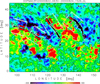 |
Fig. 6 Measurements of the average axial velocities near four filaments on August 22–24, 2000. Filaments are shown as black profiles with white borders. The white test boxes are oriented along the projected line of anchoring feet of the filaments. On both sides of the axis are white dotted lines along which the average values of the axial velocities were calculated. The velocity ratio is shown by two thick red arrows, whose lengths are proportional to the velocity difference, which is also shown as an inclined black dashed line. |
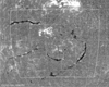 |
Fig. 7 The Hα image from BBSO of region No. 13 (Table 1) from January 9, 2002, taken at 18:41 UT. Small white circles indicate the end points of the barbs of the filaments. White lines are borders of the region, where the horizontal velocity field was calculated. |
4 Results
4.1 Horizontal velocity fields
A Dopplergram consists of radial velocity cells, moving towards the observer ( positive/bright) or away from them (
 negative/dark) as can be seen in Fig. 1. The size of these cells is in the range of 11.5–14 Mm. The cells of the same orientation often coalesce and form a continuous string with lengths up to ten times that of the cell size. Figure 9 shows the distribution of the cell sizes. The smallest visible features in Dopplergrams are around 2° ( ~25 Mm) near the solar equator. These cells are persistent over 3–4 h, however at the same time the elements can slowly change brightness, move in the zonal and meridional direction, and vary their size and shape. These changes are thought to result from the velocity field in the convective cells, which we are not able to measure in greater detail due to lack of resolution.
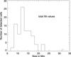 |
Fig. 9 Histogram of the cell size measured on the Dopplergrams after removing p-mode oscillations and the Carrington rotation. |
4.2 Horizontal velocity patterns and their characteristics
Figure 10 shows the frequency distribution of the horizontal velocities derived from Fig. 3. While the most frequent velocities are in the range of 110–220 ms−1, the average horizontal velocity is 262 ms−1. Whereas theaverage horizontal velocity values were calculated over a 240-min time interval for Fig. 10, for all areas listed in Table 1 the values were averaged over a few days, so the average value is lower. The average for all eight time intervals is 143 ms−1 and the median is 119 ms−1. The asymmetric velocity profile has a geometric source; the smallest horizontal velocities are in the center of the convection cells, while the higher velocities are observed at the periphery covering a larger area than the central region.
As a test of the stability of the cells they were marked with numbers (Fig. 4) and compared to the pattern after 3 h. Almost all cells can be found again in Fig. 5. They are only shifted by about 0.1–0.6 circle diameters and in four casesthey even kept their position. In Fig. 5 the large scale velocity field vectors are added and the size of the averaging window is marked in the top left corner. This large-scale velocity field moves and probably deforms the cells. Relationship among the cork density lines (cells boundaries), the magnetic field in photosphere, filaments silhouettes and detected barbs is shown in Fig. 11. The difference between the velocity field generating the cells and the large-scale field is also visible in Figs. 12 and 13.
The cells in the horizontal velocity field maps are due to the supergranular convection. The resolution of our data is near the lower limit for the detection of such cells with the LCT method, as a minimum window size of 3 pixels is needed. The resulting cell sizes, however, are in good agreement with the generally accepted dimension of supergranular cells of about 25–40 Mm (Fig. 14). The borders between these cells are places with the highest convergence of the horizontal flow; normally these regions coincide with places of concentrated magnetic flux (Roudier et al. 2016). It is obvious that centripetal flow exists in these regions and thus towards the PIL if itlies close to them. At higher resolution the PIL is not a smooth straight line, in fact it significantly meanders, which has its origin in the supergranular convection cells, which are driven towards the axis of the filament.
The large-scale velocities found in all areas describe the differential rotation and meridional circulation of the solar plasma. Ambrož & Schroll (2002) noted that these velocities alone may be the reason for shifting filaments as a whole or their parts, which may be interpreted as the proper motion of the filaments. Similarly, it is possible that anomalies in differential rotation of the filaments (pivot-points), which in the past have been revealed by Mouradian et al. (1987), are intervening solely with this type of flow or movement. As an important result of this section, we consider that horizontal velocities create cellular structures, where the largest horizontal velocities dominate at the location of the cell boundaries. In these places there is also the maximum convergence of horizontal flows. Cells retain their identity for at least 3 h and therefore the changes in their position are influenced by a large-scale advection.
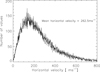 |
Fig. 10 Distribution of the horizontal velocities derived for August 23, 2000, between 7 UT and 10 UT. |
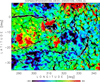 |
Fig. 11 AreaNo. 13 from Table 1 on the southern hemisphere as an overlay of corks on the magnetic field (in color) on January 9, 2000, from 8:303 UT to 12:59 UT. The small circles near the black filament’s profile indicate the endpoints of the barbs. The magnetic field scale is in Gauss. |
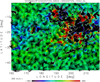 |
Fig. 12 Horizontal velocity distribution near the resolution limit of our observations for region No. 15 in Table 1 on July 29, 2002, from 6:02 UT to 10:42 UT. The velocity vector distribution is the same in the vicinity of filaments and far from the PIL in central parts of magnetic concentrations, which are shown as colored background. |
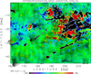 |
Fig. 13 The identical region as in Fig. 12 for the same time interval. In the large-scale velocity field (averaging window size in top-left corner) the axial component near the filaments is more remarkable than the transversal component. |
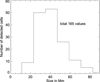 |
Fig. 14 Distribution of the diameter of the horizontal velocity cells obtained at highest possible resolution. The most frequent diameter lies in the range of 25–40 Mm, that is, the size of supergranular cells. |
4.3 Horizontal divergence and filament barbs
Locations with high cork densities were compared with the location of barbs in plots like Figs. 3 and 11. Barbs end far from the filament axis and dominate the silhouette of filaments; they seem to represent the feet, where the filament is anchored in the photosphere. There are several barbs located on both sides along each filament. Due to 3D effects some bards are sometimes not visible. The ends of the barbs near the photosphere are very narrow and thus below the resolution of our observational data. Another limiting factor is that the determination of anchoring of the barbs in thephotosphere can be a problem, as shown by Lin et al. (2005) with observations at much higher spatial resolution. The filament body itself is also not homogeneously massive, it consists of thin threads or fibrils, which are inclined to the filament axis and are directed from one side of the PIL to the other. Therefore in some cases we cannot eliminate the possibility that a bold thread can be considered as a barb, which extends into the photosphere.
The positions of the ends of the barbs were studied in the areas 1 (Table 1, August 22, 2000), 5 (Table 1, October 24, 2000) and 13 (Table 1, January 9 and 10, 2002). A total of 71 barb ends were detected; out of them 55% were directly anchored in locations of high cork densities, 30% in the close vicinity, and only in 15% the barb ended outside. The last case may be due to the fact that the barb ends are very difficult to detect, especially at this resolution. Nonetheless the agreement between areas with high convergence of horizontal velocities and the ends of the filament barbs in the photosphere is very good.
4.4 Axial and transversal velocities below the filaments
The orientation of the axial velocity in Fig. 6 is always positive in the direction of the arrow on the front of the box. The transverse velocity is positive in the direction from the circles to the triangles (left to right). On both sides of the axis within the box, there is a dashed line, where averaged velocities are compared. The distance of the lines from the axis is 0.94 heliographic degrees. It corresponds to a mean distance between 9 and 11 Mm depending on the heliographic latitude. Both lines are a limiting belt which is only 20 Mm broad and restricts thearea of the filament channel below the filament. Values obtained on these distances are labeled as  and
and  describing axial or transversal average velocities.
The axial velocity differences on both sides of the filament axis are shown as large red arrows in Figs. 6 and 8. The length of both is proportional to their magnitude and is simply for mutual comparison. Both arrows represent how different the velocities  and
and  are for creation of the bold black dashed line. The structure of the chromosphere and filaments as well as the position of the barbs for region No. 13 (Table 1) of January 9, 2002, is illustrated in Fig. 7.
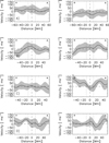
A broader range of the velocity profiles of the mean values of axial and transverse velocity can be seen in Figs. 15 and 16, where variations of the mean velocity are on average in the range of about 100–150 ms−1. The profile of values are varying within the range of the test box and usually the changes are not sudden, but in many cases the average speed varies almost periodically. In Fig. 15 the shortest length of the period is about 15–20 Mm (profile B) and the longer periods are about 40 Mm (section A). Sometimes there is a continuous change from one side of the box to the other in the range of about 90 Mm (section C). In many cases, the short term changes modulate the long-period profile (section D). Also in Fig. 16 similar variations were found as well as in all other cases of our observations.
The difference  is calculated as a mean value from all measurements taken for the entire observing interval, which is usually three or four days at a distance of 10 Mm from the filament. The value is positive if the right and left sides relate to the direction of the magnetic field in the axis of the filament. The gradient of velocity at this base is
  , which is shown in the seventh col. of Table 1. Similarly, the average value of the divergence in the direction perpendicular to the axis of the filament for all the measurements was determined as
  (last col. in Table 1). The gradient of the axial velocity directly relates to the shearing movement of plasma on both sides of the filaments, and the average values of divergence correlate with the transversal divergence or convergence.
In all 16 cases there exists a difference between the average velocities of the left side of the filament and the velocities on the rightside, that is a shear movement. This shear movement can be a reason for the transformation from originally current-free magnetic field with a dominant vector perpendicular to the PIL into a magnetic configuration, where the axial component of the magnetic field dominates. The arcs are anchored on both sides of the PIL in opposite polarities. Due to shearing motion of magnetized plasma on both sides of the PIL this can lead to a deformation of the arc and a gradual rotation of their plane to that of the axis of the filament. This is a process that would transform the original potential-structure perpendicular to the PIL to a configuration, which has the main component of the magnetic vector oriented along the axis of the filament. This mechanism is discussed by Rompolt & Bogdan (1986).
The absolute value of the gradient in all studied cases is varying in a broad range from 0.06 to 5.49. It is very difficult to find a relationship between the gradient value and the angle between the threads and the axis inside the filament. With this dataset this cannot be measured. Our results do support the hypothesis that the deformation of the current free (potential) magnetic field lines is caused by the shearing motion on both sides of the axis of the filament. In this case the correlation between the thread orientation inside the filament and the gradient of axial velocities must be reasonable. A quantitative comparison cannot be made due to the duration of deformation, the lifetime of the deformed structures, and their ability to relax.
Based on all of our measurements, we can say the following: All axial velocities show a shear axial movement relative to the PIL and thesize of the shear varies. Also, transverse rates were detected in all cases, and the rates of convergent and divergent flow were statistically comparable.
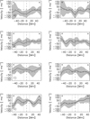 |
Fig. 15 Graphical representation of mean axial |


4.5 Filament chirality and shearing motions
The numberof the studied areas in Table 1 is the same for both solar hemispheres. A determination of the chirality was possible for 62 cases; 40 (64.5%) of them were dextral and 22 (35.5%) sinistral. In the northern hemisphere 28 (90%) of 31 filaments are of the dextral type, and in the southern hemisphere 20 (62.5%) out of 32 are sinistral. For each analyzed filament, the average divergence relative to the axis of the filament was also calculated (last col.), but there is no significant trend visible, the positive values (37 cases, 57.8%) dominate.
Much more important than the numerical value of the gradient is the comparison of the chirality of the filament with the orientation of the gradient of the axial velocity ( ). The question here refers to whether the horizontal speed is able to cause shearing of the chromospheric loops or arches due to the motion of the footpoints. The total number of 62 compared measurements showed an agreement in 57 (92%) cases, a disagreement in 4 cases and in only one case the gradient was negligible. This gradient describes the different velocity of two points parallel to the PIL at a distance of about 20 Mm. This movement increases the distance between these points, which means that the angle of the fibers to the filament axis decreases with time.
On the basis of simple geometry it can be said that an angle of 5° between the axis of the PIL and a fiber is reached after 66, 33, or 22 days at a gradient ( ) of 2, 4, or 6. This time can be considerably shortened if the relative lateral velocities are convergent. Given that our measurement interval time scale did not exceed 4 days, the above-mentioned time intervals are incomparably longer and further measurements are needed to determine whether or not the found gradient velocity is persistent in the long-term. As many quiescent filaments have live times of a few solar rotations and the gradient of fiber orientation in all our entire set is in good agreement for many stages of the filament evolution, we consider, with a high probability, that this property is persistent in time.
Figure 17 shows the gradient ( ) in relation to the heliographic latitude of the measured filaments. The lowest gradient values occur also near the equator, while the largest (extreme) values are found for filaments in higher latitudes than 20°. The dashed line represents the calculated dependence of the velocity gradient for the differential rotation curve on the heliographic latitude from Eq. (A.1) using the coefficients B and C according to Table A.1 for k = 3.8 specified in Appendix A. Although the measured filaments do not have purely zonal (parallel to the equator) orientation, it can be assumed that a substantial portion of the axial velocity component can be influenced due to the mean zonal velocity, which is dependent on the heliographic latitude. To summarize we can say that the orientation of the mean shear movements in almost all the cases studied has the same orientation as the derived chirality of the fibers in the filaments.
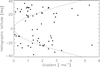 |
Fig. 17 Gradients ( |

5 Conclusions
The main results of our analysis of the surface horizontal flow below the filaments can be summarized as follows:
Horizontal velocities were determined by comparing pairs of temporally different Dopplergrams of supergranular convection by using the LCT method. The velocity field in all selected areas shows characteristic cells, in which the vector field is oriented from the center to the border of the cells. The typical mean cell size is between 25 and 40 Mm and the mean velocity derived by this method lies around 200 ms−1. The location of the cells is relatively stable and varies during one day only within half of a cell size. High convergence is characteristic for the boundary of the cells and the divergence is negative as confirmed with corkmaps.
The horizontal velocity field has a significant relationship with the filaments, especially in places where filaments/prominences are anchored in the photosphere. The places in the photosphere at which the projected end points of barbs are located coincide very well with areas of maximum convergence of the velocity field.
Investigating the horizontal velocity of cells in close proximity to and below the filament (thus in filament channel) shows that velocity cells may indicate a flow across the PIL, but also in locations along the PIL. The structure of horizontal cells does not change significantly in the vicinity of the filaments or beneath them, as well as at greater distances from the filament.
Filaments are formed along the mean PIL and have a straight or slightly curved shape. Measurements of average velocity on both sides of the filament confirm that in all cases a transverse gradient of the axial velocity below the filament was detected. The axial velocity gradient varies for different filaments. The difference of the longitudinal velocity in all measured cases with few exceptions (6.45%) corresponds with the fibrils inclination and their orientation in a filament.
The average transverse velocity does not show any correlations. This result refers to the calculated average values of the transverse velocities always along the entire measured section of the filament. This means that the assumption of homogeneous transversal flow across the entire section on both sides of the filament was not confirmed by our measurements. It cannot be concluded from our measurements that there is a continuous oriented flow either to the filament axis or vice versa along the entire length of a filament.
In all cases around the filament, the horizontal velocities are broken down into the cellular structures at whose borders there is the highest convergence. These boundaries, in many cases at the common borders of several cells, form the nucleus of convergence, or end points of convergent lines, respectively. Such places in the vicinity of the filament coincide very well with the legs of the filaments (barbs). Converging lines represent trajectories and geometric locations that are highlighted by supergranular turbulence, that is, where the test particles move from the center of the cells to the concentration nuclei. This structuring shows that on both sides of the filaments are locations where convergent lines are. On both sides we observe the far larger areas where horizontal velocities dominate, but the magnetic flux is insignificant. Converging regions show far lower horizontal velocities than the areas around them, but they are associated with increased magnetic flux intensity. Magnetic flux transfer then proceeds from the center of the magnetic field of the respective polarity to the neutral line of the PIL, where it effectively annihilates with the magnetic flux of the opposite polarity. The speed of this transport is difficult to determine, because our velocity field represents an immediate (or in a short interval) pattern, while this transport is a process in which the position and shape of the cells change continuously over a much longer time span.
The presence of the gradient axial velocity and its very good agreement with the fiber orientation (chirality) in the filaments is a reason to suppose that the transformation of current-free magnetic field to a field with significant axial component is caused by the presence of the axial velocity in the photosphere and their influence on the anchors of the magnetic structure in the vicinity on both sides of the PIL.
The averaged values of the horizontal velocity can be used as a complementary profile of the solar differential rotation. In the latitude profile of the zonal velocity we found significantly lower values than previously proposed by many other authors. For scaling of our measurements, we used a multiplication factor of k = 3.8 for all partial measurements; in this case we get very good agreement.
Acknowledgements
Authors acknowledge the following institutions for making this work possible: Big Bear Solar Observatory/New Jersey Institute of Technology; Department of Physics, University of Rome “La Sapienza”, Italy; Trieste Astronomical Observatory, Trieste, Italy and Kanzelhöhe Observatory for Solar and Environmental Research, University of Graz, Austria. A special thanks goes to the former coworkers ofthe KSO T. Pettauer, A. Schroll and W. Otruba, who were involved during the years 2000–2002 in the development of the MOF and the daily observations.
Appendix A: Zonal velocity test
The velocities derived with the LCT method most likely do not correspond to true horizontal velocity due to systematic underestimation due to the convolution windows having a finite dimension. The zonal velocity components in the measured areas were used to test the degree of this degradation. Since the zonal measurements obtained should correspond to the differential rotation, we applied a multiplication factor k to our measurements.
Differential rotation coefficients.
Calculations of the horizontal velocities are performed in a segment of the solar disk between ± 60 heliographic degrees in latitude and a width of 90° in heliographic longitude. In this area the mean values for zonal and meridional velocity components are obtained. The velocity values are averaged for each observing day and then combined for the time span of each observation set. The zonal velocities were not corrected for differential rotation. It should be noted that the results from the meridional component vary quite significantly.
Figure A.1 combines mean values of zonal velocity from the time periods September 10–13, 2000, August 25–28, 2001,and July 28–31, 2002. The average value of the zonal velocity relative to Carrington coordinate system is drawn with a thin solid line overlapped with bold dashes, the standard deviation is marked as light gray area. The fitted curve can be expressed using Fay’s formula, that gives the relation between angular velocity and heliographic latitude ϕ:
 (A.1)
where the coefficients A, B, and C are normally given in ms−1 like in Fig. A.1 or in μrad s−1 as in Table A.1, where also corresponding values of other authors are presented for comparison. The values of the coefficients in Table A.1 are varying only in a small range. The most precise measurements were done with recurrent spots in the solar photosphere (e.g., Newton & Nunn 1951), while for the magnetic field they are somewhat lower and for the Doppler velocity the uncertainty is the highest.
(A.1)
where the coefficients A, B, and C are normally given in ms−1 like in Fig. A.1 or in μrad s−1 as in Table A.1, where also corresponding values of other authors are presented for comparison. The values of the coefficients in Table A.1 are varying only in a small range. The most precise measurements were done with recurrent spots in the solar photosphere (e.g., Newton & Nunn 1951), while for the magnetic field they are somewhat lower and for the Doppler velocity the uncertainty is the highest.
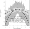 |
Fig. A.1 Combining several graphs of the differential rotation profiles depending on heliographic latitude obtained from the sources that are listed in Table A.1. The light gray area is the standard deviation for the case k = 1 and the darkgray area for k = 3.8. |
Our measurements are performed in the photosphere and can be therefore compared with measurements by Snodgrass (1983) and with the classic measurement of recurrent sunspots by Newton & Nunn (1951). The comparison (Fig. A.1) shows that our measurements are much lower towards higher latitudes than the above mentioned ones. A reason for this deviation is probably the systematic underestimation of the speeds due to the LCT method when using a window size of 1.5° (and therefore lower spatial resolution) during calculation of the horizontal velocity. Therefore the real horizontal speed in the photosphereis probably higher than in our measured cases. We found average values for the horizontal velocity in the range from 100 to 150 ms−1 whereas measurements at higher spatial resolutions lead to values in the range from 300 to 640 ms−1 (Roudier et al. 1999; Krijger et al. 2002; Lin et al. 2005).
The best fit of our curve with the curve of differential rotation obtained for doppler velocities by Snodgrass (1983) can be achieved when all our measurements are multiplied by the factor k = 3.8. From this, we assume that this is the factor for which all LCT-derived horizontal velocity values were underestimated against the real values. In Fig. A.1 the thick solid line shows the mean differential profile for k = 3.8 together with the standard deviation as gray area. These values, however, differ a lot from corona measurements made by Trellis (1957) and Sýkora (1994) using data from Pic du Midi and Lomnický štít or Fisher & Sime (1984) with Mauna Loa data. But these coronal measurements suffer from great uncertainty of the determination of the positions of brightenings. New space-borne data of the coronal objects observed in EUV radiation are of much better resolution and they do not show any systematic deviation of the rotation velocities between the corona and photosphere in latitudes above 15° (Wöhl et al. 2010). This we consider as a strong argument for co-rotation of significant coronal structures with strong magnetic fields in the photosphere.
References
- Amari, T., Luciani, J. F., Mikic, Z., & Linker, J. 1999, ApJ, 518, L57 [NASA ADS] [CrossRef] [Google Scholar]
- Amari, T., Luciani, J. F., Mikic, Z., & Linker, J. 2000, ApJ, 529, L49 [NASA ADS] [CrossRef] [PubMed] [Google Scholar]
- Ambrož, P., & Schroll, A. 2002, A&A, 381, 300 [NASA ADS] [CrossRef] [EDP Sciences] [Google Scholar]
- Cacciani, A., & Fofi, M. 1978, Sol. Phys., 59, 179 [Google Scholar]
- Cacciani, A., Ricci, D., Rosati, P., et al. 1990, Il Nuovo Cimento C, 13, 125 [Google Scholar]
- Cacciani, A., Comari, M., Furlani, S., et al. 1998, in Three-Dimensional Structure of Solar Active Regions, eds. C. E. Alissandrakis, & B., Schmieder ASP Conf. Ser., 155, 265 [NASA ADS] [Google Scholar]
- Denker, C., Johannesson, A., Marquette, W., et al. 1999, Sol. Phys., 184, 87 [NASA ADS] [CrossRef] [Google Scholar]
- DeVore, C. R., & Antiochos, S. K. 2000, ApJ, 539, 954 [NASA ADS] [CrossRef] [Google Scholar]
- Engvold, O. 2015, in Solar Prominences, eds. J.-C. Vial & O. Engvold, Astrophys. Space Sci. Lib., 415, 31 [NASA ADS] [CrossRef] [Google Scholar]
- Fisher, R., & Sime, D. G. 1984, ApJ, 287, 959 [NASA ADS] [CrossRef] [Google Scholar]
- Foukal, P. 1971a, Sol. Phys., 20, 298 [NASA ADS] [CrossRef] [Google Scholar]
- Foukal, P. 1971b, Sol. Phys., 19, 59 [NASA ADS] [CrossRef] [Google Scholar]
- Gaizauskas, V., Zirker, J. B., Sweetland, C., & Kovacs, A. 1997, ApJ, 479, 448 [NASA ADS] [CrossRef] [Google Scholar]
- Hathaway, D. H. 1988, Sol. Phys., 117, 1 [NASA ADS] [CrossRef] [Google Scholar]
- Hindman, B. W., Haber, D. A., & Toomre, J. 2006, ApJ, 653, 725 [NASA ADS] [CrossRef] [Google Scholar]
- Krijger, J. M., Roudier, T., & Rieutord, M. 2002, A&A, 387, 672 [NASA ADS] [CrossRef] [EDP Sciences] [Google Scholar]
- Lin, Y., Wiik, J. E., Engvold, O., Rouppe van der Voort, L., & Frank, Z. A. 2005, Sol. Phys., 227, 283 [NASA ADS] [CrossRef] [Google Scholar]
- Mackay, D. H., Gaizauskas, V., & Yeates, A. R. 2008, Sol. Phys., 248, 51 [NASA ADS] [CrossRef] [Google Scholar]
- Mackay, D. H., Karpen, J. T., Ballester, J. L., Schmieder, B., & Aulanier, G. 2010, Space Sci. Rev., 151, 333 [NASA ADS] [CrossRef] [Google Scholar]
- Magara, T., & Kitai, R. 1999, ApJ, 524, 469 [NASA ADS] [CrossRef] [Google Scholar]
- Martin, S. F. 1990, in Lecture Notes in Physics, eds. V. Ruzdjak, & E. Tandberg-Hanssen, IAU Colloq. 117: Dynamics of Quiescent Prominences (Berlin: Springer Verlag), 363, 1 [NASA ADS] [CrossRef] [Google Scholar]
- Martin, S. F. 1998, in IAU Colloq. 167: New Perspectives on Solar Prominences, eds. D. F. Webb, B. Schmieder, & D. M. Rust, ASP Conf. Ser., 150, 419 [NASA ADS] [Google Scholar]
- Martin, S. F., & Echols, C. R. 1994, eds. R. J. Rutten, & C. J. Schrijver, NATO Advanced Science Institutes (ASI) Series C, 433, 339 [Google Scholar]
- Martin, S. F., Marquette, W. H., & Bilimoria, R. 1992, in The Solar Cycle, ed. K. L. Harvey, ASP Conf. Ser., 27, 53 [NASA ADS] [Google Scholar]
- Martin, S. F., Bilimoria, R., & Tracadas, P. W. 1994, eds. R. J. Rutten, & C. J. Schrijver, NATO Advanced Science Institutes (ASI) Series C, 433, 303 [Google Scholar]
- Moretti, P. F., & MOF Development Group. 2000, Sol. Phys., 196, 51 [NASA ADS] [CrossRef] [Google Scholar]
- Mouradian, Z., Martres, M. J., Soru-Escaut, I., & Gesztelyi, L. 1987, A&A, 183, 129 [NASA ADS] [Google Scholar]
- Newton, H. W., & Nunn, M. L. 1951, MNRAS, 111, 413 [NASA ADS] [Google Scholar]
- November, L. J. 1986, Appl. Opt., 25, 392 [NASA ADS] [CrossRef] [PubMed] [Google Scholar]
- November, L. J., Simon, G. W., Tarbell, T. D., Title, A. M., & Ferguson, S. H. 1987, eds. G. Athay, & D. S. Spicer, NASA Conf. Pub., 2483, 121 [Google Scholar]
- Rompolt, B., & Bogdan, T. 1986, ed. A. I. Poland, NASA Conf. Pub., 2442, 81 [Google Scholar]
- Rondi, S., Roudier, T., Molodij, G., et al. 2007, A&A, 467, 1289 [NASA ADS] [CrossRef] [EDP Sciences] [Google Scholar]
- Roudier, T., & Muller, R. 1986, Sol. Phys., 107, 11 [NASA ADS] [CrossRef] [Google Scholar]
- Roudier, T., Rieutord, M., Malherbe, J. M., & Vigneau, J. 1999, A&A, 349, 301 [NASA ADS] [Google Scholar]
- Roudier, T., Švanda, M., Meunier, N., et al. 2008, A&A, 480, 255 [NASA ADS] [CrossRef] [EDP Sciences] [Google Scholar]
- Roudier, T., Malherbe, J. M., Rieutord, M., & Frank, Z. 2016, A&A, 590, A121 [NASA ADS] [CrossRef] [EDP Sciences] [Google Scholar]
- Rust, D. M. 1967, ApJ, 150, 313 [NASA ADS] [CrossRef] [Google Scholar]
- Schmieder, B., Roudier, T., Mein, N., et al. 2014, A&A, 564, A104 [NASA ADS] [CrossRef] [EDP Sciences] [Google Scholar]
- Smith, S. F., Ramsey, H. E., & Howard, R. 1965, AJ, 70, 330 [CrossRef] [Google Scholar]
- Snodgrass, H. B. 1983, ApJ, 270, 288 [NASA ADS] [CrossRef] [Google Scholar]
- Sýkora, J. 1994, Adv. Space Res., 14, 73 [NASA ADS] [CrossRef] [Google Scholar]
- Tang, F. 1987, Sol. Phys., 107, 233 [NASA ADS] [CrossRef] [Google Scholar]
- Trellis, M. 1957, Suppl. Ann. Astrophys., 5, 3 [Google Scholar]
- van Ballegooijen, A. A., & Martens, P. C. H. 1987, ApJ, 343, 971 [Google Scholar]
- Veronig, A. M., & Pötzi, W. 2016, in Coimbra Solar Physics Meeting: Ground-based Solar Observations in the Space Instrumentation Era, eds. I. Dorotovic, C. E. Fischer, & M. Temmer, ASP Conf. Ser., 504, 247 [NASA ADS] [Google Scholar]
- Wöhl, H., Brajša, R., Hanslmeier, A., & Gissot, S. F. 2010, A&A, 520, A29 [NASA ADS] [CrossRef] [EDP Sciences] [Google Scholar]
- Xia, C., & Keppens, B. 2016, ApJ, 823, 22 [Google Scholar]
All Tables
All Figures
|
Fig. 1 A Dopplergram after removing the Carrington rotation and the 5-min oscillations. The position of the solar disk center (white cross) for August 23, 2000, at 9:30 UT is 137.1° in heliographic longitude and 7.0° in latitude. Scale in ms−1.The image shows exactly the region within the white solid lines in Fig. 2. |
| In the text | |
|
Fig. 2 A Hα image from August 23, 2000, at 15:56 UT taken at BBSO. It shows the selected region labeled as No. 1 in Table 1 with well developed filaments. Small white circles indicate the end points of the barbs of filaments. The solid white lines are the borders of the region where the horizontal velocities were calculated. |
| In the text | |
|
Fig. 3 Area No. 1 from Table 1 as velocity field overlaid with corks (blue), both from LCT methods applied on Dopplergrams in the interval from 7 UT to 10 UT on August 23, 2000, and filaments from KSO Hα observed at 8:23 UT. The blue corks gather at areas with high convergence of the velocity field. The scaling vector of the velocity field is shown in the lower-left corner. In the upper-right corner a circle with a cross shows the size of the convolution window for the LCT method (i.e., the LCT resolution). The small rings near the filaments indicate the locations of the barbs. |
| In the text | |
|
Fig. 4 A corkmap showing the velocity cells in the time interval from 5:31 UT to 9:30 UT on July 28, 2002. The labeled circles are for comparison of cell boundaries and their evolution with those in Fig. 5. |
| In the text | |
|
Fig. 5 As in Fig. 4 but at a later time interval (9 UT to 13 UT). The square in the top-left corner shows the size of the averaging window. |
| In the text | |
|
Fig. 6 Measurements of the average axial velocities near four filaments on August 22–24, 2000. Filaments are shown as black profiles with white borders. The white test boxes are oriented along the projected line of anchoring feet of the filaments. On both sides of the axis are white dotted lines along which the average values of the axial velocities were calculated. The velocity ratio is shown by two thick red arrows, whose lengths are proportional to the velocity difference, which is also shown as an inclined black dashed line. |
| In the text | |
|
Fig. 7 The Hα image from BBSO of region No. 13 (Table 1) from January 9, 2002, taken at 18:41 UT. Small white circles indicate the end points of the barbs of the filaments. White lines are borders of the region, where the horizontal velocity field was calculated. |
| In the text | |
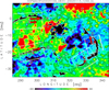 |
Fig. 8 As in Fig. 6 but for January 9–13, 2002. |
| In the text | |
|
Fig. 9 Histogram of the cell size measured on the Dopplergrams after removing p-mode oscillations and the Carrington rotation. |
| In the text | |
|
Fig. 10 Distribution of the horizontal velocities derived for August 23, 2000, between 7 UT and 10 UT. |
| In the text | |
|
Fig. 11 AreaNo. 13 from Table 1 on the southern hemisphere as an overlay of corks on the magnetic field (in color) on January 9, 2000, from 8:303 UT to 12:59 UT. The small circles near the black filament’s profile indicate the endpoints of the barbs. The magnetic field scale is in Gauss. |
| In the text | |
|
Fig. 12 Horizontal velocity distribution near the resolution limit of our observations for region No. 15 in Table 1 on July 29, 2002, from 6:02 UT to 10:42 UT. The velocity vector distribution is the same in the vicinity of filaments and far from the PIL in central parts of magnetic concentrations, which are shown as colored background. |
| In the text | |
|
Fig. 13 The identical region as in Fig. 12 for the same time interval. In the large-scale velocity field (averaging window size in top-left corner) the axial component near the filaments is more remarkable than the transversal component. |
| In the text | |
|
Fig. 14 Distribution of the diameter of the horizontal velocity cells obtained at highest possible resolution. The most frequent diameter lies in the range of 25–40 Mm, that is, the size of supergranular cells. |
| In the text | |
|
Fig. 15 Graphical representation of mean axial |
| In the text | |
|
Fig. 17 Gradients ( |
| In the text | |
|
Fig. A.1 Combining several graphs of the differential rotation profiles depending on heliographic latitude obtained from the sources that are listed in Table A.1. The light gray area is the standard deviation for the case k = 1 and the darkgray area for k = 3.8. |
| In the text | |
Current usage metrics show cumulative count of Article Views (full-text article views including HTML views, PDF and ePub downloads, according to the available data) and Abstracts Views on Vision4Press platform.
Data correspond to usage on the plateform after 2015. The current usage metrics is available 48-96 hours after online publication and is updated daily on week days.
Initial download of the metrics may take a while.