| Issue |
A&A
Volume 612, April 2018
|
|
|---|---|---|
| Article Number | A39 | |
| Number of page(s) | 12 | |
| Section | Cosmology (including clusters of galaxies) | |
| DOI | https://doi.org/10.1051/0004-6361/201731599 | |
| Published online | 19 April 2018 | |
A multi-instrument non-parametric reconstruction of the electron pressure profile in the galaxy cluster CLJ1226.9+3332
1
Institut de RadioAstronomie Millimétrique (IRAM),
38400
Grenoble, France
e-mail: This email address is being protected from spambots. You need JavaScript enabled to view it.
2
Laboratoire de Physique Subatomique et de Cosmologie, Université Grenoble Alpes, CNRS/IN2P3,
53 avenue des Martyrs,
38000
Grenoble, France
3
Imperial College London, Kensington,
London
SW7 2AZ, UK
4
Laboratoire Lagrange, Université Côte d’Azur, Observatoire de la Côte d’Azur, CNRS, Bvd de l’Observatoire, CS 34229,
06304
Nice Cedex 4, France
5
Laboratoire AIM, CEA/IRFU, CNRS/INSU, Université Paris Diderot, CEA-Saclay,
91191
Gif-Sur-Yvette, France
6
Astronomy Instrumentation Group, University of Cardiff,
CF10 3XQ, UK
7
Institut d’Astrophysique Spatiale (IAS), CNRS and Université Paris Sud,
91440
Orsay, France
8
Institut Néel, CNRS and Université Grenoble Alpes,
38042
Grenoble, France
9
Institut de RadioAstronomie Millimétrique (IRAM),
18012
Granada, Spain
10
Dipartimento di Fisica, Sapienza Università di Roma, Piazzale Aldo Moro 5,
00185
Roma, Italy
11
Univ. Grenoble Alpes, CNRS, IPAG,
38000
Grenoble, France
12
Aix-Marseille Université, CNRS, LAM (Laboratoire d’Astrophysique de Marseille) UMR 7326, 13388 Marseille, France
13
School of Earth and Space Exploration and Department of Physics, Arizona State University, Tempe,
AZ
85287, USA
14
Institut d’Astrophysique de Paris, Sorbonne Universités, UPMC Univ. Paris 06, CNRS UMR 7095,
75014
Paris, France
15
LERMA, CNRS, Observatoire de Paris, 61 avenue de l’Observatoire,
75014
Paris, France
Received:
19
July
2017
Accepted:
13
November
2017
Abstract
Context. In the past decade, sensitive, resolved Sunyaev-Zel’dovich (SZ) studies of galaxy clusters have become common. Whereas many previous SZ studies have parameterized the pressure profiles of galaxy clusters, non-parametric reconstructions will provide insights into the thermodynamic state of the intracluster medium.
Aim. We seek to recover the non-parametric pressure profiles of the high redshift (z = 0.89) galaxy cluster CLJ 1226.9+3332 as inferred from SZ data from the MUSTANG, NIKA, Bolocam, and Planck instruments, which all probe different angular scales.
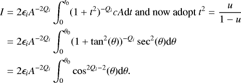
Methods. Our non-parametric algorithm makes use of logarithmic interpolation, which under the assumption of ellipsoidal symmetry is analytically integrable. For MUSTANG, NIKA, and Bolocam we derive a non-parametric pressure profile independently and find good agreement among the instruments. In particular, we find that the non-parametric profiles are consistent with a fitted generalized Navaro-Frenk-White (gNFW) profile. Given the ability of Planck to constrain the total signal, we include a prior on the integrated Compton Y parameter as determined by Planck.
Results. For a given instrument, constraints on the pressure profile diminish rapidly beyond the field of view. The overlap in spatial scales probed by these four datasets is therefore critical in checking for consistency between instruments. By using multiple instruments, our analysis of CLJ 1226.9+3332 covers a large radial range, from the central regions to the cluster outskirts: 0.05 R500 < r < 1.1 R500. This is a wider range of spatial scales than is typically recovered by SZ instruments. Similar analyses will be possible with the new generation of SZ instruments such as NIKA2 and MUSTANG2.
Key words: galaxies: clusters: individual: CLJ 1226.9+3332
© ESO 2018
1 Introduction
In recent years, Sunyaev Zel’dovich (SZ, Sunyaev & Zel’dovich 1970; Sunyaev & Zel’dovich 1972) effect observations have seen an increase in high resolution (θ≲30′′) observations (e.g., Mason et al. 2010; Adam et al. 2014; Kitayama et al. 2016). These observations come from MUSTANG on the Robert C. Byrd Green Bank Telescope (GBT; Dicker et al. 2008), NIKA on the IRAM 30-m telescope (Monfardini et al. 2010), and ALMA (band 3). However, all of these high resolution instruments have been limited in their ability to recover signal beyond their field of view (~ 45′′ for MUSTANG and ALMA, and ~ 120′′ for NIKA). As massive galaxy clusters at moderate redshift (z ~ 0.2−0.5) have characteristic radii, R500 ≳3′ 1, SZ observations made with these instruments have not been able to recover the entire signal of the observed galaxy clusters. Therefore, observations from complementary SZ instruments which recover SZ at larger scales such as Bolocam Czakon et al. (2015) or Planck (Planck Collaboration V 2013) have been used in join analyses by Romero et al. (2015) and Adam et al. (2015, 2016) respectively.
These joint analyses have shown the ability to constrain the pressure profile of the intracluster medium (ICM) of individual galaxy clusters over a large spatial range, often by assuming some parameterized pressure profile (e.g., Romero et al. 2017; Adam et al. 2014). In Romero et al. (2015), the differences in fitted pressure profiles, especially in additional constraint of the inner pressure profile slope, with the addition of MUSTANG data were noted. In the case of Romero et al. (2017); Adam et al. (2015, 2016), the pairs of instruments used had no overlap in recovered spatial scales, thus limiting the ability to ascertain systematic errors of instruments. However, as new SZ instruments like NIKA2 (Monfardini et al. 2014; Calvo et al. 2016) and MUSTANG2 (Dicker et al. 2014) with the ability to recover a larger range of scales come online, there will be overlap. Consequently, for clusters observed with multiple instruments (operating at different frequency bands), studies of the kinetic SZ effect, or relativistic corrections (Itoh et al. 1998) will be of significant interest and stand to benefit fromthe additional frequency coverage. The additional frequency coverage will help with removal of contaminants (e.g., compact sources), as well as offering additional leverage of the spectral distortion. To be sure of the results of these analyses, it will be critical to understand any systematics involved with individual instruments. Recent results combining Bolocam and Planck data (Sayers et al. 2016), which overlap in spatial scales recovered, show non-trivial changes (primarily of the outer slope of the pressure profile) from previous Bolocam-only results (Sayers et al. 2013).
Over a decade ago, the beta model (Cavaliere & Fusco-Femiano 1978) was favored; more recently other parameterizations such as a self-similar (Mroczkowski et al. 2009) and analytic pressure profile based on a polytropic equation of state (Bulbul et al. 2010) have been explored. Of the parameterizations of the ICM pressure profile, the generalized Navarro-Frenk-and-White (gNFW Nagai et al. 2007) profile has garnered the most traction, with a fairly canonical set of parameters coming from Arnaud et al. (2010; hereafter, A10), which used a sample of 33 local (z < 0.2) clusters. Recently, in several SZ studies non-parametric pressure profiles have been reconstructed either through a maximum-likelihood approach (e.g., Ruppin et al. 2017; Sayers et al. 2013) or through deprojection of deconvolved data (e.g., Basu et al. 2010; Sayers et al. 2011). The method employed in this paper maximized the marginalized posterior distribution,where the principle difference is our employment of analytic integrals.
Galaxy cluster formation is understood currently in the framework of hierarchical structure formation (e.g., Press & Schechter 1974). While remarkable that a simple self-similar treatment of clusters (Kaiser 1986) should describe the broad population of galaxy clusters, non-linear physical processes in cluster formation (see Kravtsov & Borgani 2012 for a review) likely account for much of the scatter in scaling relations (e.g., Battaglia et al. 2012). In this context, investigating cluster pressure profiles non parametrically can reveal deviations from a smooth pressure profile, which may correspond to departures from self-similarity (Basu et al. 2010). Moreover, these non-parametric fits do not rely on any physical model, and thus provide a less biased avenue to constraining the thermodynamic state of the ICM. The combination of non-parametric SZ pressure profiles with complementary non-parametric X-ray products, especially electron density, has (e.g. Basu et al. 2010; Planck Collaboration V 2013; Ruppin et al. 2017) and will provide insights into the thermodynamic state of the ICM in clusters and likely be fundamental for improving cosmological constraints via scaling relations. In fact, this is a significant motivation behind the NIKA2 tSZ large program (Comis et al. 2016), a 300 h program, using guaranteed time, to observe 50 homogeneously selected clusters at z≳0.5.
Counts of galaxy clusters by mass and redshift serve to constrain cosmological parameters, notably the dark energy density (ΩΛ), matter density (Ωm), the amplitude of matter fluctuations (σ8), and the equation of state of dark energy (w) (Planck Collaboration XXIV 2016). Constraints on these parameters derived from galaxy cluster samples are generally limited by the accuracy of mass estimation of galaxy clusters (e.g., Hasselfield et al. 2013; de Haan et al. 2016). Scaling relations which relate global (integrated) observables to the cluster mass are often employed. Currently, scaling relations as applied to observables over an intermediate radial region (R2500 ≲ r ≲ R500) of galaxy clusters is preferred as this range shows minimal scatter in the scaling relations (e.g., Kravtsov & Borgani 2012). This is due to the generally low cluster-to-cluster scatter in pressure profiles, found observationally and in simulations, within this radial range (e.g., Borgani et al. 2004; Nagai et al. 2007; Arnaud et al. 2010; Bonamente et al. 2012; Planck Collaboration V 2013; Sayers et al. 2013). While the relative homogeneity of pressure profiles in the intermediate region is well evidenced, it remains important to develop methods to derive non-parametric pressure profiles of clusters so that physical deviations are not artificially smoothed by the adoption of a parametric profile.
The use of observables quantities determined at intermediate radii motivates the inclusion of instruments which are able to recover the SZ signal out to these radii, while the need to recover deviations from a smooth profile favor higher resolution instruments. In order to then cover a wide range of angular scales (0.05 R500 < r < 1.1 R500), we have performed fits on MUSTANG, NIKA and Bolocam data, with the addition of a prior from Planck data. This paper is organized as follows. In Sect. 2 we review the NIKA, MUSTANG, and Bolocam observations and reduction. In Sect. 3 we address the method used to non-parametrically fit pressure profiles to each of the data sets. We present results from our non-parametric fits in Sect. 4 and parametric fits in Sect. 5. Throughout this paper we assume a ΛCDM cosmology with Ωm = 0.31, Ωλ = 0.69, and H0 = 68 km s−1 Mpc−1, consistent with the cosmological parameters derived from the full Planck mission (Planck Collaboration XIII 2016). For this cosmology, at z = 0.89, we have a scale of 7.945 kpc/′′.
2 Observations and data reduction
2.1 CLJ1226.9+3332
At a high redshift of z = 0.89, CLJ1226.9+3332, hereafter CLJ1227, is a massive cluster which was first discovered in the Wide Angle ROSAT Pointed Survey (WARPS Ebeling et al. 2001). It has successively been well studied in the X-ray (XMM, Chandra, and XMM/Chandra Maughan et al. 2004; Bonamente et al. 2006; Maughan et al. 2007, respectively) and SZ (Joy et al. 2001; Muchovej et al. 2007; Mroczkowski et al. 2009; Mroczkowski 2011; Bulbul et al. 2010; Korngut et al. 2011; Adam et al. 2015). In Maughan et al. (2007), the identification of hot southwestern component gave the first indications of disturbance in this cluster. This interpretation was further bolstered by HST observations (Jee & Tyson 2009), in which the lensing analysis revealed two distinct peaks, one of which was coincident with the hot X-ray temperature region.
Overview of instrument parameters influencing the constraining power of pressure profiles for CLJ1227 relevant for this analysis.
From the first SZ measurements of CLJ1227 with BIMA (Joy et al. 2001) has generally appeared azimuthally symmetric and relaxed. Later studies with SZA (Muchovej et al. 2007; Mroczkowski et al. 2009; Mroczkowski 2011) all appear to re-affirm this symmetry, while the evidence in SZ observations for a potential disturbance in the core region begins to grow. Korngut et al. (2011) find a ridge of significant substructure in MUSTANG data, which when compared with X-ray profiles, is consistent with a merger scenario within CLJ1227. However in the current processing of MUSTANG data (Romero et al. 2017), this substructure is not evident. Combining the SZ pressure profile with X-ray electron density profile, Adam et al. (2015) find relatively large entropy values in the core as support for disturbance on small scales. A similar conclusion is reached by Rumsey et al. (2016), who find that the core of CLJ1227 exhibits signs of merger activity, while the outskirts appear relaxed.
Given the relative circular symmetry of CLJ1227, it provides a suitable test for determining a non-parametric pressure profile of the cluster, while maintaining the assumption of spherical symmetry. For the centroid, we adopt the X-ray centroid from ACCEPT (Cavagnolo et al. 2009) is at [RA, Dec] = [12:26:57.9, +33:32:49] (J2000). From X-ray data, Mantz et al. (2010) determined a scale radius R500 = 1000 ± 50 kpc (126′′ ± 8′′), which corresponds to M500 = (7.8 ± 1.1) × 1014 M⊙. In the following, we summarize how the data, which are used in this study, were produced in previous studies. In Table 1, we summarize the angular scales probed by the instruments and the overall depth of observations.
2.2 Overview of MUSTANG data products
The MUSTANG camera (Dicker et al. 2008), while on the 100 m Robert C. Byrd GBT (Jewell & Prestage 2004), had angular resolution of 9′′ (full-width, half-maximum FWHM) and was one of only a few SZ effect instruments with sub-arcminute resolution. With a pixel spacing of 0.63 f λ, MUSTANG’s instantaneous field of view (FOV) is 42′′, and is limited in its ability to recover scales larger than ~45′′. MUSTANG is a 64 pixel array of Transition Edge Sensor (TES) bolometers arranged in an 8 × 8 array and had been locatedat the Gregorian focus of the 100 m GBT. Operating at 90 GHz (81–99 GHz), The conversion factor from Jy/beam to Compton parameter used is − 2.50, including relativistic corrections using an isothermal electron temperature from X-ray data kB Tx = 12 keV (Sayers et al. 2013). The calibration and pointing uncertainties are 10% and 2′′ respectively (Romero et al. 2017). More detailed information about the instrument can be found in Dicker et al. (2008).
The observations and data reduction are described in detail in Romero et al. (2015), and were applied to the MUSTANG data of CLJ1227 as presented in Romero et al. (2017). The MUSTANG data map, with a point source subtracted (see Sect. 3.1) is shown in the left panel in Fig. 1.
For this analysis, we refine the transfer function found in Romero et al. (2017) by filtering a cluster model using a strictly A10 profile (a gNFW profile with parameters [α, β, γ, C500, P0] = [1.05, 5.49, 0.31, 1.18, 8.42P500]) through the standard MUSTANG pipeline. The resultant transfer function is then merged with the prior transfer function (on white noise Romero et al. 2017). The principle difference between this new transfer function and the former one occurs at scales larger than the FOV (angular frequencies smaller than ~ 0.025 inverse arcseconds). We check the robustness of the transfer functions to the standard pipeline across a range of cluster models (gNFW profiles with varying parameters) and find agreement, principally of the peak amplitude, within 10%.
Moreover, we verify the fidelity of the new transfer function by reproducing the analysis performed in Romero et al. (2017) for CLJ1227, with the use of the new transfer function in place of the standard MUSTANG filtering procedure. We find good agreement with the previous results, where the best fit profile shape parameters (C500, P0, and γ – see Sect. 5) are within ~10% agreement of the values reported in Romero et al. (2017).
2.3 Overview of NIKA data products
NIKA (Monfardini et al. 2010, 2014) was a dual band camera working at 150 and 260 GHz, and consisted of 253 Kinetic Inductance Detectors (KIDs) operating at 100 mK by using a closed cycle 3 He-4He dilution fridge. Furthermore, with a sensitivity of 14 (35) mJy/beam.s1∕2, a circular field-of-view (FOV) of 1.9′ (1.8′), and a resolution of 18.2′′ (12.0′′) at 150 (260) GHz NIKA was particularly well adapted to map the thermal Sunyaev-Zel’dovich effect in such a high redshift cluster. Including calibration (7% and 12%) and bandpass uncertainties, the NIKA conversion factors from Jy/beam to Compton parameter are − 10.9 ± 0.8 and 3.5 ± 0.5 at 150 and 260 GHz, respectively. The pointing RMS achieved during CLJ1227 observations was below 3′′. A detailed description of the general performances of the camera can be found in Catalano et al. (2014); Adam et al. (2014).
In this analysis, we employ NIKA camera data of the cluster CLJ1227, which were obtained at the IRAM 30 m telescope (Pico Veleta) in February 2014, processed with the NIKA processing pipeline described in Adam et al. (2014), and presented in Adam et al. (2015). CLJ1227 was mapped using on-the-fly raster scans with an on-cluster time of 7.8 h. The transfer function of the processing procedure, which is used in this analysis, was computed using signal plus noise simulations as described in Adam et al. (2015). Overall the transfer function is consistentwith a constant value of 0.95 for angular scales smaller than the NIKA FOV and larger than the size of the NIKA beam. Using the 260 GHz NIKA map, Adam et al. (2015) identified a point source located 30′′ southeast of the center of the cluster. The 150 GHz NIKA map, with the point source subtracted (Sect. 3.1) is shown in the middle panel in Fig. 1.
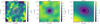 |
Fig. 1 Left: MUSTANG map, smoothed by a 9′′ FWHM kernel; middle: NIKA (2 mm) map smoothed by a 18′′ FWHM kernel; right:Bolocam map smoothed by a 58′′ FWHM kernel. Inall three panels, the red contours are those of MUSTANG, magenta contours of those of NIKA, and white contours are those of Bolocam. For MUSTANG and Bolocam, the contours start at (−)2σ, with 1σ increments. For NIKA, the contours start at (−)3σ with 2σ increments. The point source identified in Adam et al. (2015) is subtracted in the MUSTANG and NIKA maps. |
2.4 Overview of Bolocam data products
To probe a wider range of scales we complement the MUSTANG and NIKA data with SZ data from Bolocam (Glenn et al. 1998). Bolocam is a 144-element bolometer array on the Caltech Submillimeter Observatory (CSO) with a beam FWHM of 58′′ at 140 GHz and circular FOV with 8′ diameter (Glenn et al. 1998; Haig et al. 2004), which is well matched to the angular size of R500 (~ 2′) of CLJ1227. Bolocam’s conversion factor to Compton Y from μKCMB is reported as − 3.69 × 10⁻⁷, with the relativistic corrections (kBT = 12 keV) taken into account.
Bolocam was a facility instrument on the CSO from 2003 until 2012. CLJ1227 was observed with a Lissajous pattern that results in a tapered coverage dropping to 50% of the peak value at a radius of roughly 5′, and to 0 at a radius of 10′. The Bolocam maps used in this analysis are 14′ × 14′. The Bolocam data are the same as those used in Czakon et al. (2015) and Sayers et al. (2013); the details of the reduction are given therein, along with Sayers et al. (2011). The Bolocam map is shown in the right panel of Fig. 1. The reduction and calibration is similar to that used for MUSTANG, and Bolocam achieves a 5% calibration accuracy and 5′′ pointing accuracy.
2.5 Planck integrated Compton parameter
As in Adam et al. (2015), we wish to include constraints on still larger scales than reached with the aforementioned instruments, and therefore we include in this analysis the integrated Compton parameter of the cluster as measured using Planck data. We use the Planck frequency maps from 143 to 857 GHz to produce a Compton parameter map as described in Hurier et al. (2013) and Planck Collaboration XXI (2014); Planck Collaboration XXII (2016). These maps take into account known spectral dependencies and are able to mitigate non-SZ signal from the higher frequencies. The impact of the observed point source would be greatest at 353 GHz, where the flux density, extrapolated from NIKA2 bands, is significantly below the uncertainty in the Planck integrated Compton Y parameter. The resolution of this map is 7.5′, limited by the lowest frequency Planck channel map used in the reconstruction. Using this map we compute the integrated Compton parameter up to a radial distance of 15′ Uncertainties in the integrated Compton parameter are computed by integrating at random positions around the cluster. The uncertainties obtained have been also crossed-checked using Planck half-ring half difference Compton parameter map obtained as described in Planck Collaboration XXI (2014); Planck Collaboration XXII (2016). We find YCyl,(15′) = (0.94 ± 0.36) × 10−3 arcmin2.
3 Non-parametric pressure profile reconstruction via a maximum posterior distribution analysis
We perform non-parametric fits of the pressure profile of CLJ1227 on MUSTANG, NIKA, and Bolocam data maps independently. The filtering effects incurred from data processing of these instruments favors forward modeling pressure profiles and performing fits over trying to do a geometric deprojection, for example with Abel transforms (e.g., Basu et al. 2010). However, the deconvolution method employed in Basu et al. (2010) was reported to have systematic flux loss of up to 40% at R200. Our use of priors, especially of the integrated Compton parameter (Sect. 3.3) allows us to better constrain the pressure profile at larger radii. While the Abel transform and the “onion-skin” deprojection method (e.g., Kriss et al. 1983) may be computationally efficient, the calculation of errors from many deconvolved map realizations (e.g., 100 as in David et al. 2001; Basu et al. 2010) reduces the computational advantage over the approach employed in this work. Additionally, the onion-skin deprojection method typically suffers from large anti-correlations in adjacent bins and is heavily dependent on the choice of the outermost bin; these drawbacks can be significantly mitigated with regularization (e.g., Croston et al. 2006). Yet the choice of regularization parameters are non-trivial and requires cross-validation to ensure accuracy.
Before fitting the pressure profiles (Sect. 3.1), we remove a point source from the MUSTANG and NIKA maps based on previous works (Adam et al. 2015; Romero et al. 2017). Additionally, we ensure that a mean level has been removed in the MUSTANG and BOLOCAM maps. The construction of our non-parametric galaxy cluster model is described in Sect. 3.2, the fitting procedure is described in Sect. 3.3, and we review the performed validity checks in Sect. 3.4.
3.1 Preprocessing
A point source at 4.6σ significance (~0.5 mJy) in MUSTANG was reported in Korngut et al. (2011), but is not evident in the MUSTANG data as reprocessed in Romero et al. (2017). A short VLA filler observation (VLA-12A-340, D-array, at 7 GHz) was performed to follow up this potential source (at RA 12:26:58.0 and Dec +33:32:59), but to a limit of ~ 50 μJy nothing is seen (Romero et al. 2017). At 500 μm, Herschel-SPIRE has a point source sensitivity of ~8 Jy, but no point source is evident at the above location.
Adam et al. (2015) find a point source at a different location, RA 12:26:59.855 and Dec +33:32:35.21, with a flux density of 6.8 ± 0.7 (stat.) ± 1.0 (cal.) mJy at 260 GHz and 1.9 ± 0.2 (stat.) at 150 GHz. For this source, at 500 μm, Herschel-SPIRE finds a flux of 100 ± 8 mJy 2. A point source at this location is fit to the MUSTANG data with a flux density of 0.36 ± 0.11 mJy (Romero et al. 2017). We subtract this point source from the NIKA and MUSTANG maps using the above flux density values. In the Bolocam data, the point source is faint enough to not be a concern, given Bolocam’s beam size.
We also wish to account for any mean level before fitting our cluster model, especially because there is a degeneracy between the mean level and the cluster model, and the mean level can typically be well constrained a priori. The mean level in the MUSTANG map is calculated as the mean within the inner arcminute MUSTANG noise map, which was created from time-flipped time-ordered data. We subtract the mean level from the MUSTANG map before fitting a cluster model. Within NIKA data, a mean level is calculated within the timestreams for data falling outside the masked region. This mean level is subtracted within the timestream processing of NIKA data. The Bolocam map already has a mean level subtracted.
3.2 Non-parametric pressure profile models
Our non-parametric pressure profile reconstruction assumes spherical symmetry and power law interpolation between radial bins. Because we employ analytic integrals, we can integrate from zero to a finite radius, and from a finite radius to infinity, with some clear restrictions on the power laws when doing so. The analytic integration has been employed before (e.g., Vikhlinin et al. 2001; Korngut et al. 2011; Sarazin et al. 2016). Here, we resolve previous limitations (Appendix A) found with certain power laws for which the previously given analytic formulation are undefined (Korngut et al. 2011; Sarazin et al. 2016), but which are necessary to be covered in our analysis. Our fitting algorithm is applied to each dataset independently; therefore, cluster models are binned and gridded differently for each dataset. Radial bins are defined so that each bin is at least as wide as a beam width (FWHM), with the additional constraint that the outer most bin is beyond the FOV of the instrument.
For eachbin, i, we denote the radius as Ri, and assign a pressure Pi. The interpolation of pressure between at a radius r, Ri < r < Ri+1 is given by  , where α is calculated as:
 (1) For radii interior to our innermost radial bin (R1), we extrapolate using the same power law as between R1 and R2. Similarly, for radii exterior to our outermost radial bin (Rn), we extrapolate using the same power law as between Rn−1 and Rn. We therefore put a prior on our outermost slope such that α > 1, and the integrated quantity is finite.
We note that for a non-rotating, spherical object in hydrostatic equilibrium (HSE) under entirely thermal pressure support, the power law should be limited to α > 4 in order to avoid having infinite mass (see Appendix B). While we recognize this limit here, during fitting we only enforce α > 1.
Given the restrictions of ellipsoidal symmetry and a power law dependence of the integrated quantity (pressure) on the ellipsoidal radius, it is possible to calculate the integral along the line of sight analytically (e.g., Vikhlinin et al. 2001; Korngut et al. 2011). We follow principally the formulation provided in Korngut et al. (2011). As noted in Sarazin et al. (2016), there are certain power laws (α∕2 = p = 1∕2, 0, −1∕2, −1, −3∕2, ...) for which the formulation given in Korngut et al. (2011) fails, but a reformulation provides a valid integration. More generally, the formulation fails for α∕2 = p < −1∕2. While a negative index indicates a rise in pressure with radius (atypical), this could arise, especially localized, from shocks, for example. We also wish to minimize our restrictions on the power laws (between bins) so as to minimize induced correlations between bins. Therefore, we implement extensions to the canonical formulation that allow us to integrate within finite regions (spheres or shells that extend only to a finite radius). These extensions and reformulations of specific half integers are described in Appendix A.
The profiles, integrated along the line of sight (ℓ) are calculated as the Compton Y parameter:
 (2) are converted into the units of the original data map. Maps are gridded by assuming a linear interpolation of the 1D (radial) profiles. When gridding our bulk ICM component, we adopt the ACCEPT centroid of CLJ1227, and grid a larger map than used for fitting. These (2D) maps are then convolved with the respective beam and transfer function. Aliasing is alleviated by trimming the region not fitted. For MUSTANG, NIKA, and Bolocam, we fit a square region about the centroid with lengths of 2′, 4′, and 13.33′ respectively.
3.3 Fitting Algorithm
We employ a maximum posterior distribution algorithm, and take our noise to be Gaussian. In previous works, NIKA and MUSTANG noise have been taken as uncorrelated (e.g., Romero et al. 2015, 2017; Adam et al. 2015). Bolocam noise has been taken as approximately uncorrelated, but 1000 noise realizations, which included CMB and point source estimates, are provided to allow for a more accurate noise estimation (Sayers et al. 2011). We calculate the two-dimensional power spectrum for noise maps of each dataset. On the scales we use to constrain the models, the noise is consistent with white noise.
We calculate the final probability of our models by applying priors as prescribed by Bayes’ Theorem. On each of the pressure bins, we assign strict priors that Pi > 0, and as previously mentioned, the last bin has a prior that on its associated power law slope: α > 1. We allow for the choice of including a Gaussian prior on the integrated Compton Y parameter:
 (3) where the integral over solid angle taken within a given radius is generally referred to as the cylindrical Compton Y value (Ycyl). We calculate Ycyl using the un-filtered Compton y profile (before convolution with an instrument’s beam and transfer function). The prior on Y comes from Planck data (Planck Collaboration XXIX 2014) as discussed in Sect. 2.5. In particular, we take the prior Ycyl(15′) = (0.94 ± 0.36) × 10−3 arcmin2.
We employ the described probability function in a python Markov chain Monte Carlo (MCMC) package, emcee (Foreman-Mackey et al. 2013). It provides fairly accessible implementation and parallelized sampling.
3.4 Validation and performance of fitting algorithm
Our algorithm is first tested with mock cluster observations. We create mock observations by adding a noise realization (created from jack-knifed timestreams) for each of the three maps to the corresponding filtered map of a previously determined (Romero et al. 2017) gNFW profile. We perform initial tests to validate the number of bins chosen. The resolution (FWHM) and FOV of our instruments (see Sect. 3.2) suggest that between four and eight bins are appropriate. We cover this range, with fits run withfour, six, and eight bins with two model constructions. The first, as described in Sect. 3.2, and a second being uniform spherical pressure bins. F-tests on the posterior distributions do not indicate a preference in the number of bins used. We consider how well the recovered pressure profile matches the input gNFW pressure profile. To do so, we calculate χ2 of the fitted pressure profile relative to the input gNFW and find that the reduced χ2 is minimized when using six bins for MUSTANG and Bolocam. For NIKA, it is minimized at eight bins, but this is likely influenced by the prior on the integrated Compton Y, which is only implemented on the NIKA data. A difference of χ2 test results in p-values for preferring eight bins over six bins for MUSTANG, NIKA, and Bolocam are 0.015, 0.80, and 0.50. Except for MUSTANG, it appears that statistically there is not a significant preference. Given satisfactory fits with six bins for all instruments, and a preference from MUSTANG, we adopt six bins across the board.
We further test the dependence of the fit results on initial guess of the pressure values, and find that this dependence is minimal. We change the input guesses by the following factors fP = [0.01, 0.1, 0.33, 3.0, 10, 100], and perform the fits on the mock cluster observations. We find that at worst, we see that the results are generally within 7% of each other, with the exception that the outermost bin may see a dispersion up to 20%, and one of the inner bins in NIKA data sees a dispersion of 14%. However, if we limit the span to just fP = [0.1, 0.33, 3.0, 10], the dispersions are less than 6% for all but the outer bins, which see dispersions less than 10%.
Finally, across the above suite of tests (number of bins, uniform or power law distribution within a bin, and initial guesses), we find that the outermost bins in MUSTANG and Bolocam are biased high, where for Bolocam, the second most outer bin is also biased high. We find that in the production of the models, this appears to arise with the application of the transfer functions of these instruments. In particular, with Bolocam, the transfer function produces artifacts at large radii (r≳1000 kpc). As we define the outermost bin of our power law model to extend to infinity, truncating, or reducing the number of bins does not resolve this bias. Rather, we find it best to retain the bins in the map fitting procedure and to trim them in subsequent analyses. Therefore, in our analysis of real data, six bins are used within the fitting procedure, and we retain five, six, and four bins for MUSTANG, NIKA, and Bolocam respectively for subsequent analysis and discussion.
We show the fits to our mock observations with this six-bin, power-law model in Fig. 2, and note that the reconstructed profiles are consistent with the input profile. Our input gNFW model has been taken from Romero et al. (2017), and our output model is fit as prescribed in Sect. 5.
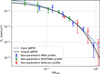 |
Fig. 2 Non-parametric pressure profiles as determined via each mock observation individually, and the gNFW (parametric) pressure profile as simultaneously fit to the non-parametric pressure profiles. The error bars are statistical, from the MCMC fits. |
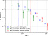 |
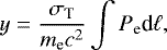
Fig. 3 Non-parametric pressure profiles as determined via each dataset individually. The error bars are statistical, from the MCMC fits. The vertical dashed and dotted lines correspond to the half width at half maximum (HWHM) and FOV/2 (i.e.,radial FOV), respectively. |
4 Non-parametric pressure profile results
As noted in the previous section, we trim the outer one and two bins in MUSTANG and Bolocam respectively from subsequent analysis. Wetrim these bins due to bias in the fits on simulated data. The results, shown in Fig. 3 are also tabulated in Table 2 with trimmed points in red.
From the Monte Carlo chains of the non-parametric fits, we determine the covariance matrix of the pressure bins for each dataset as:
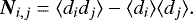 (4) This formulation assumes that the data is well described by a Gaussian distribution; however Table 2 shows that the distributions of binned pressures are asymmetric. From the residuals in Fig. 6, which account for the asymmetries, we find that assuming Gaussian distributions does not adversely impact our results, particularly as we have employed the covariance matrix in this work.
We show the correlation matrices in Fig. 4. We notice that any two adjacent bins are negatively correlated, and by extension, bins spaced two apart (e.g., bins one and three) are positively correlated. The maximum amplitude of off-diagonal correlations is 0.13, 0.05, and 0.05 for MUSTANG, NIKA, and Bolocam respectively. These are relatively small correlations,especially when contrasted with Sayers et al. (2013), whose correlations (with 13 radial bins) appears to be over 0.5 for the someadjacent radial bins.
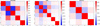 |
Fig. 4 Non-parametric bin correlation matrices. Left: MUSTANG. Middle: NIKA. Right: Bolocam. The coloring is scaled to make the magnitude of off-diagonal terms more apparent, and the range changes for each instrument. |
Non parametric pressure profile fits.
5 Parametric pressure profile (gNFW) fits
We wish to compare our non-parametric fits to each other (testing consistency between instruments) and to previous results of cluster pressure profiles. We note that at a z = 0.89, CLJ1227 is at a high redshift, and although only being one cluster, serves as an initial test of the universality of so-called universal pressure profile (Arnaud et al. 2010), which was derived from a local (z < 0.2) sample of clusters. Given the prevalence of parametric pressure profiles in previous analyses, and in particular, the gNFW parameterization, we fit a gNFW profile to our non-parametric pressure profile constraints. The gNFW profile is given as:
![Mathematical equation: \begin{equation*} \tilde{P} = \frac{P_0}{(C_{500} X)^{\gamma} [1 + (C_{500} X)^{\alpha}]^{(\beta - \gamma)/\alpha}}\end{equation*}](/articles/aa/full_html/2018/04/aa31599-17/aa31599-17-eq6.png) (5)
(5)
where X = R∕R500, and C500 is the concentration parameter; one can also write (C500X) as (R∕Rp), where Rp = R500∕C500. The exponentials α, β, and γ are commonly cited as the (logarithmic) slopes at moderate, large, and small radii. However, α should be understood to govern the rate of turnover between the two slopes, β and γ.
We aim to constrain all parameters within the gNFW profile, but find that α is driven to high values, and furthermore the constraints are very poor for these high values. Therefore, we choose to restrict α to 1.05, the value found in A10. We further include nuisance parameters of calibration offsets for each dataset. The calibration uncertainties for NIKA, MUSTANG, and Bolocam are taken to be 7%, 10%, and 5% respectively. The mean level in each dataset has already been removed or fitted, so it is not considered here. We use the full covariance matrices from our non-parametric fits.
We find gNFW parameters of [P0, C500, β, and γ] = [ ,
,  ,
, , and
, and  ]. We take our best-fit value as the 50th percentile in each marginalized parameter distribution. The error bars are calculated at the corresponding 1σ (50 ± 34%) percentiles. The power law slope γ is within the typical value range found in previous gNFW constraints (e.g., Nagai et al. 2007; Arnaud et al. 2010; Sayers et al. 2013), on CLJ1227 as well as general cluster samples. However, our value of β is less than expected; moreover, for a non-rotating spherical cluster in HSE under thermal pressure support β ≤4 would indicate an unbounded mass at arbitrarily large radii (Appendix B). Similarly, P0 and C500 are larger than generally found. Given the degeneracy between β, P0, and C500, as shown inFig. 5, and shape of the pressure profile, these atypical values of β and P0 appear to be driven by C500 being pushed to larger values, where a large C500 value indicates that the scale radius (transition in pressure profile slopes) occurs at a relatively small radius.
We also note that the value of C500 itself may not be nearly as high if a smaller value of R500 is adopted (implying a smaller M500 and P500.) This may well be the case, as several other studies conclude that R500 < 1000 kpc (e.g., Rumsey et al. 2016; Mroczkowski et al. 2009).
Setting aside the variations in parameter values themselves, we see in Fig. 6 that our gNFW fit is in agreement for R≳0.3 R500. In the central regions, our fit shows greater pressure than would be inferred from A10 or Planck Collaboration V (2013), but is consistent with Romero et al. (2017).
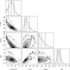 |
Fig. 5 Parameter constraints for our gNFW model: P0, rp, γ, and β. Recall that C500 = R500∕Rp. The dashed lines on the individual parameter histograms show 14th, 50th, and 86th percentiles. The contour plots of two parameters have 1σ, 2σ, and 3σ contours. |
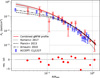 |
Fig. 6 OurgNFW (parametric) pressure profile as simultaneously fit to the non-parametric pressure profiles is shown in red. The error bars are statistical, from the MCMC fits. The residual significances (σ, lower panel) are calculated from the asymmetric statistical errors (Table 2) and calibration errors. The non-parametric symbol-to-instrument association remains the same as in Figs. 2 and 3. The MUSTANG point that falls well (~ − 2.8σ) below the gNFW pressure profile (close to 0.1 R500) is of note and discussed in Sect. 6. The last two NIKA points fall − 5.5σ and − 2.8σ below the gNFW profile. |
6 Discussion
Our non-parametric fits are well reproduced with varying input parameters (Sect. 3.4). This procedure can be readily applied to ellipsoidal cluster geometries, and could also be modified to include shock components. Given the potential for ellipsoidal clusters and presence of shocks, we find that the ability to analyze both the global and local electron pressure in clusters within a non-parametric approach will be of considerable utility as sensitive, high-resolution, SZ observations of individual clusters become more commonplace, especially at high redshift.
While our estimation of outer pressure bins may be influenced by the mean level in a map, or a poorly constrained transfer function, we see that the inner bins remain largely unaffected (Sect. 3.4). We find good agreement in our non-parametric fits between MUSTANG, NIKA, and Bolocam, as all but two points lie within 2.5σ of the fitted gNFW profile. The inner point that falls below the gNFW profile comes from MUSTANG fits, and is only ~ 2σ discrepant from the gNFW profile.
This deviation (at a radius of ~12′′ or 0.1 R500) is consistent with the location of the point source found in Korngut et al. (2011), and performing a fit on mock observations, where we add a 0.5 mJy source (at 90 GHz) at this location, can reproduce the observed deviation. Within the NIKA (150 GHz) data, no evidence for a weak point source is seen, although, we note that simulated observations of a 1.4 mJy source at the same radial distance does not have a significant effect on the non-parametric fits, relative to the fits of the simulated observations without a point source. At other wavelengths, in the 260 GHz NIKA data (Adam et al. 2015), as well as at lower frequencies and higher frequencies (Sect. 3.1), no evidence is seen for a point source.
Within our gNFW fits, if α is left unconstrained, we find that large values of α are preferred, indicating a rapid transition between the inner and outer pressure profile slopes. Thisturnover is largely driven by NIKA, where, in Fig. 6 (with α fixed), the outer two points fall − 5.5σ and − 2.8σ away from the fitted gNFW pressure profile. NIKA has the best coverage in the spatial region where this transition occurs, and additionally,NIKA has the strongest detection of the cluster and places the greatest constraints on the pressure profile, globally.
Our gNFW pressure profile fit shows a higher core pressure than that of other sample-averaged gNFW profiles (see Fig. 6). Many sample-averaged profile studies have subdivided their samples by dynamical state and find that cool-core clusters tend to have steeper inner pressure profiles (e.g., Arnaud et al. 2010; Planck Collaboration V 2013; Sayers et al. 2013; Romero et al. 2017), and therefore one might infer that CLJ1227 is also a core core cluster. However, X-ray data show that the core is relatively hot (13 keV; Maughan et al. 2007), thus highlighting that dynamical state is certainly not well established via a pressure profile alone.
We compare our parametric and non-parametric profiles to non-parametric profiles derived in ACCEPT (Cavagnolo et al. 2009), a publicly available database of data products from Chandra observations of galaxy clusters3. We find agreement with the ACCEPT profile (Fig. 6), noting that both the ACCEPT and our pressure profiles rise above the ensemble averages of (Planck Collaboration V (2013; z < 0.5) and A10 (z < 0.2. In an X-raystudy of 80 South Pole Telescope (SPT) selected clusters, McDonald et al. (2014) found lower central pressure, relative to the universal pressure profile in A10, for their subsample of high-(z > 0.6) redshift clusters. Where CLJ1227 is at z = 0.89, its increased central pressure relative to A10 is counter to the trend in McDonald et al. (2014), is suggestive that CLJ1227 is somehow unique. Indeed, CLJ1227 is among the most massive clusters at z > 0.6 (e.g., Menanteau et al. 2012).
The uniqueness of CLJ1227 is likely enhanced given the various studies supporting merger activity. Maughan et al. (2007) interpreted the hot ICM to be suggestive of a merger event. This interpretation is echoed in Jee & Tyson (2009), whose lensing analysis supports a picture in which the dark matter distribution appears undisturbed on large scales, but shows a clear bimodality in the central region, and conclude by postulating an early-stage head-on merger scenario. Rumsey et al. (2016) support the early stage merger scenario primarily from the differences seen in scaling quantities (YX) between X-ray and SZ (AMI) data.
The profiles recovered here are consistent with the parametric profiles found in Adam et al. (2015). We note that the transition in the pressure profile from the inner to outer profile appears gradual in Adam et al. (2015), whereas our work is suggestive of a sharper transition, especially when we allow α to vary (Sect. 5). In none of the SZ maps used in this analysis is there clear (significant) substructure which may be inferred to cause elevated pressure. Where a merger in the plane of the sky may produce observable shocks, especially via high-resolution SZ observations, we find the lack of substructure in our study to be consistent with a head-on merger. Given the noise levels achieved by NIKA and MUSTANG, if substructure exists in the core, it may require yet higher resolution to observe it.
This merger scenario could still be consistent with our findings, as a merger affecting the central pressure should indeed increase the pressure there. Provided that the system is not in equilibrium, and in particular, that increased gas pressure has not propagated to the outer extent of the cluster, then this scenario would be consistent with the cluster pressure profiles that we have reconstructed (both the non-parametric and subsequent parametric profiles). An approach of determining non-parametric profiles, such as that presented here, will be useful for a more accurate analysis of pressure fluctuations and will inform the degree of non-thermal pressure support (e.g., Khatri & Gaspari 2016).
7 Conclusions
We developed an algorithm to determine a non-parametric pressure profile for galaxy clusters. This method is of particular utility to SZ observations, where the filtering effects from data processing favor fitting forward modeled pressure profiles, as opposed to deriving non-parametric pressure profiles via geometric deprojection. Our fitting algorithm is robust with respect to input parameters, bin spacing, and instrumental setup specifics. While the constraints of single-dish SZ observations beyond the FOV for a given instrument are poor, we find that the inclusion of such a bin appears to improve the robustness of the pressure constraints within the FOV.
We have applied this algorithm to SZ observations of the high redshift cluster (z = 0.89) CLJ1227 from MUSTANG, NIKA, and Bolocam. In doing so, we cover a radial range 0.05 R500 < r < 1.1 R500, continuously recovering spatial scales in this range, and find consistency among the non-parametric fits of the individual instruments. Furthermore, parametric best fits indicate a gNFW profile with a relatively small scale radius (rp; rp = C500∕R500). If left unconstrained, α tends toward largevalues, indicating a rapid transition at this scale radius between the inner and outer slope. This rapid transition is consistent across all three instruments, where NIKA is most sensitive to this transition region and indeed NIKA data alone favors a rapid transition. This rapid transition is also supported by MUSTANG data, in part due to the drop in recovered pressure at a radius, 9′′ < r < 23′′ (0.07 R500 < r < 0.18 R500).
Empirical investigations into potential point source contamination within this region (9′′ < r < 23′′) indicate thatsuch a point source would have to be ~0.5 mJy at 90 GHz. However, the lack of support for such a point source at other wavelengths leads us to doubt this potential explanation for the dip in MUSTANG pressure between 9′′ < r < 23′′.
Our non-parametric fits of the pressure profile of CLJ1227 are consistent with a smooth (parameterized) pressure profile. Yet, we have the advantage that deviations from a parameterized pressure profile will be more evident, localized, and allow for easier investigation of potential contamination or deviations from hydrostatic equilibrium. In its current implementation, this approach is relatively intuitive, robust, and fast (due to the analytic integration). While a spherical cluster was assumed for this analysis, the approach already allows for an ellipsoidal geometry. We also foresee the potential to extend this approach to include analysis of slices within an ellipse, which will prove useful for investigating shocks. We anticipate that this versatility will be useful in analysis of the NIKA2 SZ large program Comis et al. (2016) and other future SZ observations.
Acknowledgements
The National Radio Astronomy Observatory is a facility of the National Science Foundation which is operated under cooperative agreement with Associated Universities, Inc. MUSTANG data was retrieved from https://safe.nrao.edu/wiki/bin/view/GB/Pennarray/MUSTANG_CLASH. Original MUSTANG data was taken under NRAO proposal IDs GBT/09A-052, GBT/09C-059. NIKA data of CLJ1227 can be found at http://vizier.cfa.harvard.edu/viz-bin/VizieR?-source=J/A+A/576/A12. Bolocam data was retrieved from http://irsa.ipac.caltech.edu/data/Planck/release_2/ancillary-data/bolocam/. The Bolocam observations presented here were obtained from the Caltech Submillimeter Observatory, which, when the data used in this analysis were taken, was operated by the California Institute of Technology under cooperative agreement with the National Science Foundation. Bolocam was constructed and commissioned using funds from NSF/AST-9618798, NSF/AST-0098737, NSF/AST-9980846, NSF/AST-0229008, and NSF/AST-0206158. Bolocam observations were partially supported by the Gordon and Betty Moore Foundation, the Jet Propulsion Laboratory Research and Technology Development Program, as well as the National Science Council of Taiwan grant NSC100-2112-M-001-008-MY3. We would like to thank the IRAM staff for their support during the NIKA campaigns. The NIKA dilution cryostat has been designed and built at the Institut Néel. In particular, we acknowledge the crucial contribution of the Cryogenics Group, and in particular Gregory Garde, Henri Rodenas, Jean-Paul Leggeri, Philippe Camus. This work has been partially funded by the Foundation Nanoscience Grenoble, the LabEx FOCUS ANR-11-LABX-0013 and the ANR under the contracts MKIDS, NIKA and ANR-15-CE31-0017. This work has benefited from the support of the European Research Council Advanced Grant ORISTARS under the European Union’s Seventh Framework Programme (Grant Agreement No. 291294). We acknowledge fundings from the ENIGMASS French LabEx (R.A. and F.R.), the CNES post-doctoral fellowship program (R.A.), the CNES doctoral fellowship program (A.R.) and the FOCUS French LabEx doctoral fellowship program (A.R.). The authors would like to thank the anonymous referee for helpful comments on this manuscript.
Appendix A Analytic integrals of ellipsoidally symmetric power laws
In our non-parametric pressure bin analysis, we assume that the pressure distribution is spherically symmetric. As the formalism is applicable to ellipsoidally symmetric systems, we present the formulations in ellipsoidal generality, with the condition that an axis (taken as the z axis) is along theline of sight. Our quantity to be integrated along the line of sight is denoted as ϵ, and has the following behavior:
 (A.1)
(A.1)
where ϵi is a normalization for the pressure within bin i; ai, bi, and ci are the ellipsoidal scalings of their respective axes, with the z-axis being along the line of sight, and − 2Qi is the slopeof the pressure profile. We define an ellipsoidal radius, 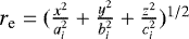 . A pressure bin can be in one of three cases: (C1) an ellipsoid of finite extent; (C2) a shell of finite extent; and (C3) a shell of infinite extent. We use these markers (C1, C2, and C3) as superscripts when writing definitions per case. The pressure distribution can be rewritten as follows:
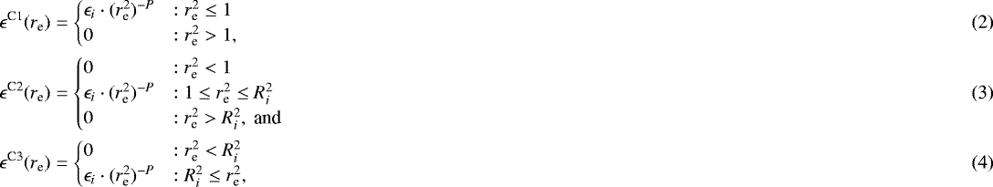 (A.2) (A.3) (A.4)
where Ri is a boundary radius (the outer boundary in Case 2). Given a cluster profile with more than three bins, we end up with many bins in Case 2, in which case we rescale ai, bi, ci, and subsequently Ri each time to properly normalize each bin (ϵi)
Let us define
 (A.5)
(A.5)
where  . While the integration of each bin will share this expression, the actual values may change depending on ai, bi, and ci used for each bin (as above, when multiple bins fall into Case 2). We write the integration of ϵ(re) along the line of sight as:
 (A.6)
(A.6)
where z0 is the outer limit (in z) of the region in question. Over the three cases, the solutions are as follows:
 (A.7) (A.8) (A.9)
Here,  , or
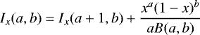
, or  is the incomplete beta function, often denoted as Ix(a, b). For the discussion of the gamma and incomplete beta function (below), x, y, a, and b serve as dummy variables. Given our use of the gamma and incomplete beta functions, it is important to recognize their limitations. Specifically, Γ(a) is undefined for
  (negative integers, including zero). The incomplete beta function, having a = Qi − 0.5 and b = 0.5 suffers from undefined values for
  as well as
  . Finally, all incomplete beta functions are generally defined for B(a, b) that Re(a) > 0 and Re(b) > 0. However, the relation of the incomplete beta function (Ix):
 (A.10)
allows us to extend the function into the negative domain (for a, which we take as Qi − 0.5).
To deal with the limitation, generally seen as:  , we derive another approach. From Eq. (A.6), we can substitute variables (t = z∕(cA)) to arrive at:
 (A.11) (A.12) (A.13)
This must then be extended, and is done so with the relation:
 (A.14)
Given the values of interest/applicability ( ), this extension is perfectly applicable, and we will end in well-behaved functions; either:
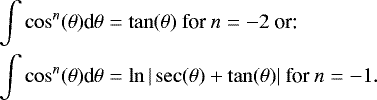
The only case where this analytic integration fails is for Qi < 0.5 when integrating out to infinity, which is fine, as this must diverge in any case.
Appendix B Requirements for finite mass for a non-rotating, spherical object under HSE
For a non-rotating, spherical object in hydrostatic equilibrium (HSE) under thermal pressure support, we have:
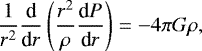 (B.1)
(B.1)
where G is the Newtonian constant of gravity and ρ is the (total) matter density (Landau & Lifshitz 1959). Moreover, we can integrate the first derivative and find:
 (B.2)
(B.2)
where we have used the integral
 (B.3)
(B.3)
and note that under this formulation ρ must have a dependence of r−δ, where δ > 3 to have a finite mass at an arbitrarily large radius. Therefore, returning to Eq. (B.2), we find that M(r) can be written as:
 (B.4)
(B.4)
where P0 and ρ0 are simply normalizations of the pressure and density respectively. The mass under hydrostatic equilibrium will then have the radial dependence as r1+δ−α, where again, δ > 3. Therefore, we find that α ≥ 4 is required for a finite mass of an object, under the assumptions stated above.
References
- Adam, R., Comis, B., Macías-Pérez, J. F., et al. 2014, A&A, 569, A66 [NASA ADS] [CrossRef] [EDP Sciences] [Google Scholar]
- Adam, R., Comis, B., Macías-Pérez, J.-F., et al. 2015, A&A, 576, A12 [NASA ADS] [CrossRef] [EDP Sciences] [Google Scholar]
- Adam, R., Comis, B., Bartalucci, I., et al. 2016, A&A, 586, A122 [NASA ADS] [CrossRef] [EDP Sciences] [Google Scholar]
- Arnaud, M., Pratt, G. W., Piffaretti, R., et al. 2010, A&A, 517, A92 [NASA ADS] [CrossRef] [EDP Sciences] [Google Scholar]
- Basu, K., Zhang, Y.-Y., Sommer, M. W., et al. 2010, A&A, 519, A29 [NASA ADS] [CrossRef] [EDP Sciences] [Google Scholar]
- Battaglia, N., Bond, J. R., Pfrommer, C., & Sievers, J. L. 2012, ApJ, 758, 75 [NASA ADS] [CrossRef] [Google Scholar]
- Bonamente, M., Joy, M. K., LaRoque, S. J., et al. 2006, ApJ, 647, 25 [NASA ADS] [CrossRef] [Google Scholar]
- Bonamente, M., Hasler, N., Bulbul, E., et al. 2012, New J. Phys., 14, 025010 [NASA ADS] [CrossRef] [Google Scholar]
- Borgani, S., Murante, G., Springel, V., et al. 2004, MNRAS, 348, 1078 [NASA ADS] [CrossRef] [Google Scholar]
- Bulbul, G. E., Hasler, N., Bonamente, M., & Joy, M. 2010, ApJ, 720, 1038 [NASA ADS] [CrossRef] [Google Scholar]
- Calvo, M., Benoît, A., Catalano, A., et al. 2016, J. Low Temp. Phys., 184, 816 [NASA ADS] [CrossRef] [Google Scholar]
- Catalano, A., Calvo, M., Ponthieu, N., et al. 2014, A&A, 569, A9 [NASA ADS] [CrossRef] [EDP Sciences] [Google Scholar]
- Cavagnolo, K. W., Donahue, M., Voit, G. M., & Sun, M. 2009, ApJS, 182, 12 [NASA ADS] [CrossRef] [Google Scholar]
- Cavaliere, A., & Fusco-Femiano, R. 1978, A&A, 70, 677 [NASA ADS] [Google Scholar]
- Comis, B., Adam, R., Ade, P., et al. 2016, ArXiv e-prints [arXiv:1605.09549] [Google Scholar]
- Croston, J. H., Arnaud, M., Pointecouteau, E., & Pratt, G. W. 2006, A&A, 459, 1007 [NASA ADS] [CrossRef] [EDP Sciences] [Google Scholar]
- Czakon, N. G., Sayers, J., Mantz, A., et al. 2015, ApJ, 806, 18 [NASA ADS] [CrossRef] [Google Scholar]
- David, L. P., Nulsen, P. E. J., McNamara, B. R., et al. 2001, ApJ, 557, 546 [NASA ADS] [CrossRef] [Google Scholar]
- de Haan, T., Benson, B. A., Bleem, L. E., et al. 2016, ApJ, 832, 95 [NASA ADS] [CrossRef] [Google Scholar]
- Dicker, S. R., Korngut, P. M., Mason, B. S., et al. 2008, in SPIE Conf. Ser., 7020, 702005 [Google Scholar]
- Dicker, S. R., Ade, P. A. R., Aguirre, J., et al. 2014, in SPIE Conf. Ser., 9153, 0 [Google Scholar]
- Ebeling, H., Edge, A. C., & Henry, J. P. 2001, ApJ, 553, 668 [Google Scholar]
- Foreman-Mackey, D., Hogg, D. W., Lang, D., & Goodman, J. 2013, PASP, 125, 306 [CrossRef] [Google Scholar]
- Glenn, J., Bock, J. J., Chattopadhyay, G., et al. 1998, Proc. SPIE, 3357, 326 [NASA ADS] [CrossRef] [Google Scholar]
- Haig, D. J., Ade, P. A. R., Aguirre, J. E., et al. 2004, in SPIE Conf. Ser. 5498, eds. C. M. Bradford, P. A. R. Ade, J. E. Aguirre, et al., 78 [Google Scholar]
- Hasselfield, M., Hilton, M., Marriage, T. A., et al. 2013, J. Cosmol. Astropart. Phys., 7, 8 [Google Scholar]
- Hurier, G., Macías-Pérez, J. F., & Hildebrandt, S. 2013, A&A, 558, A118 [NASA ADS] [CrossRef] [EDP Sciences] [Google Scholar]
- Itoh, N., Kohyama, Y., & Nozawa, S. 1998, ApJ, 502, 7 [NASA ADS] [CrossRef] [Google Scholar]
- Jee, M. J., & Tyson, J. A. 2009, ApJ, 691, 1337 [NASA ADS] [CrossRef] [Google Scholar]
- Jewell, P. R., & Prestage, R. M. 2004, in Ground-based Telescopes, ed. J. M. Oschmann, Jr., SPIE Conf. Ser., 5489, 312 [NASA ADS] [Google Scholar]
- Joy, M., LaRoque, S., Grego, L., et al. 2001, ApJ, 551, L1 [NASA ADS] [CrossRef] [Google Scholar]
- Kaiser, N. 1986, MNRAS, 222, 323 [NASA ADS] [CrossRef] [Google Scholar]
- Khatri, R., & Gaspari, M. 2016, MNRAS, 463, 655 [NASA ADS] [CrossRef] [Google Scholar]
- Kitayama, T., Ueda, S., Takakuwa, S., et al. 2016, PASJ, 68, 88 [NASA ADS] [CrossRef] [Google Scholar]
- Korngut, P. M., Dicker, S. R., Reese, E. D., et al. 2011, ApJ, 734, 10 [NASA ADS] [CrossRef] [Google Scholar]
- Kravtsov, A. V., & Borgani, S. 2012, ARA&A, 50, 353 [NASA ADS] [CrossRef] [Google Scholar]
- Kriss, G. A., Cioffi, D. F., & Canizares, C. R. 1983, ApJ, 272, 439 [NASA ADS] [CrossRef] [Google Scholar]
- Landau, L. D., & Lifshitz, E. M. 1959, Fluid mechanics (Oxford: Pergamon Press) [Google Scholar]
- Mantz, A., Allen, S. W., Ebeling, H., Rapetti, D., & Drlica-Wagner, A. 2010, MNRAS, 406, 1773 [NASA ADS] [Google Scholar]
- Mason, B. S., Dicker, S. R., Korngut, P. M., et al. 2010, ApJ, 716, 739 [NASA ADS] [CrossRef] [Google Scholar]
- Maughan, B. J., Jones, L. R., Ebeling, H., & Scharf, C. 2004, MNRAS, 351, 1193 [NASA ADS] [CrossRef] [Google Scholar]
- Maughan, B. J., Jones, C., Jones, L. R., & Van Speybroeck L. 2007, ApJ, 659, 1125 [NASA ADS] [CrossRef] [Google Scholar]
- McDonald, M., Benson, B. A., Vikhlinin, A., et al. 2014, ApJ, 794, 67 [NASA ADS] [CrossRef] [Google Scholar]
- Menanteau, F., Hughes, J. P., Sifón, C., et al. 2012, ApJ, 748, 7 [NASA ADS] [CrossRef] [Google Scholar]
- Monfardini, A., Swenson, L. J., Bideaud, A., et al. 2010, A&A, 521, A29 [NASA ADS] [CrossRef] [EDP Sciences] [Google Scholar]
- Monfardini, A., Adam, R., Adane, A., et al. 2014, J. Low Temp. Phys., 176, 787 [NASA ADS] [CrossRef] [Google Scholar]
- Mroczkowski, T. 2011, ApJ, 728, L35 [NASA ADS] [CrossRef] [Google Scholar]
- Mroczkowski, T., Bonamente, M., Carlstrom, J. E., et al. 2009, ApJ, 694, 1034 [NASA ADS] [CrossRef] [Google Scholar]
- Muchovej, S., Mroczkowski, T., Carlstrom, J. E., et al. 2007, ApJ, 663, 708 [NASA ADS] [CrossRef] [Google Scholar]
- Nagai, D., Kravtsov, A. V., & Vikhlinin, A. 2007, ApJ, 668, 1 [NASA ADS] [CrossRef] [Google Scholar]
- Planck Collaboration V 2013, A&A, 558, C2 [CrossRef] [EDP Sciences] [Google Scholar]
- Planck Collaboration XXI 2014, A&A, 571, A21 [NASA ADS] [CrossRef] [EDP Sciences] [Google Scholar]
- Planck Collaboration XXIX 2014, A&A, 571, A29 [NASA ADS] [CrossRef] [EDP Sciences] [Google Scholar]
- Planck Collaboration XIII 2016, A&A, 594, A13 [NASA ADS] [CrossRef] [EDP Sciences] [Google Scholar]
- Planck Collaboration XXII 2016, A&A, 594, A22 [NASA ADS] [CrossRef] [EDP Sciences] [Google Scholar]
- Planck Collaboration XXIV 2016, A&A, 594, A24 [NASA ADS] [CrossRef] [EDP Sciences] [Google Scholar]
- Press, W. H., & Schechter, P. 1974, ApJ, 187, 425 [NASA ADS] [CrossRef] [Google Scholar]
- Romero, C. E., Mason, B. S., Sayers, J., et al. 2015, ApJ, 807, 121 [NASA ADS] [CrossRef] [Google Scholar]
- Romero, C. E., Mason, B. S., Sayers, J., et al. 2017, ApJ, 838, 86 [NASA ADS] [CrossRef] [Google Scholar]
- Rumsey, C., Olamaie, M., Perrott, Y. C., et al. 2016, MNRAS, 460, 569 [NASA ADS] [CrossRef] [Google Scholar]
- Ruppin, F., Adam, R., Comis, B., et al. 2017, A&A, 597, A110 [NASA ADS] [CrossRef] [EDP Sciences] [Google Scholar]
- Sarazin, C. L., Finoguenov, A., Wik, D. R., & Clarke, T. E. 2016, ApJ, submitted [arxiv:1606.07433] [Google Scholar]
- Sayers, J., Golwala, S. R., Ameglio, S., & Pierpaoli, E. 2011, ApJ, 728, 39 [NASA ADS] [CrossRef] [Google Scholar]
- Sayers, J., Czakon, N. G., Mantz, A., et al. 2013, ApJ, 768, 177 [NASA ADS] [CrossRef] [Google Scholar]
- Sayers, J., Golwala, S. R., Mantz, A. B., et al. 2016, ApJ, 832, 26 [NASA ADS] [CrossRef] [Google Scholar]
- Sunyaev, R. A., & Zel’dovich, Y. B. 1970, Comments Astrophys. Space Phys., 2, 66 [NASA ADS] [Google Scholar]
- Sunyaev, R. A., & Zel’dovich, Y. B. 1972, Comments Astrophys. Space Phys., 4, 173 [NASA ADS] [EDP Sciences] [Google Scholar]
- Vikhlinin, A., Markevitch, M., & Murray, S. S. 2001, ApJ, 549, L47 [NASA ADS] [CrossRef] [Google Scholar]
R500 is the radius within which the mean matter density is 500 times the critical density, ρcr(z), of the universe, at the redshift, z, of the cluster.
All Tables
Overview of instrument parameters influencing the constraining power of pressure profiles for CLJ1227 relevant for this analysis.
All Figures
|
Fig. 1 Left: MUSTANG map, smoothed by a 9′′ FWHM kernel; middle: NIKA (2 mm) map smoothed by a 18′′ FWHM kernel; right:Bolocam map smoothed by a 58′′ FWHM kernel. Inall three panels, the red contours are those of MUSTANG, magenta contours of those of NIKA, and white contours are those of Bolocam. For MUSTANG and Bolocam, the contours start at (−)2σ, with 1σ increments. For NIKA, the contours start at (−)3σ with 2σ increments. The point source identified in Adam et al. (2015) is subtracted in the MUSTANG and NIKA maps. |
| In the text | |
|
Fig. 2 Non-parametric pressure profiles as determined via each mock observation individually, and the gNFW (parametric) pressure profile as simultaneously fit to the non-parametric pressure profiles. The error bars are statistical, from the MCMC fits. |
| In the text | |
|
Fig. 3 Non-parametric pressure profiles as determined via each dataset individually. The error bars are statistical, from the MCMC fits. The vertical dashed and dotted lines correspond to the half width at half maximum (HWHM) and FOV/2 (i.e.,radial FOV), respectively. |
| In the text | |
|
Fig. 4 Non-parametric bin correlation matrices. Left: MUSTANG. Middle: NIKA. Right: Bolocam. The coloring is scaled to make the magnitude of off-diagonal terms more apparent, and the range changes for each instrument. |
| In the text | |
|
Fig. 5 Parameter constraints for our gNFW model: P0, rp, γ, and β. Recall that C500 = R500∕Rp. The dashed lines on the individual parameter histograms show 14th, 50th, and 86th percentiles. The contour plots of two parameters have 1σ, 2σ, and 3σ contours. |
| In the text | |
|
Fig. 6 OurgNFW (parametric) pressure profile as simultaneously fit to the non-parametric pressure profiles is shown in red. The error bars are statistical, from the MCMC fits. The residual significances (σ, lower panel) are calculated from the asymmetric statistical errors (Table 2) and calibration errors. The non-parametric symbol-to-instrument association remains the same as in Figs. 2 and 3. The MUSTANG point that falls well (~ − 2.8σ) below the gNFW pressure profile (close to 0.1 R500) is of note and discussed in Sect. 6. The last two NIKA points fall − 5.5σ and − 2.8σ below the gNFW profile. |
| In the text | |
Current usage metrics show cumulative count of Article Views (full-text article views including HTML views, PDF and ePub downloads, according to the available data) and Abstracts Views on Vision4Press platform.
Data correspond to usage on the plateform after 2015. The current usage metrics is available 48-96 hours after online publication and is updated daily on week days.
Initial download of the metrics may take a while.