| Issue |
A&A
Volume 611, March 2018
|
|
|---|---|---|
| Article Number | A43 | |
| Number of page(s) | 22 | |
| Section | Planets and planetary systems | |
| DOI | https://doi.org/10.1051/0004-6361/201731426 | |
| Published online | 28 March 2018 | |
Dynamical models to explain observations with SPHERE in planetary systems with double debris belts★
1
INAF–Osservatorio Astronomico di Padova,
Vicolo dell’Osservatorio 5,
35122 Padova,
Italy
2
Dipartimento di Fisica a Astronomia “G. Galilei”,
Universita’ di Padova, via Marzolo,
8,
35121 Padova,
Italy
3
LESIA, Observatoire de Paris, PSL Research University, CNRS, Sorbonne Universités,
UPMC Univ. Paris 06,
Univ. Paris Diderot,
Sorbonne Paris Cité,
75205
Paris, France
4
CRAL,
UMR 5574, CNRS,
Université Lyon 1,
9 avenue Charles André,
69561 Saint Genis Laval Cedex,
France
5
Aix Marseille Univ., CNRS, LAM, Laboratoire d’Astrophysique de Marseille,
13013 Marseille,
France
6
University of Atacama,
Copayapu 485,
Copiapo,
Chile
7
Institute of Astronomy, University of Cambridge,
Madingley Road,
Cambridge CB3 0HA,
UK
8
Konkoly Observatory, Research Centre for Astronomy and Earth Sciences, Hungarian Academy of Sciences,
PO Box 67,
1525 Budapest,
Hungary
9
European Southern Observatory, Karl Schwarzschild St, 2,
85748 Garching,
Germany
10
Max-Planck Institute for Astronomy,
Königstuhl 17,
69117 Heidelberg,
Germany
11
Instituto de Física y Astronomía, Facultad de Ciencias, Universidad de Valparaíso, Av. Gran Bretaña 1111, Playa Ancha, Valparaíso, Chile
12
Université Grenoble Alpes,
IPAG,
38000 Grenoble,
France
13
INAF–Osservatorio Astrofisico di Arcetri,
L.go E. Fermi 5,
50125 Firenze,
Italy
14
Institute for Astronomy,
ETH Zurich,
Wolfgang-Pauli Strasse 27, 8093 Zurich,
Switzerland
15
Universidad de Chile,
Camino el Observatorio, 1515 Santiago,
Chile
16
Department of Physics, University of Oxford,
Parks Rd, Oxford OX1 3PU,
UK
17
Institute for Astronomy, The University of Edinburgh,
Royal Observatory,
Blackford Hill, Edinburgh, EH9 3HJ,
UK
18
INAF–Osservatorio Astronomico di Catania,
via Santa Sofia,
78 Catania,
Italy
19
INAF–Osservatorio Astronomico di Capodimonte,
Salita Moiariello 16,
80131 Napoli,
Italy
20
Observatoire Astronomique de l’Université de Genève,
Chemin des Maillettes 51,
1290 Sauverny,
Switzerland
21
Leiden Observatory,
Niels Bohrweg 2,
2333 CA Leiden, The Netherlands
22
Department of Astronomy, Stockholm University, AlbaNova University Center,
106 91 Stockholm,
Sweden
23
INAF – Istituto di Astrofisica Spaziale e Fisica Cosmica di Milano,
via E. Bassini 15,
20133 Milano,
Italy
24
School of Earth & Space Exploration, Arizona State University,
Tempe AZ 85287,
USA
25
Ural Federal University,
Yekaterinburg 620002,
Russia
26
Department of Astronomy, University of Michigan, 1085 S. University,
Ann Arbor,
MI 48109,
USA
27
European Southern Observatory (ESO),
Alonso de Córdova 3107,
Vitacura,
19001 Casilla, Santiago,
Chile
28
Núcleo de Astronomía, Facultad de Ingeniería, Universidad Diego Portales,
Av. Ejercito 441, Santiago,
Chile
Received:
23
June
2016
Accepted:
6
October
2017
Abstract
Context. A large number of systems harboring a debris disk show evidence for a double belt architecture. One hypothesis for explaining the gap between the debris belts in these disks is the presence of one or more planets dynamically carving it. For this reason these disks represent prime targets for searching planets using direct imaging instruments, like the Spectro-Polarimetric High-constrast Exoplanet Research (SPHERE) at the Very Large Telescope.
Aim. The goal of this work is to investigate this scenario in systems harboring debris disks divided into two components, placed, respectively, in the inner and outer parts of the system. All the targets in the sample were observed with the SPHERE instrument, which performs high-contrast direct imaging, during the SHINE guaranteed time observations. Positions of the inner and outer belts were estimated by spectral energy distribution fitting of the infrared excesses or, when available, from resolved images of the disk. Very few planets have been observed so far in debris disks gaps and we intended to test if such non-detections depend on the observational limits of the present instruments. This aim is achieved by deriving theoretical predictions of masses, eccentricities, and semi-major axes of planets able to open the observed gaps and comparing such parameters with detection limits obtained with SPHERE.
Methods. The relation between the gap and the planet is due to the chaotic zone neighboring the orbit of the planet. The radial extent of this zone depends on the mass ratio between the planet and the star, on the semi-major axis, and on the eccentricity of the planet, and it can be estimated analytically. We first tested the different analytical predictions using a numerical tool for the detection of chaotic behavior and then selected the best formula for estimating a planet’s physical and dynamical properties required to open the observed gap. We then apply the formalism to the case of one single planet on a circular or eccentric orbit. We then consider multi-planetary systems: two and three equal-mass planets on circular orbits and two equal-mass planets on eccentric orbits in a packed configuration. As a final step, we compare each couple of values (Mp, ap), derived from the dynamical analysis of single and multiple planetary models, with the detection limits obtained with SPHERE.
Results. For one single planet on a circular orbit we obtain conclusive results that allow us to exclude such a hypothesis since in most cases this configuration requires massive planets which should have been detected by our observations. Unsatisfactory is also the case of one single planet on an eccentric orbit for which we obtained high masses and/or eccentricities which are still at odds with observations. Introducing multi planetary architectures is encouraging because for the case of three packed equal-mass planets on circular orbits we obtain quite low masses for the perturbing planets which would remain undetected by our SPHERE observations. The case of two equal-mass planets on eccentric orbits is also of interest since it suggests the possible presence of planets with masses lower than the detection limits and with moderate eccentricity. Our results show that the apparent lack of planets in gaps between double belts could be explained by the presence of a system of two or more planets possibly of low mass and on eccentric orbits whose sizes are below the present detection limits.
Key words: planet-disk interactions / Kuiper belt: general / instrumentation: high angular resolution / techniques: image processing / methods: analytical / methods: observational
Based on observations collected at Paranal Observatory, ESO (Chile) Program ID: 095.C-0298, 096.C-0241, 097.C-0865, and 198.C-0209.
© ESO 2018
1 Introduction
Debris disks are optically thin, almost gas-free dusty disks observed around a significant fraction of main sequence stars (20–30%, depending on the spectral type, see Matthews et al. 2014b) older than about 10 Myr. Since the circumstellar dust is short-lived, the very existence of these disks is considered as an evidence that dust-producing planetesimals are still present in mature systems, in which planets have formed- or failed to form a long time ago (Krivov 2010; Moro-Martin 2012; Wyatt 2008). It is inferred that these planetesimals orbit their host star from a few to tens or hundreds of AU, similarly to the Asteroid ( ~2.5 AU) and Kuiper belts (~30 AU), continually supplying fresh dust through mutual collisions.
Systems that harbor debris disks have been previously investigated with high-contrast imaging instruments in order to infer a correlation between the presence of planets and second generation disks. The first study in this direction was performed by Apai et al. (2008) focused on the search for massive giant planets in the inner cavities of eight debris disks with NAOS-CONICA (NaCo) at the Very Large Telescope (VLT). Additional works followed, such as, for example, the Near-Infrared Coronagraphic Imager (NICI; Wahhaj et al. 2013), the Strategic Exploration of Exoplanets and Disks with the Subaru telescope (SEEDS; Janson et al. 2013) statistical study of planets in systems with debris disks, and the more recent VLT/NaCo survey performed with the Apodizing Phase Plate on six systems with holey debris disks (Meshkat et al. 2015). However, in all these studies single-component and multi-components debris disks were mixed up and the authors did not perform a systematic analysis on putative planetary architectures possibly matching observations. Similar and more detailed analysis can be found for young and nearby stars with massive debris disks such as Vega, Fomalhaut, and ϵ Eri (Janson et al. 2015) or β Pic (Lagrange et al. 2010).
In this context, the main aim of this work was to analyze systems harboring a debris disk composed of two belts, somewhat similar to our Solar System: a warm Asteroid-like belt in the inner part of the system and a cold Kuiper-like belt farther out from the star. The gap between the two belts is assumed to be almost free from planetesimals and grains. In order to explain the existence of this empty space, the most straightforward assumption is to assume the presence of one or more planets orbiting the star between the two belts (Kanagawa et al. 2016; Su et al. 2015; Kennedy & Wyatt 2014; Schüppler et al. 2016; Shannon et al. 2016).
The hypothesis of a devoid gap may not always be correct. Indeed, dust grains which populate such regions may be too faint to be detectable with spatially resolved images and/or from SED fitting of infrared excesses. This is for example the case for HD 131835, that seems to have a very faint component (barely visible from SPHERE images) between the two main belts (Feldt et al. 2017). In such cases, the hypothesis of no free dynamical space between planets, that we adopt in Sect. 6, could be relaxed, and smaller planets, very close to the inner and outer belts, respectively, could be responsible for the disk’s architecture. However, this kind of scenario introduces degeneracies that cannot be validated with current observation, whereas a dynamically full system is described by a univocal set of parameters that we can promptly compare with our data.
In this paper we follow the assumption of planets as responsible for gaps, which appears to be the most simple and appealing interpretation for double belts. We explore different configurations in which one or more planets are evolving on stable orbits within the two belts with separations which are just above their stability limit (packed planetary systems) and test the implications of adopting different values of mass and orbital eccentricity. We acknowledge that other dynamical mechanisms may be at play possibly leading to more complex scenarios characterized by further rearrangement of the planets’ architecture. Even if planet-planet scattering in most cases causes the disruption of the planetesimal belts during the chaotic phase (Marzari 2014b), more gentle evolutions may occur like that invoked for the solar system. In this case, as described by Levison et al. (2008), the scattering of Neptune by Jupiter, and the subsequent outward migration of the outer planet by planetesimal scattering, leads to a configuration in which the planets have larger separations compared to that predicted only from dynamical stability. Even if we do not contemplate these more complex systems, our model gives an idea of the minimum requirements in terms of mass and orbital eccentricity for a system of planets to carve the observed double-belts. Even more exotic scenarios may be envisioned in which a planet near to the observed belt would have scattered inward a large planetesimal which would have subsequently impacted a planet causing the formation of a great amount of dust (Kral et al. 2015). However, according to Geiler & Krivov (2017), in the vast majority of debris disks, which include also many of the systems analyzed in this paper, the warm infrared excess is compatible with a natural dynamical evolution of a primordial asteroid-like belt (see Sect. 2). The possibility that a recent energetic event is responsible for the inner belt appears to be remote as a general explanation for the stars in our sample.
One of the most famous systems with double debris belts is HR 8799 (Su et al. 2009). Around the central star and in the gap between the belts, four giant planets were observed, each of which has a mass in the range [5, 10] MJ (Marois et al. 2008, 2010a; Zurlo et al. 2016) and there is room also for a fifth planet (Booth et al. 2016). This systemsuggests that multi-planetary and packed architectures may be common in extrasolar systems.
Another interesting system is HD 95086 that harbors a debris disk divided into two components and has a known planet that orbits between the belts. The planet has a mass of ~5 MJ and was detected at a distance of ~56 AU (Rameau et al. 2013), close to the inner edge of the outer belt at 61 AU. Since the distance between the belts is quite large, the detected planet is unlikely to be the only entity responsible for the entire gap and multi-planetary architecture may be invoked (Su et al. 2015).
HR 8799, HD 95086 and other similar systems seem to point to some correlations between planets and double-component disks and a more systematic study of such systems is the main goal of this paper. However, up to now very few giant planets have been found orbiting far from their stars, even with the help of the most powerful direct imaging instruments such as Spectro-Polarimetric High-contrast Exoplanet REsearch (SPHERE) or Gemini Planet Imager (GPI; Bowler 2016). For this reason, in the hypothesis that the presence of one or more planets is responsible for the gap in double-debris-belt systems, we have to estimate the dynamical and physical properties of these potentially undetected objects.
We analyze in the following a sample of systems with debris disks with two distinct components determined by fitting the spectral energy distribution (SED) from Spitzer Telescope data (coupled with previous flux measurements) and observed also with the SPHERE instrument that performs high contrast direct imaging searching for giant exoplanets. The two belts architecture and their radial location obtained by Chen et al. (2014) were also confirmed in the vast majority of cases by Geiler & Krivov (2017) in a further analysis. In our analysis of these double belts we assume that the gap between the two belts is due to the presence of one, two, or three planets in circular or eccentric orbits. In each case we compare the model predictions in terms of masses, eccentricities, and semi-major axis of the planets with the SPHERE instrument detection limits to test their observability. In this way we can put stringent constraints on the potential planetary system responsible for each double belt. This kind of study has already been applied to HIP67497 and published in Bonnefoy et al. (2017).
Further analysis involves the time needed for planets to dig the gap. In Shannon et al. (2016) they find a relation between the typical time scales, tclear, for the creation of the gap and the numbers of planets, N, between the belts as well as their masses: for a given system’s age they can thus obtain the minimum masses of planets that could have carved out the gap as well as their typical number. Such information is particularly interesting for young systems because in these cases we can put a lower limit on the number of planets that orbit in the gap. We do not take into account this aspect in this paper since our main purpose is to present a dynamical method but we will include it in further statistical studies. Other studies, like the one published by Nesvold & Kuchner (2015), directly link the width of the dust-devoid zone (chaotic zone) around the orbit of the planet with the age of the system. From such analyses it emerges that the resulting gap for a given planet may be wider than expected from classical calculations of the chaotic zone (Wisdom 1980; Mustill & Wyatt 2012), or, equivalently, observed gaps may be carved by smaller planets. However, these results are valid only for ages ≤107 yr and, since very few systems in this paper are that young, we do not take into account the time dependence in chaotic zone equations.
In Sect. 2 we illustrate how the targets were chosen; in Sect. 3 we characterize the edges of the inner and outer components of the disks; in Sect. 4 we describe the technical characteristics of the SPHERE instrument and the observations and data reduction procedures; in Sects. 5 and 6 we present the analysis performed for the case of one planet, and two or three planets, respectively; in Sect. 7 we study more deeply some individual systems of the sample; and in Sect. 8, finally, we provide our conclusions.
2 Selection of the targets
The first step of this work is to choose the targets of interest. For this purpose, we use the published catalog of Chen et al. (2014; from now on, C14) in which they have calibrated the spectra of 571 stars looking for excesses in the infrared from 5.5 μm to 35 μm (from the Spitzer survey) and when available (for 473 systems) they also used the MIPS 24 μm and/or 70 μm photometry to calibrate and better constrain the SEDs of each target. These systems cover a wide range of spectral types (from B9 to K5, corresponding to stellar masses from 0.5 M⊙ to 5.5 M⊙) and ages (from 10 Myr to 1 Gyr) with the majority of targets within 200 pc from the Sun.
In Chen et al. (2014), the fluxes for all 571 sources were measured in two bands, one at 8.5− 13 μm to search for weak 10 μm silicate emission and another at 30− 34 μm to search for the longer wavelengths excess characteristic of cold grains. Then, the excesses of SEDs were modeled using zero, one, and two blackbodies because debris disks spectra typically do not have strong spectral features and blackbody modeling provides typical dust temperatures. We select amongst the entire sample only systems with two distinct blackbody temperatures, as obtained by Chen et al. (2014).
SED fitting alone suffers from degeneracies and in some cases systems classified as double belts can also be fitted as singles belts by changing belt width, grain properties, and so on. However, in Geiler & Krivov (2017), the sample of 333 double-belt systems of C14 was reanalyzed to investigate the effective presence of an inner component. In order to perform their analysis, they excluded 108 systems for different reasons (systems with temperature of blackbody T1,BB ≤ 30 K and/or T2,BB ~ 500 K; systems for which one of the two components was too faint with respect to the other or for which the two components had similar temperatures; systems for which the fractional luminosity of the cold component was less than 4 × 10⁻⁶) and they ended up with 225 systems that they considered to be reliable two-component disks. They concluded that of these 225 stars, 220 are compatible with the hypothesis of a two-component disk, thus 98% of the objects of their sample. Furthermore, they pointed out that the warm infrared excesses for the great majority of the systems are compatible with a natural dynamical evolution of inner primordial belts. The remaining 2% of the warm excesses are too luminous and may be created by other mechanisms, for example by transport of dust grains from the outer belt to the inner regions (Kral et al. 2017b).
The 108 discarded systems are not listed in Geiler & Krivov (2017) and we cannot fully crosscheck all of them with the ones in our sample. However, two out of three exclusion criteria (temperature and fractional luminosity) can be replicated just using parameters obtained by Chen et al. (2014). This results in 79 objects not suitable for their analysis, and between them only HD 71155, β Leo, and HD 188228 are in our sample. We cannot crosscheck the last 29 discarded systems but, since they form a minority of objects, we can apply our analysis with good confidence.
Since the gap between belts typically lies at tens of AU from the central star the most suitable planet hunting technique to detect planets in this area is direct imaging. Thus, we crosschecked this restricted selection of objects of the C14 with the list of targets of the SHINE GTO survey observed with SPHERE up to February 2017 (see Sect. 4). A couple of targets with unconfirmed candidates within the belts are removed from the sample as the interpretation of these systems will heavily depend on the status of these objects. We end up with a sample of 35 main sequence young stars (t ≤ 600 Myr) in a wide range of spectral types, within 150 pc from the Sun. Stellar properties are listed in Table C.1. We adopted Gaia parallaxes (Lindegren et al. 2016), when available, or Hipparcos distances as derived by van Leeuwen (2007). Masses were taken from C14 (no error given) while luminosities have been scaled to be consistent with the adopted distances. The only exception is HD 106906 that was discovered to be a close binary system after the C14 publication and for which we used the mass as given by Lagrange et al. (2016). Ages, instead, were obtained using the method described in Sect. 4.2.
3 Characterization of gaps in the disks
For each of the systems listed in Table C.2, temperatures of the grains in the two belts, T1,BB and T2,BB, were available from C14. Then, we obtain the blackbody radii of the two belts (Wyatt 2008) using the equation
 (1)
(1)
with i = 1, 2.
However, if the grains do not behave like perfect blackbodies a third component, the size of dust particles, must be taken into account. Indeed, now the same SED could be produced by smaller grains further out or larger particles closer to the star. Therefore, in order to break this degeneracy, we searched the literature for debris disks in our sample that have been previously spatially resolved using direct imaging. In fact, from direct imaging data many peculiar features are clearly visible and sculptured edges are often well constrained. We found 19 resolved objects and used positions of the edges as given by images of the disks (see Appendix B). We note, however, that usually disks resolved at longer wavelengths are much less constrained than the ones with images in the near IR or in scattered light and only estimations of the positions of the edges are possible. Moreover, images obtained in near IR and visible wavelengths usually have higher angular resolutions. This is not the case for ALMA that works at sub-millimeter wavelengths using interferometric measurements with resulting high angular resolutions. For these reasons, we preferred, for a given system, images of the disks at shorter wavelengths and/or, when available, ALMA data.
For all the other undetected disks by direct imaging, we applied the correction factor Γ to the blackbody radius of the outer belt which depends on a power law of the luminosity of the star expressed in solar luminosity (Pawellek & Krivov 2015). More details on the Γ coefficient are given in Appendix A. We indicate with R2 in Table C.2 the more reliable disk radii obtained multiplying R2,BB by Γ.
The new radii that we obtain need a further correction to be suitable for our purposes. Indeed, they refer to the mid-radius of the planetesimal belt, since we predict that the greater part of the dust is produced there, and do not represent the inner edge of the disk that is what we are looking for in our analysis. Such error should be greater with increasing distance of the belt from the star. Indeed, we expect that the farther the disk is placed, the wider it is due to the weaker influence of the central star and to effects like Poynting-Robertson and radiation pressure (Krivov 2010; Moro-Martin 2012). Thus, starting from data of resolved disks (see Table B.1) we adopt a typical value of ΔR∕R2 = 0.2, where ΔR = R2 − d2 is the difference between the estimated position of the outer belt and the inner edge of the disk. Such a value for the relative width of the outer disk is also supported by other systems that are not in our sample, such as, for example, ϵ Eridani, for which ΔR = 0.17 (Booth et al. 2017) or the Solar System itself, for which ΔR = 0.18 for the Kuiper belt (Gladman et al. 2001). Estimated corrected radii and inner edges for each disk can be found in Table C.2 in Cols. 6 (R2 ) and 7 (d2).
Following the same arguments as Geiler & Krivov (2017), we do not apply the Γ correction to the inner component since it differs significantly with respect to the outer one, having, for example, quite different distributions of the size as well as of the composition of the grains. However, for the inner belts, results from blackbody analysis should be more precise as confirmed in the few cases in which the inner component was resolved (Moerchen et al. 2010). Moreover, in systems with radial velocity planets, we can apply the same dynamical analysis that we present in this paper and estimate the position of the inner belt. Indeed, for RV planets, the semi-major axis, the eccentricity, and the mass (with an uncertainty of sin i) are known and we can estimate the width of the clearing zone and compare it with the expected position of the belt. Results from such studies seem to point to a correct placement of the inner component from SED fitting (Lazzoni et al., in prep.).
In Table C.2, we show, for each system in the sample, the temperature of the inner and the outer belts, T1,BB and T2,BB, and the blackbody radius of the inner and outer belts, R1,BB and R2,BB, respectively. In column d2,sol of Table C.2, we show the positions of the inner edge as given by direct imaging data for spatially resolved systems. We also want to underline that the systems in our sample are resolved only in their farther component, with the exception of HD 71155 and ζ Lep that also have resolved inner belts (Moerchen et al. 2010). Indeed, the inner belts are typically very close to the star, meaning that, for the instruments used, it was not possible to separate their contributions from the flux of the stars themselves. We illustrate all the characteristics of the resolved disks in Table B.1.
4 SPHERE observations
4.1 Observations and data reduction
The SPHERE instrument is installed at the VLT (Beuzit et al. 2008) and is designed to perform high-contrast imaging and spectroscopy in order to find giant exoplanets around relatively young and bright stars. It is equipped with an extreme adaptive optics system, SAXO (Fusco et al. 2006; Petit et al. 2014), using 41 × 41 actuators, pupil stabilization, and differential tip-tilt control. The SPHERE instrument has several coronagraphic devices for stellar diffraction suppression, including apodized pupil Lyot coronagraphs (Carbillet et al. 2011) and achromatic four-quadrant phase masks (Boccaletti et al. 2008). The instrument has three science subsystems: the Infra-Red Dual-band Imager and Spectrograph (IRDIS; Dohlen et al. 2008), an Integral Field Spectrograph (IFS; Claudi et al. 2008), and the Zimpol rapid-switching imaging polarimeter (ZIMPOL; Thalmann et al. 2008). Most of the stars in our sample were observed in IRDIFS mode with IFS in the Y J mode and IRDIS in dual-band imaging mode (DBI; Vigan et al. 2010) using the H2H3 filters. Only HR 8799, HD 95086, and HD 106906 were also observed in a different mode using IFS in the YH mode and IRDIS with K1K2 filters.
Observation settings are listed for each system in Table C.3. Both IRDIS and IFS data were reduced at the SPHERE data center hosted at OSUG/IPAG in Grenoble using the SPHERE Data Reduction Handling (DRH) pipeline (Pavlov et al. 2008)complemented by additional dedicated procedures for IFS (Mesa et al. 2015) and the dedicated Specal data reduction software (Galicher, in prep.) making use of high-contrast algorithms such as PCA, TLOCI, and CADI.
Further details and references can be found in the various papers presenting SpHere INfrared survEy (SHINE) results on individual targets; for example, Samland et al. (2017). The observations and data analysis procedures of the SHINE survey will be fully described in Langlois et al. (in prep.), along with the companion candidates and their classification for the data acquired up to now.
Some of the datasets considered in this study were previously published in Maire et al. (2016), Zurlo et al. (2016), Lagrange et al. (2016), Feldt et al. (2017), Milli et al. (2017b), Olofsson et al. (2016), and Delorme et al. (2017).
4.2 Detection limits
The contrast for each dataset was obtained using the procedure described in Zurlo et al. (2014) and in Mesa et al. (2015). The self-subtraction of the high-contrast imaging methods adopted was evaluated by injecting simulated planets with known flux in the original datasets and reducing these data applying the same methods.
To translate the contrast detection limits into companion mass detection limits we used the theoretical model AMES-COND (Baraffe et al. 2003) that is consistent with a hot-start planetary formation due to disk instability. These models predict lower planet mass estimates than cold-start models (Marley et al. 2007) which, instead, represent the core accretion scenario, and affect detection limits considerably. We do not take into account the cold model since with such a hypothesis we would not be able to convert measured contrasts in Jupiter masses close to the star. Spiegel & Burrows (2012) developed a compromise between the hottest disk instability and the coldest core accretion scenarios and called it warm-start. For young systems ( ≤100 Myr) the differences in mass and magnitude between the hot- and warm-start models are significant. Thus, the choice of the former planetary formation scenario has the implication of establishing a lower limit to detectable planet masses. We would like to highlight, however, that even if detection limits were strongly influenced by the choice of warm- in place of hot-start models, our dynamical conclusions (as obtained in the following sections) would not change significantly. Indeed, in any case we would obtain that for the great majority of the systems in our sample the gap between the belts and the absence of revealed planets would only be explained by adding more than one planet and/or considering eccentric orbits.
In order to obtain detection limits in the form ap vs. Mp, we retrieved the J, H, and Ks magnitudes from 2MASS and the distance to the system from Table C.2. The age determination of the targets is based on the methodology described in Desidera et al. (2015) together with adjustments of the ages of several young moving groups to the latest results from Vigan et al. (2017).
Eventually, the IFS and IRDIS detection limits were combined in the inner parts of the field of view (within 0.7 arcsec), adopting the lowest in terms of companions masses. Detection limits obtained by such procedures are mono-dimensional since they depend only on the distance aP from the star. More precise bi-dimensional detection limits could be implemented to take into account the noise due to the luminosity of the disk and its inclination (see for instance Fig. 11 of Rodet et al. 2017). Whereas the disk’s noise is, for most systems, negligible (it becomes relevant only for very luminous disks), the projection effects due to inclination of the disk could strongly influence the probability of detecting the planets. We consider the inclination caveat when performing the analysis for two and three equal-mass planets on circular orbits in Sect. 6.
5 Dynamical predictions for a single planet
5.1 General physics
A planet sweeps an entire zone around its orbit that is proportional to its semi-major axis and to a certain power law of the ratio μ between its mass and the mass of the star.
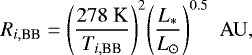
One of the first to reach a fundamental result in this field was Wisdom (1980) who estimated the stability of dynamical systems for a non-linear Hamiltonian with two degrees of freedom. Using the approximate criterion of the zero-order resonance overlap for the planar circular-restricted three-body problem, he derived the following formula for the chaotic zone that surrounds the planet
 (2)
(2)
where Δa is the half width of the chaotic zone, μ the ratio between the mass of the planet and the star, and ap is the semi-major axis of the planet’s orbit.
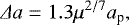
After this first analytical result, many numerical simulations have been performed in order to refine this formula. One particularly interesting expression regarding the clearing zone of a planet on a circular orbit was derived by Morrison & Malhotra (2015). The clearing zone, compared to the chaotic zone, is a tighter area around the orbit of the planet in which dust particles become unstable and from which are ejected rather quickly. The formulas for the clearing zones interior and exterior to the orbit of the planet are

The last result we want to highlight is the one obtained by Mustill & Wyatt (2012) using again N-body integrations and taking into account also the eccentricities e of the particles. Indeed, particles in a debris disk can have many different eccentricities even if the majority of them follow a common stream with a certain value of e. The expression for the half width of the chaotic zone in this case is given by
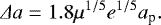 (5)
(5)
The chaotic zone is thus larger for greater eccentricities of particles. Equation (5) is only valid for values of e greater than a critical eccentricity, ecrit, given by
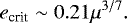 (6)
(6)
For e< ecrit this result is not valid anymore and Eq. (2) is more reliable. Even if each particle can have an eccentricity due to interactions with other bodies in the disk, such as for example collisional scattering or disruption of planetesimals in smaller objects resulting in high e values, one of the main effects that lies beneath global eccentricity in a debris disk is the presence of a planet on eccentric orbit. Mustill & Wyatt (2009) have shown that the linear secular theory gives a good approximation of the forced eccentricity ef even for eccentric planet and the equations giving ef are:
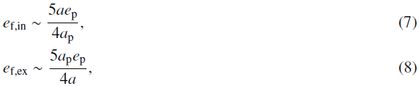
where ef, in and ef, ex are the forced eccentricities for planetesimals populating the disk interior and exterior to the orbit of the planet, respectively; ap and ep are, as usual, semi-major axis and eccentricity of the planet, while a is the semi-major of the disk. We note that such equations arise from the leading-order (in semi-major axis ratio) expansion of the Laplace coefficients, and hence are not accurate when the disk is very close to the planet.
It is common to take the eccentricities of the planet and disk as equal, because this latter is actually caused by the presence of the perturbing object. Such approximation is also confirmed by Eqs. (7) and (8). Indeed, the term 5∕4 is balanced by the ratio between the semi-major axis of the planet and that of the disk since, in our assumption, the planet gets very close to the edge of the belt and thus the values of ap are not so different from that of a, giving ef ~ ep.
Other studies, such as the ones presented in Chiang et al. (2009) and Quillen & Faber (2006), investigate the chaotic zone around the orbit of an eccentric planet and they all show very similar results to the ones discussed here above. However, in no case does the eccentricity of the planet appear directly in analytical expressions, with the exception of the equations presented in Pearce & Wyatt (2014) that are compared with our results in Sect. 5.2.
5.2 Numerical simulations
All the previous equations apply to the chaotic zone of a planet moving on a circular orbit. When we introduce an eccentricity ep , the planet varies its distance from the star. Recalling all the formulations for the clearing zone presented in Sect. 5.1 we can see that it always depends on the mean value of the distance between the star and the planet, ap , that is assumed to be almost constant along the orbit.
The first part of our analysis considers one single planet as the only responsible for the lack of particles between the edges of the inner and external belts. We show that the hypothesis of circular motion is not suitable for any system when considering masses under 50 MJ . For this reason, the introduction of eccentric orbits is of extreme importance in order to derive a complete scheme for the case of a single planet.
In order to account for the eccentric case we have to introduce new equations. The empirical approximation that we use (and that we support with numerical simulations) consists in starting from the old formulas (2) and (5) suitable for the circular case and replace the mean orbital radius, ap , with the positions of apoastron, Q, and periastron, q, in turn. We thus get the following equations
 (9) (10)
which replace Wisdom formula (2), and
 (11) (12)
which replace Mustill & Wyatt’s Eq. (5) and in which we choose to take as equal the eccentricities of the particles in the belt and that of the planet, e = ep. The substitution of ap with apoastron and periastron is somehow similar to considering the planet as split into two objects, one of which is moving on circular orbit at the periastron and the other on circular orbit at apoastron, and both with mass Mp .
In parallel with this approach, we performed a complementary numerical investigation of the location of the inner and outer limits of thegap carved in a potential planetesimal disk by a massive and eccentric planet orbiting within it to test the reliability of the analytical estimations in the case of eccentric planets.
We consider as a test bench a typical configuration used in numerical simulations with a planet of 1 MJ around a star of 1 M⊙ and two belts, one external and one internal to the orbit of the planet, composed of massless objects. The planet has a semi-major axis of 5 AU and eccentricities of 0, 0.3, 0.5, and 0.7 in the four simulations. We first perform a stability analysis of random sampled orbits using the frequency map analysis (FMA; Marzari 2014a). A large number of putative planetesimals are generated with semi-major axis a uniformly distributed within the intervals ap + RH < a < ap + 30RH and ap − 12RH < a < ap − RH, where RH is the radius of the Hill’s sphere of the planet. The initial eccentricities are small (lower than 0.01), meaning that the planetesimals acquire a proper eccentricity equal to the one forced by the secular perturbations of the planet. This implicitly assumes that the planetesimal belt was initially in a cold state.
The FMA analysis is performed on the non-singular variables h and k, defined as h = esinϖ and k = ecosϖ, of each planetesimal in the sample. The main frequencies present in the signal are due to the secular perturbations of the planet. Each dynamical system composed of planetesimal, planet, and central star is numerically integrated for 5 Myr with the RADAU integrator and the FMA analysis is performed using running time windows extending for 2 Myr. The main frequency is computed with the FMFT high-precision algorithm described in Laskar (1993) and Šidlichovský & Nesvorný (1996). The chaotic diffusion of the orbit is measured as the logarithm of the relative change of the main frequency of the signal over all the windows, cs . The steep decrease in the value of cs marks the onset of long-term stability for the planetesimals and it outlines the borders of the gap sculpted by the planet.
This approach allows a refined determination of the half width of the chaotic zone for eccentric planets. We term the inner and outer values of semi-major axis of the gap carved by the planet in the planetesimal disk ai and ao , respectively. For e = 0, we retrieve the values of ai and ao that can be derived from Eq. (2) even if ao is slightly larger in our model (6.1 AU instead of 5.9 AU). For increasing values of the planet eccentricity, ai moves insidewhile ao shifts outwards, both almost linearly. However, this trend is in semi-major axis while the spatial distribution of planetesimals depends on their radial distance.
For increasing values of ep, the planetesimals eccentricities grow as predicted by Eqs. (7) and (8) and the periastron of the planetesimals in the exterior disk moves inside while the apoastron in the interior disk moves outwards. As a consequence, the radial distribution trespasses ai and ao reducing the size of the gap. To account for this effect, we integrated the orbits of 4000 planetesimals for the interior disk and just as many for the exterior disk.
The bodies belonging to the exterior disk are generated with semi-major axis a larger than ao while for the interior disk a is smaller than ai. After a period of 10 Myr, long enoughfor their pericenter longitudes to be randomized, we compute the radial distribution. This will bedetermined by the eccentricity and periastron distributions of the planetesimals forced by the secular perturbations. In Fig. 1 we show the normalized radial distribution for ep = 0.3. At the end of the numerical simulation the radial distribution extends inside ao and outside ai.
The inner and outer belts are detected by the dust produced in collisions between the planetesimals. There are additional forces that act on the dust, like the Poynting-Robertson drag, slightly shifting the location of the debris disk compared to the radial distribution of the planetesimals. However, as a first approximation, we assume that the associated dusty disk coincides with the location of the planetesimals. In this case the outer and inner borders d2 and d1 of the external and internal disk, respectively, can be estimated as the values of the radial distance for which the density distribution of planetesimals drops to 0. Alternatively, we can require that the borders of the disk are defined as being where the dust is bright enough to be detected, and this may occur when the radial distribution of the planetesimals is larger than a given ratio of the peak value, fM , in the density distribution.
We arbitrarily test two different limits, one of 1∕3 fM and the other of 1∕4 fM , for both the internal and external disks. In this way, the low-density wings close to the planet on both sides are cut away under the assumption that they do not produce enough dust to be detected.
The d2 and d1 outer and inner limits of the external and internal disks are given in all three cases (0, 1∕3, and 1∕4) in Tables 1 and 2 for each eccentricity tested. The first three columns report the results of our simulations and are compared to the estimated values of the positions of the belts (last two columns) that we obtained in the first place, calculating the half width of the chaotic zone from Eqs. (10) and (12) for the inner belt and Eqs. (9) and (11) for the outer one, and then we use the relations
 (13) (14)
obtaining, in the end, d1 and d2.
We plot the positions of the two belts against the eccentricity for a cut-off of one third in Fig. 2. As we can see, results from simulations are in good agreement with our approximation. Particularly, we note how Wisdom is more suitable for eccentricities up to 0.3 (result that has already been proposed in a paper by Quillen & Faber (2006) in which the main conclusion was that particles in the belt do not feel any difference if there is a planet on circular or eccentric orbit for ep ≤ 0.3). For greater values of ep, Eqs. (11) and (12) also give reliable results.
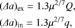
In Pearce & Wyatt (2014) a similar analysis is discussed regarding the shaping of the inner edge of a debris disk due to an eccentric planet that orbits inside the latter. As known from the second Kepler’s law, the planet has a lower velocity when it orbits near apoastron and thus it spends more time in such regions. Thus, they assumed that the position of the inner edge is mainly influenced by scattering of particles at apocenter in agreement with our hypothesis. Using the Hill stability criterion they obtain the following expression for the chaotic zone,
 (15)
(15)
where RH,Q is the Hill radius for the planet at apocenter, given by
![Mathematical equation: $ R_{\textrm{H}, Q}\sim a_{\textrm{p}}(1+e_{\textrm{p}})\left[\frac{M_{\textrm{p}}}{(3-e_{\textrm{p}})M_*}\right]^{1/3}\cdot$](/articles/aa/full_html/2018/03/aa31426-17/aa31426-17-eq11.png) (16)
(16)
Comparing Δaext to Eqs. (9), (11), and (15) for a planet of 1 MJ that orbits around a star of 1 M⊙ with a semi-major axis of ap = 5 AU (the typical values adopted in Pearce & Wyatt 2014) and eccentricity ep = 0.3, we obtain results that are in good agreement and differ by 15%. For the same parameters but higher eccentricity (ep = 0.5) the difference steeply decreases down to 2%. Thus, even if our analysis is based on different equations with respect to Eq. (15) the clearing zone that we obtain is in good agreement with values as expected by Pearce & Wyatt (2014), further corroborating our assumption for planets on eccentric orbits.
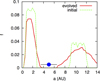 |
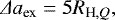
Fig. 1 Numerical simulation for a planet of 1 MJ around a star of 1 M⊙ with a semi-major axis of 5 AU and eccentricity of 0.3. We plot the fraction of bodies that are not ejected from the system as a function of the radius. Green lines represent the stability analysis on the radial distribution of the disk. Red lines represent the radial distributions of 4000 objects. |
Position of the inner belt.
Position of the outer belt.
 |
Fig. 2 Position of the inner (up) and external (down) belts for cuts off of one third. |
5.3 Dataanalysis
Once we have verified the reliability of our approximations, we proceed with analyzing the dynamics of the systems in the sample.
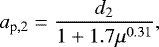
The first assumption that we tested is of a single planet on a circular orbit around its star. We use the equations for the clearing zone of Morrison & Malhotra (3) and (4). We vary the mass of the planet between 0.1 MJ, that is, Neptune/Uranus sizes, and 50 MJ in order to find the value of Mp, and the corresponding value of ap, at which the planet would sweep an area as wide as the gap between the two belts. 50 MJ represents the approximate upper limit of applicability of the equations, since they require that μ is much smaller than1. Since  , knowing Mp, we can obtain the semi-major axis of the planet by
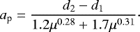 (17)
(17)
With this starting hypothesis we cannot find any suitable solution for any system in our sample. Thus objects more massive than 50 MJ are needed to carve out such gaps, but they would clearly lie well above the detection limits.
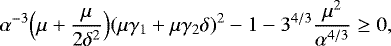
Since we get no satisfactory results for the circular case, we then consider one planet on an eccentric orbit. We use the approximation illustrated in the previous paragraph with one further assumption: we consider the apoastron of the planet as the point of the orbit nearest to the external belt while the periastron as the nearest point to the inner one. We let again the masses vary in the range [0.1, 50] MJ and, from Eqs. (9)–(12), we get the values of periastron and apoastron for both Wisdom and Mustill & Wyatt formulations, recalling also Eqs. (13) and (14). Therefore, we can deduce the eccentricity of the planet through
 (18)
(18)
Equation (5) contains itself the eccentricity of the planet ep , that is our unknown. The expression to solve in this case is
 (19)
(19)
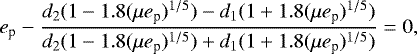
for which we found no analytic solution but only a numerical one. We can now plot the variation of the eccentricity as a function of the mass.We present two of these graphics, as examples, in Fig. 3.
In each graphic there are two curves, one of which represents the analysis carried out with the Wisdom formulation and the other with Mustill& Wyatt expressions. In both cases, the eccentricity decreases with increasing planet mass. This is an expected result since a less massive planet has a tighter chaotic zone and needs to come closer to the belts in order to separate them of an amount d2 − d1, that is fixedby the observations (and vice versa for a more massive planet that would have a wider Δa). Moreover, we note that the curve that represents Mustill & Wyatt’s formulas decreases more rapidly than Wisdom’s curve. This is due to the fact that Eq. (5) also takes into account the eccentricity of the planetesimals (in our case e = ep) and thus Δa is wider.
Comparing the graphics of the two systems, representative of the general behavior of our targets, we note that whereas for HD 35114, for increasing mass, the eccentricity reaches intermediate values ( ≤0.4), HD1466 needs planets on very high eccentric orbits even at large masses ( ≥0.6). From Table C.2, the separation between the belts in HD35114 is of ~86 AU whereas in HD1466 this is only ~40 AU. We can then wonder why in the first system planets with smaller eccentricity are needed to dig a gap larger than the one in the second system. The explanation regards the positions of the two belts: HD35114 has the inner ring placed at 6 AU whereas for HD1466 it is at 0.7 AU. From Eqs. (2) and (5) we obtain a chaotic zone that is larger for further planets since it is proportional to ap .
From the previous discussion, we deduce that many factors in debris disks are important in order to characterize the properties of the planetary architecture of a system: first of all the radial extent of the gap between the belts (the wider the gap, the more massive and/or eccentric are the planets needed); but also the positions of the belts (the closer to the star, the more difficult to sculpt) and the mass of the star itself.
For most of our systems the characteristics of the debris disks are not so favorable to host one single planet since we would need very massive objects that have not been detected. For this reason we now analyze the presence of two or three planets around each star.
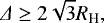
Before considering multiple planetary systems, however, we want to compare our results with the detection limits available in the sample and obtained as described in Sect. 4.2. We show, as an example, the results for HD 35114 and HD 1466 in Fig. 4 in which we plot the detection limits curve, the positions of the two belts (the vertical black lines) and three values of the mass. From the previous method we can associate a value of ap and ep to each value of the mass, noting that, as mentioned above, Wisdom gives more reliable results for ep ≤ 0.3, whereas Mustill & Wyatt for ep > 0.3. Moreover, we choose three values of masses because they represent well the three kinds of situation that we could find: for the smallest mass the planet is always below the detection limits and so never detectable; for intermediate mass the planet crosses the curve and thus it is detectable at certain radii of its orbit and undetectable at others (we note however, that the planet spends more time at apoastron than at periastron meaning that it is more likely detectable in this latter case); the higher value of Mp has only a small portion of its orbit (the area near to the periastron) that is hidden under the curve and thus undetectable.
We notethat in both figures there is a bump in the detection limit curves: this is due to the passage from the deeper observations done with IFS that has field of view ≤0.8 arcsec to the IRDIS ones that are less deep but cover a greater range of distances (up to 5.5 arcsec).
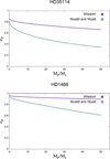 |
Fig. 3 ep vs. Mp for HD 35114 (up) and HD 1466 (down). |
 |
Fig. 4 SPHERE detection limits for HD 35114 (up) and HD 1466 (down). The bar plotted for each Mp represents the interval of distances covered by the planet during its orbit, from a minimum distance (periastron) to the maximum one (apoastron) from the star. The two vertical black lines represent the positions of the two belts. Projection effects in the case of significantly inclined systems are not included. |
6 Dynamical predictions for two and three planets
6.1 General physics
In order to study the stability of a system with two planets, we have to characterize the region between the two. From a dynamical point of view, this area is well characterized by the Hill criterion. Let us consider a system with a star of mass M* , the inner planet with mass Mp,1, semi-major axis of ap,1, and eccentricity ep ,1 , and the outer one with mass Mp,2, semi-major axis ap,2 and eccentricity ep ,2 . In the hypothesis of small planet masses, that is, Mp,1 ≪ M*, Mp ,2 ≪ M* and Mp ,2 + Mp,1 ≪ M*, the system will be Hill stable (Gladman 1993) if
 (20)
(20)
where μ1 and μ2 are the ratio between the mass of the inner/outer planet and the star respectively, α = μ1 + μ2, 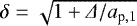 with Δ = ap,2 − ap,1 and, at the end,
 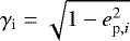 with i = 1, 2.
If the two planets in the system have equal mass, the previous Equation, taking Mp ,2 = Mp,1 = Mp and μ = Mp∕M*, can be rewritten in the form
 (21)
(21)
and substituting the expressions for α, δ, Δ, and γi we obtain
 (22)
(22)
Thus, the dependence of the stability on the mass of the two planets, in the case of equal mass, is very small since it appears only in the third term of the previous equation in the form μ2∕3 , with μ ≪ 1 and μ ≥0, and, for typical values, it is two orders of magnitude smaller than the first two terms. The leading terms that determine the dynamics of the system are the eccentricities ep,1 and ep,2. For this reason, we expect that small variation in the eccentricities will lead to great variation in mass.
A further simplification to the problem comes when we consider two equal-mass planets on circular orbits. In this case the stability Eq. (20) takes the contracted form
 (23)
(23)
where Δ is the difference between the radii of the planets’ orbits and RH is the planets mutual Hill radius that, in the general situation, is given by
 (24)
(24)
In the following, we investigate both the circular and the eccentric cases with two planets of equal mass.
The lastcase that we present is a system with three coplanar and equal-mass giant planets on circular orbits. The physics follows fromthe previous discussion since the stability zone between the first and the second planet, and between the second and the third is again well described by the Hill criterion. Once fixed, the inner planet semi-major axis ap ,1 , the semi-major axis of the second, and third planets is given by
 (25)
(25)
where the K value that ensures stability is a constant that depends on the mass of the planets and RH i,i+1 is the mutual Hill radius between the first and the second planets for i = 1 and between the second and the third for i = 2. K produces parametrization curves, called K-curves, that are weakly constrained. However, we can associate to K likely values that give us a clue on the architecture of the system. Following Marzari (2014a), the most used values of K for giant planets are:
-
K ~ 8 for Neptune-size planets;
-
K ~ 7 for Saturn-size planets;
-
K ~ 6 for Jupiter-size planets.
There is no analysis in the literature that gives analytical tools to explore the case of three or more giant planets with different masses and/or eccentric orbits. Thus, further investigations are merited even if they go beyond the scope of this work.
As we see in the following Sections, once we have established the stability of a multi-planetary system, we apply again the equations for the chaotic/clearing zone derived previously for a single planet as a criterion to describe the planet-disk interaction. However, for two and three planets, more complex dynamical effects due to mean motion and secular resonances may change the expected positions of the edges. We have compared our analytical predictions with the results obtained by Moro-Martín et al. (2010) who performed numerical simulations in four systems (HD 128311, HD 202206, HD 82943, and HR 8799) with known companions in order to determine the positions of the gap. While the outer edge of the inner belt is well reproduced by the formulas we have exploited, the inner edge of the outer belt is slightly shifted farther out for each system in the numerical modeling. This is in part related to the stronger and more stable mean motion resonances in the single-planet case. A full investigation of this problem is complex since the parameter space is wide as both the mass and eccentricity of the planets may change. However, we are interested in a first-order study and the differences due to the dynamical models are compatible with the error bars on the positions of the belts. Since we want only to give a method to obtain a rough estimation of possible architectures of planetary systems, such corrections are not included in this paper but we stress that deeper analyses are needed to obtain stronger and more precise conclusions.
6.2 Dataanalysis
6.2.1 Two and three planets on circular orbits
The first kind of analysis that we perform consists in taking into account two coplanar planets on circular orbits. In this case, between the two belts the system is divided into three different zones from a stability point of view. The first one extends from the outer edge of the internal disk to the inner planet and it is determined from interaction laws between two massive bodies (the star and the planet) and N massless objects. The second zone is included between the inner and the outer planets and is dominated by the Hill’s stability. Eventually, the third zone goes from the outer planet to the inner edge of the external belt and is an analog of the first one.
From Eq. (23) we note that a system with two planets is stable if Δ = ap,2 − ap,1 is greater or equal to a certain quantity. However, since we do not observe any amount of dust grains in the region between the planets, we expect it to be completely unstable for small particles. The condition needed to reach such a situation is called max packing, whereby the two planets are made to become as close as possible whilst remaining a stable system. Therefore, the max packing condition is satisfied by the equation
 (26)
(26)
The other two equations that we need are the ones of Morrison & Malhotra, Eqs. (3) and (4), from which we obtain ap,1 and ap,2 in the form
 (27)
(27)
 (28)
(28)
and substituting in Eq. (26) we get
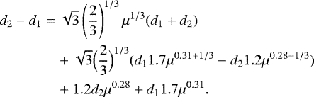 (29)
(29)
This is a very complex equation to solve for Mp and we need to make some simplifications. We note that all the exponents of μ have very similar values with the exception of the two μ in the third term on the right side of the equation, in which, however, the exponents are about double of all others. Thus, we choose μ0.31 as a mean value, and μ0.62 in the third term for both terms in the brackets. Calling x = μ0.31 we have now to solve the quadratic equation
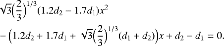 (30)
(30)
We can finally obtain the value of Mp, given the positions of the two belts and the mass of the star
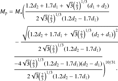 (31)
(31)
The numerical outcomes of the equation show that this formula is reliable. We recall that our equations are valid only for μ ≪ 1, thus we choose again as upper limit 50 MJ and arbitrarily we consider only masses bigger than 0.1 MJ. In the case of two equal-mass planets on coplanar circular orbits we obtain satisfying results only in 8 cases out of 35 presented in Table C.2.
The case of three planets of equal mass on circular orbits is quite similar and of particular interest. Indeed, systems of three (or more) lower-mass planets may be more likely sculptors than two massive planets on eccentric orbits that will be considered in the following section, both because the occurrence rate of lower-mass planets is higher than Jovian planets (at least in regions close to the star) as seen, for example, from Kepler (Howard et al. 2012) or RV (Mayor et al. 2011; Raymond et al. 2012) planet occurrence rates, and because the disk would not have to survive planet-planet scattering without being depleted (Marzari 2014b).
For the three-planet case, we have to consider four zones of instability for the particles: the first and the fourth are determined by the inner and the outer planet assuming Eqs. (3) and (4) respectively, while the second and the third by the Hill criterion.
From Eq. (25), we can express the mutual dependence between the positions of the three planets as
 (32) (33)
We can obtain ap,2 from Eq. (32) and substituting it in Eq. (33) we get
 (34)
(34)
where ap,1 and ap,3 are determined by Eqs. (3) and (4). The final expression to solve for Mp becomes
 (35)
(35)
In analogy with the previous cases, we impose a lower limit on the mass at 0.1 MJ but we have a further constraint on the upper one since values of K are valid only up to some Jupiter masses. Thus we take as upper limit for the three planets model 15 MJ . The values of K are the ones described in the previous paragraph, with K = 8 for masses up to 0.3 MJ , K = 7 for masses in the range [0.3, 0.9]MJ and K = 6 for Mp ≥ 1MJ. For three equal-mass planets on circular coplanar orbits we obtain more encouraging results since with such configuration the gap could be explained in 25 cases out of 35. Results of the analysis of two and three planets on circular orbits are shown in Fig. 5.
Together with the values of the masses for each system suitable to host two and/or three planets on circular orbits, we indicate the detectability of such planets, comparing their masses and semi-major axis with SPHERE detection limits. The condition for detectability in this case is that at least one object in the two- or three-planet model is above the detection limits curve. However, as mentioned in Sect. 4, inclination of the disk may affect the detectability of the putative planets due to projection effects. Indeed, objects that are labeled as detectable in Fig. 5 are always observable only if the disk is face-on. With increasing inclination, the chance of detecting the planets decreases. Whereas for the two-planet case the probability of detecting at least the outer objects is usually very high due to the big masses obtained, for the three-planet case, half of the systems labeled as detectable are indeed observable only 50% of the time (the worst case is for the outer putative planet of HD 133863 which would be detectable only 37% of the time).
With the exception of very few systems, such as for example HD 174429, HR 8799, HD 206893, and HD 95086, no giant planets or brown dwarfs have been discovered between the two belts in the systems of our selected sample using direct imaging techniques. Thus, we expect that if planets are indeed present, they must remain undetectable with our observations. In all systems, two planets on circular orbits would have been detected, since large masses are required. The situation improves significantly for the three-planet model because many systems can be explained with planets that would remain undetected. Therefore, in most cases, the assumption of three equal-mass planets on circular orbits is more suitable than the one with two planets withthe same characteristics.
Obviously in this paragraph we have made very restrictive hypotheses: circular orbits and equal-mass planetary systems. Varying these two assumptions would give many suitable combinations in order to explain what we do (or do not) observe.
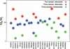 |
Fig. 5 Masses (Mp∕MJ) for the systems with two and three equal-mass planets on circular orbits: red circles represent a system with two planets that are detectable, while green and blue circles represent three planets detectable and undetectable, respectively. Since the equations are not fully correct for more massive planets, for the two-planet case we show only systems for which MP ≤ 50 MJ whereas for the three-planet case we show only systems for which MP ≤ 15 MJ. |
6.2.2 Two planets on eccentric orbits
The last model we want to investigate comprises two equal-mass planets on eccentric orbits. The system is again divisible into three regions of stability. The zone between the two planets follows the Hill criterion for the condition of max packing given by Eq. (22) with the equal sign. For the outer and inner regions the force is exerted by the planets on the massless bodies in the belts. This time, however, we use Wisdom and Mustill & Wyatt expressions instead of Morrison & Malhotra’s, suitable only for the circular case. Precisely, we apply the equation of Wisdom for eccentricities up to 0.3 whereas for greater values of ep we use Mustill & Wyatt, together with the substitution of ap with apoastron and periastron of the planets.
We have four different situations:
-
if ep,1 and ep,2 are both ≤0.3, then we used equations of Wisdom (9) and (10), from which we obtain ap,1 and ap,2 in the form

-
if ep,1 ≤ 0.3 and ep,2 > 0.3 we apply at the inner planet the equation of Wisdom (10) and at the outer one Eq. (11) from Mustill & Wyatt, thus obtaining

-
if ep,1 > 0.3 and ep,2 ≤ 0.3 we have the opposite situation with respect to the one described above, thus we use Mustill & Wyatt for the inner planet and Wisdom for the outer one

-
if ep,1 and ep,2 are both > 0.3 we use Mustill & Wyatt for the two planets

Thus, depending on the values of ep,1 and ep,2 we substitute in Eq. (22) expressions of ap,1 and ap,2 as obtained above. Varying the masses in the range [0.1, 25] MJ, we obtain the respective values of eccentricities for the two planets. We note that we are implicitly assuming that the two eccentric planets will remain on the same orbits for their whole lifetime whereas, in reality, their eccentricities will fluctuate. This may imply lower masses of the two planets required to dig the gap as the systems are unlikely to be observed at the peak of an eccentric cycle.
We show in Fig. 6 the results of this analysis for HD 35114. For each system, we obtain a set of suitable points identified by the three coordinates [ep,1, ep,2, Mp] (we recall that the two planets in the system have the same mass). Therefore, we prepare a grid with the two values of eccentricities on the axes and we associate a scale of colors to the mass range (see Fig. 6). Moreover, in order to determine which planets would have been detected, we confront, as always, values of semi-major axis and mass with the detection limit curves and use as a criterion of detectability, the condition in which at least one of the two planets is above the curve even just in partial zones of its orbit (see Fig. 6).
In the graphics, we indicate with a black line the approximate detection limits: points above the line are undetectable whereas points below are detectable. From Fig. 6 it is clearly visible how mass (and thus detectability) decreases with increasing eccentricities. Moreover, small variations of ep ,1 and/or ep ,2 cause a great damp in mass since, as already mentioned above, the stability depends very little on the mass of the two planets.
From this study emerges the fact that the apparent lack of giant planets in the sample of systems analyzed can easily be explainedby taking quite eccentric planets of moderate masses that lay beneath the detection limit curve. Indeed, large eccentricities are common features of exoplanets (Udry & Santos 2007) and thus we must not abandon the hypothesis that gaps between two planetesimal belts can be dug by massive objects that surround the central star.
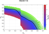 |
Fig. 6 Analysis for HD 35114 with two equal-mass planets on eccentric orbits. On the axes, the eccentricity of the inner (e1 ) and outer (e2) planets. The graduation of colors represents values of Mp∕MJ. The black line represents the approximate detection limits: points above the line are undetectable whereas points below are detectable. The discontinuity at e = 0.3 is due to the passage from Wisdom’s equation to Mustill and Wyatt’s one. |
7 Particularly interesting systems
7.1 HD 106906
HD 106906AB is a close binary system (Lagrange et al. 2016) where both stars are F5 and are located at a distance of 91.8 pc. They belong to the Lower Centaurus Crux (LCC) group, which is a subgroup of the Scorpius-Centaurus (Sco-Cen) OB association. Bailey et al. (2014) detected a companion planet, HD 106906 b, of 11 ± 2 MJ located at ~650 AU in projected separation and an asymmetric circumbinary debris disk nearly edge-on resolved by different instruments (see Appendix B). The evident asymmetries of the disk could suggest interactions between the planet and the disk (Rodet et al. 2017; Nesvold et al. 2017). The gap in the disk is located between 13.1 AU and 56 AU and the detected companion orbits far away from this area. Since the gap is quite small, we find promising results for one or more undetected companions. As mentioned in Sect. 5, it is not possible to explain the gap with a single planet (with MP ≤ 50 MJ) on a circular orbit. In Fig. 7 we show ep vs. Mp for one eccentric planet to be responsible for the empty space between the belts: we do not need particularly high eccentricity even at low masses. Thus the gap, together with the non detection of another companion (besides HD 106906 b), could be explained by a single planet on an eccentric orbit as shown in Fig. 8. For example, a planet with a mass of 1 MJ , semi-major axis ap ~ 45 AU and a reasonable value of eccentricity, ep ~ 0.4, would be able to dig the gap and be undetectable at the same time. However, we can consider a more complex architecture. In Figs. 8 and 9 we show two and three equal-mass planets on circular orbits and two planets on eccentric orbits: whereas two planets on circular orbits would have been easily detected, two of the planets of the three-circular-planets case are undetectable and the farthest one is very close to detection limits. Moreover, combining the orbital parameters of the third planet with the projection effects due to the inclination of the disk (i = 85°), we obtain that it would be detectable only 55% of the time. Two planets on eccentric orbits with eccentricities ≥0.2 could be under the detection limit curve.
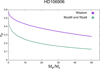 |
Fig. 7 One planet on an eccentric orbit around HD 106906. |
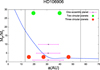 |
Fig. 8 Three different values of mass (1, 5, and 10 MJ) of putative planets with their respective semi-major axis and eccentricities and the detection limit curve for the HD 106906 system (pink lines) and two (green circles) and three (red circles) planets on circular orbits around HD 106906. |
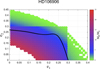 |
Fig. 9 Predictions and comparison with the SPHERE detection limits (black line) for the eccentric two-planet model for HD 106906. |
7.2 HD 174429 (PZ Tel)
HD 174429, or PZ Tel A, is a G9IV star member of the moving group β Pictoris. It is located at a distance of 49.7 pc and an M brown dwarf companion was discovered independently by Mugrauer et al. (2010) and Biller et al. (2010) to orbit this star at a separation of ~25 AU on a very eccentric orbit (e > 0.66, Maire et al. 2016). The mass of PZ Tel B varies in the range [20, 40] MJ depending on the age of the system (Ginski et al. 2014; Schmidt et al. 2014).
From SED fitting, Chen et al. (2014) found that the debris disk of PZ Tel is better represented by two components. However, excesses in the near-IR typical of the warm component were never observed and the small deviation from the SED of the star could be attributed to the presence of the brown dwarf. Regarding the cold component, Chen et al. (2014) obtained a temperature of 39 K that, together with the Γ correction, places the belt at 317.5 AU. In spite of this, Riviere-Marichalar et al. (2014) rejected the hypothesis of the presence of a debris disk because they did not find infrared excesses with Herschel/PACS at 70, 100, and 160 μm.
Since the literature on this disk is relatively scarce and discordant, we want to apply our method to the known companion in order to check if it can add constraints on the existence of the disk. The orbit of the brown dwarf is still a matter of debate but we know that it has to be very eccentric. Thus, we can use 30 MJ as a mean value for themass and the three best orbits presented in Table 13 of Maire et al. (2016) together with the formulation for one single planet on an eccentric orbit. We obtained as a result that, for the first two orbits, the planet does not cross the external disk, placing the edge at ~250 AU for the first one (very near to our estimated inner edge) and at ~150 AU in the second (leaving some free dynamical space). The third orbit, instead, would cross the disk and destroy its configuration. Thus, we cannot completely exclude the presence of a cold debris disk component.
7.3 HR 8799
HR 8799 is a γ Dor-type variable star (Gray & Kaye 1999). The most incredible characteristic of HR 8799 is that it hosts four giant planets in the gap between the two components of the disk, with masses in the range [5, 7] MJ and distances in the range [15, 70] AU (Marois et al. 2010b). Moreover, the disk around this star is spatially resolved in its outer component in far IR and millimeter wavelengths (Su et al. 2009; Booth et al. 2016) and, besides the warm and cold belts placed at ~9 AU and ~200 AU, respectively, it shows an extended halo up to 2000 AU. Our dynamical analysis takes into account three planets, meaning that we are not able to determine the precise dynamical behavior of HR 8799- b, c, d, and e. However, we can make some estimates based on our results. We show the results for three planets on circular orbits in Fig. 10, which are the ones that come closer to the real architecture of HR 8799 represented by the pink circles in the same figure (Konopacky et al. 2016, indeed, orbits with large eccentricities are not favored by current analyses). We find three equal-mass planets of 6.6 MJ that are similar to the estimated masses of HR 8799 bcde. Thus it seems that this system, in order to be stable, must be dynamically full and even more packed to host four giant planets, and mean motion resonances, that are not included in our analysis, may be at work (Esposito et al. 2016; Goździewski & Migaszewski 2014).
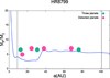 |
Fig. 10 Analytical results for three planets on circular orbits (green circles) and the actual four detected planets (pink circles) around HR 8799. |
7.4 HR 4796
HR 4796A is a A0 star and it is part of the TW Hydra kinematic group. It is part of a binary system with the M2 companion HR 4796B orbiting at a projected separation of 560 AU. The debris disk around this star is resolved in scattered light and near IR. The images show a thin, highly inclined ring with an eccentricity of ~0.06 at ~75 AU from the star (Kastner et al. 2008). The eccentricity of the disk and the sharpness of its inner edge seems to point to the presence of a planet orbiting right inside the gap. However, no companion has been detected so far (Milli et al. 2017b). Thus we would expect a planet with small mass under the detection limits curve or with high eccentricity such that it passes, at some point during its orbit, into areas sufficiently near to the star, even if the second hypothesis should imply a higher forced eccentricity of the disk. Comparing Figs. 11 and 12 we obtain that objects with masses ≤2 MJ are undetectable, but, at the same time, they need high eccentricities ( ≥0.6). Moreover, if we consider Eq. (8) for the forced eccentricity exerted by the planet on the belt, we should expect an eccentricity of the latter of ~0.1, requiring masses ≥50 MJ , well above the detection limit curve. Thus, we consider a more complex configuration with two and three planets (Figs. 12 and 13). No result was found for two planets on circular orbits, whereas, for three companions, we find masses of 8.7 MJ each. In thislast scenario, two of the three planets would be detected (even taking into account the inclination of the disk, i = 75°, the farthest putative planet would be always detectable) so we move to consider the case of two planets on eccentric orbits. Since for this kind of analysis, as explained in Sect. 6, the eccentricities of the two planets have a greater importance than the masses, we finally find possible solutions to explain the gap with the presence of undetectable objects (see Fig. 13).
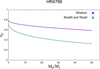 |
Fig. 11 One planet on an eccentric orbit around HR 4796. |
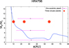 |
Fig. 12 Three different values of mass (1, 5, and 10 MJ) with their respective semi-major axis and eccentricities and the detection limits curve for the system (pink lines) and three planets on circular coplanar orbits around HR 4796 (red circles). |
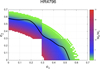 |
Fig. 13 Two planets on eccentric orbits around HR 4796 and comparison with detection limits (black line). |
8 Conclusions and perspectives
In this workwe studied systems that harbor two debris belts and a gap between them. The main assumption was that one or more planets are responsible for the gap. In a sample of 35 systems with double belts also observed as part of the SPHERE GTO survey we found no planet or brown dwarf within the gap, with the exception of HD 218396 (HR 8799), HD 174429 (PZ Tel), HD 206893, and HD 95086. We note that some systems in our sample have detected and/or candidate companions that however orbit outside the gap (Langlois et al., in prep.). The lack of planet detections within the belt may be due either to the dynamical and physical properties of the planets placing them below the detection limits of actual instruments, or to some complex mechanism by which such systems were born with two separate disk components (Kral et al. 2017a).
We focused on the first hypothesis and tested the detectability of different packed planetary systems which may carve the observed gap. We first investigated the presence of one single planet on a circular orbit and we found that for the systems in our sample most planets should have been detected or are too massive to be classified as planets.
Our next step was to consider a single planet in an eccentric orbit using the equations of Wisdom or Mustill & Wyatt for the chaotic zone of a planet on a circular orbit but replacing in the equations the semi-major axis of the planet with its periastron or apoastron to compute the border of the inner or outer belt, respectively. For larger eccentricities, the mass of the planet decreases slightly but extreme parameters are still required to model the double-belt structure. To have undetectable planets with masses beneath detection limits we predict values of ep greater than 0.7 in most systems. Thus, even if the hypothesis of one planet could be suitable in some cases, we tried a different approach assuming that the gap is created by a packed system of lower-mass planets. We have explored the case of two or three planets in the gap to see if we can explain the gap and the non-detection of planets by SPHERE. The first model considers two equal-mass planets on circular orbits, but even in this case, most of the planets should have been detected by SPHERE. The most promising scenario models the presence of the gap as due to the perturbations of either a system of three planets on circular orbits or two planets on eccentric orbits. In both these scenarios the planets would be undetected by SPHERE. In particular, the case with eccentric orbits shows that even a small variation in the eccentricity of one of the two planets leads to a drop in their masses, hiding them from possible detections.
We summarize our results in Table C.4. We show values of masses for the case of one, two, and three planets on circular orbits as found by our dynamical analysis. For the case of three planets, we indicate with an asterisk the undetectable objects. We show also results for masses and eccentricities for one and two planets on eccentric orbits: in eccentric cases, the orbital parameters are not univocally determined, because of the degeneracy between the mass and the eccentricity of the planet. Thus, for one single planet on an eccentric orbit, we show only the (MP, eP) values at the boundary between detectability and undetectability. The same criterion is applied in discerning values of (MP, e1, e2) for two planets on eccentric orbits. However, we have to apply a further selection in this case since, given a fixed value of the mass, different possible combinations of the eccentricities of the two planets are possible. Therefore, for each system, we choose to show only the combination for which values of e1 and e2 are similar.
We conclude our work noticing that, even if very few planets have been detected so far in the gap of double belts, we cannot rule out the hypothesis that the gap is indeed due to massive objects orbiting within it; one or two planets on circular orbits would have been revealed for each system, in contrast with our observations, and more complex architectures should be taken into account. Multiple planets systems with eccentric orbits may be responsible for these belts’ architectures as in the case of HR 8799 or the solar system.
This paper presents a quick method to estimate the masses and eccentricities of the planets in this packed configuration in order to gain a first glimpse at the possible architecture of the planetary system in the gap. Thanks to the analytical formulations we can easily obtain masses, semi-major axes, and eccentricities of planets responsible for the gap. When the SPHERE GTO program will be completed, the number of observed two-component disks will have more than doubled. All these systems will be suitable for this kind of analysis and a statistical study on the presence of planets between belts will be possible. Moreover, spatially resolved images such as those that are and will be provided by instruments like SPHERE, GPI, ALMA, and JWT will be of extreme importance in order to come to more complete and robust conclusions on debris disks, exoplanets, and their interactions.
Acknowledgements
SPHERE is an instrument designed and built by a consortium consisting of IPAG (Grenoble, France), MPIA (Heidelberg, Germany), LAM (Marseille, France), LESIA (Paris, France), Laboratoire Lagrange (Nice, France), INAF-Osservatorio di Padova (Italy), Observatoire de Geneve (Switzerland), ETH Zurich (Switzerland), NOVA (The Netherlands), ONERA (France) and ASTRON (The Netherlands) in collaboration with ESO. SPHERE was funded by ESO, with additional contributions from CNRS (France), MPIA (Germany), INAF (Italy), FINES (Switzerland) and NOVA (The Netherlands). SPHERE also received funding from the European Commission Sixth and Seventh Framework Programmes as part of the Optical Infrared Coordination Network for Astronomy (OPTICON) under grant number RII3-Ct-2004-001566 for FP6 (2004-2008),grant number 226604 for FP7 (2009-2012) and grant number 312430 for FP7 (2013-2016). This work has made use of the the SPHERE Data Centre, jointly operated by OSUG/IPAG (Grenoble), PYTHEAS/LAM/CESAM (Marseille), OCA/Lagrange (Nice) and Observtoire de Paris/LESIA (Paris). We thank P. Delorme and E. Lagadec (SPHERE Data Centre) for their efficient help during the data reduction process. We acknowledge financial support from the “Progetti Premiali” funding scheme of the Italian Ministry of Education, University, and Research. We acknowledge financial support from the Programme National de Planetologie (PNP) and the Programme National de Physique Stellaire (PNPS) of CNRS-INSU. This work has also been supported by a grant from the French Labex OSUG2020 (Investissements d’avenir - ANR10 LABX56). The project is supported by CNRS, by the Agence Nationale de la Recherche (ANR-14-CE33-0018; ANR-16-CE31-0013). Quentin Kral acknowledges funding from STFC via the Institute of Astronomy, Cambridge, Consolidated Grant. We thank the referee Dr. A. Mustill for useful comments.
Appendix A Γ correction
From images of resolved disks we know that outer components are placed farther away compared to the predicted blackbody positions (Pawellek et al. 2014). In Pawellek & Krivov (2015) they analyzed a sample of 32 systems resolved by Herschel/PACS and found a relation between the real radius of the disks and the blackbody radius.
Definingthe ratio between the two radii as Γ, they found that it depends on a certain power law of the luminosity of the star,
 (A.1)
(A.1)
They explored five different compositions of dust grains: 50% astrosilicates and 50% vacuum, 50% astrosilicates and 50% ice, 100% astrosilcates, 50% astrosilicates, and 50% carbon, and 100% carbon. With the exception of 100% astrosilicates, particles for which A = 8.26 and B = −0.55, they obtained similar values of A and B for each combination. We thus exclude pure astrosilicates and take mean values of the two parameters between the remaining compositions, A = 6 and B = −0.4.
The use of the Γ factor would be misleading for disks with high asymmetries or particular features such as extended halos that were, indeed, not considered by Pawellek & Krivov (2015) in their analysis. Moreover, the Γ correction is suitable only for systems with luminosity L*≥ L⊙.
Morales et al. (2016) reach similar conclusions, showing, for a sample of resolved systems with Herschel, that the position of the disk is better reproduced modeling the SED with dust grains composed of astrosilicates made of a mixture of dirty ice and pure water.
We show in Fig. A.1 how much the results of SED analysis with blackbody hypothesis (upper panel) and with correction Γ (lower panel) differ from data available in 17 (out of 19; we have to discard HD 61005 and HD 202917 because their luminosities are <L⊙) resolved systems for the outer belt. The error bars represent the extension of the disks from the inner edge Rin at the lower extremity to the outer edge Rout at the upper one. Some systems have disks with small error bars because they are best modeled by thin rings centered on the mid-radii of the belts.
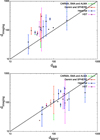 |
Fig. A.1 Position of the outer belts as obtained from SED analysis with hypothesis of blackbody (above) and with correction factor Γ (beneath) vs. positions obtained from resolved images. The black line represents the bisector, that is, when the two positions coincide. The vertical error bars represent instead the extension of the disk from its inner edge to its outer one. |
In the upper panel, we can see a consistent difference and a systematic upward shift between SED modeling and direct imaging data, with the blackbody fitting placing the belt indeed nearer to the star. This should not be a surprise since, as mentioned before, we expect that the disk is placed farther out when the particles do not behave like perfect absorbers/emitters. For these systems the situation improves applying the Γ correction, as shown in the lower panel.
We notethat some error in the SED fitting could also exist. Indeed, dust grains placed so far from the star have low temperatures (thus longer wavelengths) that are less constrained and more difficult to determine and only few photometric points are available. Moreover, discordances between SED and direct imaging analysis could be caused by other factors. For example, the resolved systems are analyzed at certain wavelengths depending on the instrumentation used and the disk will appear quite different for each value of λ whereas SED fitting identifies only the dust component. However, the fact that the Pawellek & Krivov (2015) correction, developed for a sample of targets observed with Herschel, holds reasonably well for a sample of objects resolved with different instruments/wavelengths indicates that such effects are not dominant in our sample.
Appendix B Spatially resolved systems
We list in Table B.1 the systems among the ones of our sample that were previously resolved in their farthest component by means of direct imaging. For each of such objects we show the instrument and the wavelengths at which the disk was resolved, the position a of the mean radius of the disk and its innerand outer edges Rin and Rout, the inclination i (measured from face on, in which case i = 0°) and the position angle PA. We note that the distances of the stars used in different papers may vary relative to each other and to distances used in this paper. For this reason we normalized the dimensions of the disks with distances listed in Table C.1. The only caveat is that this procedure should be entirely correct only when disk parameters are obtained directly from images and not from further modeling (such as SED modeling).
Spatially resolved systems.
Appendix C Additional tables
Stellar parameters for directly imaged systems with SPHERE.
Debris disk parameters for direct imaged systems with SPHERE.
Observations of the sample.
Values of masses and eccentricities needed to carve the gaps for the systems in the sample assuming one, two, or three planets.
References
- Apai, D., Janson, M., Moro-Martín, A., et al. 2008, ApJ, 672, 1196 [NASA ADS] [CrossRef] [Google Scholar]
- Bailey, V., Meshkat, T., Reiter, M., et al. 2014, ApJ, 780, L4 [Google Scholar]
- Baraffe, I., Chabrier, G., Barman, T. S., Allard, F., & Hauschildt, P. H. 2003, A&A, 402, 701 [NASA ADS] [CrossRef] [EDP Sciences] [Google Scholar]
- Beuzit, J.-L., Feldt, M., Dohlen, K., et al. 2008, in Ground-based and Airborne Instrumentation for Astronomy II, Proc. SPIE, 7014, 701418 [CrossRef] [Google Scholar]
- Biller, B. A., Liu, M. C., Wahhaj, Z., et al. 2010, ApJ, 720, L82 [NASA ADS] [CrossRef] [Google Scholar]
- Boccaletti, A., Abe, L., Baudrand, J., et al. 2008, in Adaptive Optics Systems, Proc. SPIE, 7015, 70151B [Google Scholar]
- Bonavita, M., Desidera, S., Thalmann, C., et al. 2016, A&A, 593, A38 [NASA ADS] [CrossRef] [EDP Sciences] [Google Scholar]
- Bonnefoy, M., Milli, J., Ménard, F., et al. 2017, A&A, 597, L7 [NASA ADS] [CrossRef] [EDP Sciences] [Google Scholar]
- Booth, M., Kennedy, G., Sibthorpe, B., et al. 2013, MNRAS, 428, 1263 [NASA ADS] [CrossRef] [Google Scholar]
- Booth, M., Jordan, A., Casassus, S., et al. 2016, MNRAS, 460, 10 [Google Scholar]
- Booth, M., Dent, W. R. F., Jordán, A., et al. 2017, MNRAS, 469, 3200 [NASA ADS] [CrossRef] [Google Scholar]
- Bowler, B. P. 2016, PASP, 128, 102001 [NASA ADS] [CrossRef] [Google Scholar]
- Buenzli, E., Thalmann, C., Vigan, A., et al. 2010, A&A, 524, L1 [NASA ADS] [CrossRef] [EDP Sciences] [Google Scholar]
- Carbillet, M., Bendjoya, P., Abe, L., et al. 2011, Experim. Astron., 30, 39 [Google Scholar]
- Chen, C. H., Mittal, T., Kuchner, M., et al. 2014, ApJ, 211, 25 [Google Scholar]
- Chiang, E., Kite, E., Kalas, P., Graham, J. R., & Clampin, M. 2009, ApJ, 693, 734 [Google Scholar]
- Churcher, L. J., Wyatt, M. C., Duchêne, G., et al. 2011, MNRAS, 417, 1715 [NASA ADS] [CrossRef] [Google Scholar]
- Claudi, R. U., Turatto, M., Gratton, R. G., et al. 2008, in Ground-based and Airborne Instrumentation for Astronomy II, Proc. SPIE, 7014, 70143E [Google Scholar]
- Delorme, P., Schmidt, T., Bonnefoy, M., et al. 2017, A&A, 608, A79 [NASA ADS] [CrossRef] [EDP Sciences] [Google Scholar]
- Desidera, S., Covino, E., Messina, S., et al. 2015, A&A, 573, A126 [NASA ADS] [CrossRef] [EDP Sciences] [Google Scholar]
- Dohlen, K., Langlois, M., Saisse, M., et al. 2008, in Ground-based and Airborne Instrumentation for Astronomy II, Proc. SPIE, 7014, 70143L [CrossRef] [Google Scholar]
- Esposito, T. M., Fitzgerald, M. P., Graham, J. R., et al. 2016, AJ, 152, 85 [NASA ADS] [CrossRef] [Google Scholar]
- Feldt, M., Olofsson, J., Boccaletti, A., et al. 2017, A&A, 601, A7 [NASA ADS] [CrossRef] [EDP Sciences] [Google Scholar]
- Fusco, T., Rousset, G., Sauvage, J.-F., et al. 2006, Opt. Exp., 14, 7515 [Google Scholar]
- Geiler, F., & Krivov, A. 2017, MNRAS, 468, 959 [NASA ADS] [CrossRef] [Google Scholar]
- Ginski, C., Schmidt, T. O. B., Mugrauer, M., et al. 2014, MNRAS, 444, 2280 [NASA ADS] [CrossRef] [Google Scholar]
- Gladman, B. 1993, Icarus, 106, 247 [NASA ADS] [CrossRef] [Google Scholar]
- Gladman, B., Kavelaars, J. J., Petit, J.-M., et al. 2001, AJ, 122, 1051 [NASA ADS] [CrossRef] [Google Scholar]
- Goździewski, K., & Migaszewski, C. 2014, MNRAS, 440, 3140 [NASA ADS] [CrossRef] [Google Scholar]
- Gray, R. O., & Kaye, A. B. 1999, AJ, 118, 2993 [NASA ADS] [CrossRef] [Google Scholar]
- Hines, D. C., Schneider, G., Hollenbach, D., et al. 2007, ApJ, 671, L165 [NASA ADS] [CrossRef] [Google Scholar]
- Howard, A. W., Marcy, G. W., Bryson, S. T., et al. 2012, ApJS, 201, 15 [NASA ADS] [CrossRef] [Google Scholar]
- Hughes, A. M., Wilner, D. J., Andrews, S. M., et al. 2011, ApJ, 740, 38 [NASA ADS] [CrossRef] [Google Scholar]
- Hung, L.-W., Duchêne, G., Arriaga, P., et al. 2015a, ApJ, 815, L14 [NASA ADS] [CrossRef] [Google Scholar]
- Hung, L. W., Fitzgerald, M. P., Chen, C. H., et al. 2015b, ApJ, 802, 138 [NASA ADS] [CrossRef] [Google Scholar]
- Janson, M., Brandt, T. D., Moro-Martín, A., et al. 2013, ApJ, 773, 73 [NASA ADS] [CrossRef] [Google Scholar]
- Janson, M., Quanz, S. P., Carson, J. C., et al. 2015, A&A, 574, A120 [NASA ADS] [CrossRef] [EDP Sciences] [Google Scholar]
- Kalas, P. G., Rajan, A., Wang, J. J., et al. 2015, ApJ, 814, 32 [NASA ADS] [CrossRef] [Google Scholar]
- Kanagawa, K. D., Muto, T., Tanaka, H., et al. 2016, PASJ, 68, 43 [NASA ADS] [Google Scholar]
- Kastner, J. H., Zuckerman, B., & Bessell, M. 2008, A&A, 491, 829 [NASA ADS] [CrossRef] [EDP Sciences] [Google Scholar]
- Kennedy, G. M., & Wyatt, M. C. 2014, MNRAS, 444, 3164 [NASA ADS] [CrossRef] [Google Scholar]
- Konopacky, Q. M., Marois, C., Macintosh, B. A., et al. 2016, AJ, 152, 28 [NASA ADS] [CrossRef] [Google Scholar]
- Kral, Q., Thébault, P., Augereau, J.-C., Boccaletti, A., & Charnoz, S. 2015, A&A, 573, A39 [NASA ADS] [CrossRef] [EDP Sciences] [Google Scholar]
- Kral, Q., Clarke, C., & Wyatt, M. 2017a, in Handbook of Exoplanets, eds. H. Deeg, & J. Belmonte (Springer, Cham) [Google Scholar]
- Kral, Q., Krivov, A. V., Defrere, D., et al. 2017b, Astron. Rev., 13, 69 [NASA ADS] [Google Scholar]
- Krivov, A. V. 2010, Res. Astron. Astrophys., 10, 383 [NASA ADS] [CrossRef] [Google Scholar]
- Lagrange, A.-M., Bonnefoy, M., Chauvin, G., et al. 2010, Science, 329, 57 [NASA ADS] [CrossRef] [PubMed] [Google Scholar]
- Lagrange, A.-M., Milli, J., Boccaletti, A., et al. 2012, A&A, 546, A38 [NASA ADS] [CrossRef] [EDP Sciences] [Google Scholar]
- Lagrange, A. M., Langlois, M., Gratton, R., et al. 2016, A&A, 586, L8 [NASA ADS] [CrossRef] [EDP Sciences] [Google Scholar]
- Laskar, J. 1993, Physica D, 67, 257 [Google Scholar]
- Lebreton, J., Augereau, J.-C., Thi, W.-F., et al. 2012, A&A, 539, A17 [NASA ADS] [CrossRef] [EDP Sciences] [Google Scholar]
- Levison, H. F., Morbidelli, A., Van Laerhoven, C., Gomes, R., & Tsiganis, K. 2008, Icarus, 196, 258 [NASA ADS] [CrossRef] [Google Scholar]
- Lieman-Sifry, J., Hughes, A. M., Carpenter, J. M., et al. 2016, ApJ, 828, 25 [NASA ADS] [CrossRef] [Google Scholar]
- Lindegren, L., Lammers, U., Bastian, U., et al. 2016, A&A, 595, A4 [NASA ADS] [CrossRef] [EDP Sciences] [Google Scholar]
- MacGregor, M. A., Wilner, D. J., Andrews, S. M., & Hughes, A. M. 2015, ApJ, 801, 59 [NASA ADS] [CrossRef] [Google Scholar]
- Maire, A.-L., Bonnefoy, M., Ginski, C., et al. 2016, A&A, 587, A56 [NASA ADS] [CrossRef] [EDP Sciences] [Google Scholar]
- Maness, H. L., Kalas, P., Peek, K. M. G., et al. 2009, ApJ, 707, 1098 [NASA ADS] [CrossRef] [Google Scholar]
- Marino, S., Matrà, L., Stark, C., et al. 2016, MNRAS, 460, 2933 [NASA ADS] [CrossRef] [Google Scholar]
- Marley, M. S., Fortney, J., Seager, S., & Barman, T. 2007, Protostars and Planets V, 733 [Google Scholar]
- Marois, C., Macintosh, B., Barman, T., et al. 2008, Science, 322, 1348 [NASA ADS] [CrossRef] [PubMed] [Google Scholar]
- Marois, C., Zuckerman, B., Konopacky, Q. M., Macintosh, B., & Barman, T. 2010a, Nature, 468, 1080 [NASA ADS] [CrossRef] [PubMed] [Google Scholar]
- Marois, C., Zuckerman, B., Konopacky, Q. M., Macintosh, B., & Barman, T. 2010b, Nature, 468, 1080 [NASA ADS] [CrossRef] [PubMed] [Google Scholar]
- Marzari, F. 2014a, MNRAS, 442, 1110 [NASA ADS] [CrossRef] [Google Scholar]
- Marzari, F. 2014b, MNRAS, 444, 1419 [NASA ADS] [CrossRef] [Google Scholar]
- Matthews, B., Kennedy, G., Sibthorpe, B., et al. 2014a, ApJ, 780, 97 [NASA ADS] [CrossRef] [Google Scholar]
- Matthews, B. C., Krivov, A. V., Wyatt, M. C., Bryden, G., & Eiroa, C. 2014b, Protostars and Planets VI, 521 [Google Scholar]
- Mayor, M., Marmier, M., Lovis, C., et al. 2011, ArXiv e-prints [arxiv:1109.2497] [Google Scholar]
- Mazoyer, J., Boccaletti, A., Augereau, J.-C., et al. 2014, A&A, 569, A29 [NASA ADS] [CrossRef] [EDP Sciences] [Google Scholar]
- Mesa, D., Gratton, R., Zurlo, A., et al. 2015, A&A, 576, A121 [NASA ADS] [CrossRef] [EDP Sciences] [Google Scholar]
- Meshkat, T., Bailey, V. P., Su, K. Y. L., et al. 2015, ApJ, 800, 5 [NASA ADS] [CrossRef] [Google Scholar]
- Milli, J., Hibon, P., Christiaens, V., et al. 2017a, A&A, 597, L2 [NASA ADS] [CrossRef] [EDP Sciences] [Google Scholar]
- Milli, J., Vigan, A., Mouillet, D., et al. 2017b, A&A, 599, A108 [NASA ADS] [CrossRef] [EDP Sciences] [Google Scholar]
- Moerchen, M. M., Telesco, C. M., & Packham, C. 2010, ApJ, 723, 1418 [NASA ADS] [CrossRef] [Google Scholar]
- Moór, A., Kóspál, Á., Ábrahám, P., et al. 2015, MNRAS, 447, 577 [NASA ADS] [CrossRef] [Google Scholar]
- Morales, F. Y., Bryden, G., Werner, M. W., & Stapelfeldt, K. R. 2016, ApJ, 831, 97 [NASA ADS] [CrossRef] [Google Scholar]
- Moro-Martin, A. 2012, Earth and Planetary Astrophysics, 3, 1 [Google Scholar]
- Moro-Martín, A., Malhotra, R., Bryden, G., et al. 2010, ApJ, 717, 1123 [NASA ADS] [CrossRef] [Google Scholar]
- Morrison, S., & Malhotra, R. 2015, ApJ, 799, 41 [NASA ADS] [CrossRef] [Google Scholar]
- Mugrauer, M., Vogt, N., Neuhäuser, R., & Schmidt, T. O. B. 2010, A&A, 523, L1 [NASA ADS] [CrossRef] [EDP Sciences] [Google Scholar]
- Mustill, A. J.,& Wyatt, M. C. 2009, MNRAS, 399, 1403 [NASA ADS] [CrossRef] [Google Scholar]
- Mustill, A. J.,& Wyatt, M. C. 2012, MNRAS, 419, 3074 [NASA ADS] [CrossRef] [Google Scholar]
- Nesvold, E. R., & Kuchner, M. J. 2015, ApJ, 798, 83 [NASA ADS] [CrossRef] [Google Scholar]
- Nesvold, E. R., Naoz, S., & Fitzgerald, M. P. 2017, ApJ, 837, L6 [NASA ADS] [CrossRef] [Google Scholar]
- Olofsson, J., Samland, M., Avenhaus, H., et al. 2016, A&A, 591, A108 [NASA ADS] [CrossRef] [EDP Sciences] [Google Scholar]
- Patience, J., Bulger, J., King, R. R., et al. 2011, A&A, 531, L17 [NASA ADS] [CrossRef] [EDP Sciences] [Google Scholar]
- Pavlov, A., Möller-Nilsson, O., Feldt, M., et al. 2008, in Advanced Software and Control for Astronomy II, Proc. SPIE, 7019, 701939 [CrossRef] [Google Scholar]
- Pawellek, N., & Krivov, A. V. 2015, MNRAS, 454, 3207 [NASA ADS] [CrossRef] [Google Scholar]
- Pawellek, N., Krivov, A. V., Marshall, J. P., et al. 2014, ApJ, 792, 65 [NASA ADS] [CrossRef] [Google Scholar]
- Pearce, T. D.,& Wyatt, M. C. 2014, MNRAS, 443, 2541 [NASA ADS] [CrossRef] [Google Scholar]
- Petit, C., Sauvage, J., Fusco, T., et al. 2014, in SPIE Astronomical Telescopes + Instrumentation, Montreal, Canada [Google Scholar]
- Quillen, A. C., & Faber, P. 2006, MNRAS, 373, 1245 [NASA ADS] [CrossRef] [Google Scholar]
- Rameau, J., Chauvin, G., Lagrange, A.-M., et al. 2013, ApJ, 779, L26 [NASA ADS] [CrossRef] [Google Scholar]
- Raymond, S. N., Armitage, P. J., Moro-Martín, A., et al. 2012, A&A, 541, A11 [NASA ADS] [CrossRef] [EDP Sciences] [Google Scholar]
- Riviere-Marichalar, P., Barrado, D., Montesinos, B., et al. 2014, A&A, 565, A68 [NASA ADS] [CrossRef] [EDP Sciences] [Google Scholar]
- Rodet, L., Beust, H., Bonnefoy, M., et al. 2017, A&A, 602, A12 [NASA ADS] [CrossRef] [EDP Sciences] [Google Scholar]
- Rodigas, T. J., Hinz, P. M., Leisenring, J., et al. 2012, ApJ, 752, 57 [NASA ADS] [CrossRef] [Google Scholar]
- Rodigas, T. J., Stark, C. C., Weinberger, A., et al. 2015, ApJ, 798, 96 [NASA ADS] [CrossRef] [Google Scholar]
- Sai, S., Itoh, Y., Fukagawa, M., Shibai, H., & Sumi, T. 2015, PAS, 67, 2010 [Google Scholar]
- Samland, M., Mollière, P., Bonnefoy, M., et al. 2017, A&A, 603, A57 [NASA ADS] [CrossRef] [EDP Sciences] [Google Scholar]
- Schmidt, T. O. B., Mugrauer, M., Neuhäuser, R., et al. 2014, A&A, 566, A85 [NASA ADS] [CrossRef] [EDP Sciences] [Google Scholar]
- Schneider, G., Smith, B. A., Becklin, E. E., et al. 1999, ApJ, 513, L127 [NASA ADS] [CrossRef] [Google Scholar]
- Schneider, G., Silverstone, M. D., Hines, D. C., et al. 2006, ApJ, 650, 414 [NASA ADS] [CrossRef] [Google Scholar]
- Schneider, G., Weinberger, A. J., Becklin, E. E., Debes, J. H., & Smith, B. A. 2009, ApJ, 137, 53 [Google Scholar]
- Schneider, G., Grady, C. A., Hines, D. C., et al. 2014, ApJ, 148, 59 [Google Scholar]
- Schneider, G., Grady, C. A., Stark, C. C., et al. 2016, ApJ, 152, 64 [Google Scholar]
- Schüppler, C., Krivov, A. V., Löhne, T., et al. 2016, MNRAS, 461, 2146 [NASA ADS] [CrossRef] [Google Scholar]
- Shannon, A., Bonsor, A., Kral, Q., & Matthews, E. 2016, MNRAS, 462, L116 [NASA ADS] [CrossRef] [Google Scholar]
- Šidlichovský, M., & Nesvorný, D. 1996, Celest. Mech. Dyn. Astron., 65, 137 [NASA ADS] [CrossRef] [Google Scholar]
- Smith, R., Churcher, L. J., Wyatt, M. C., Moerchen, M. M., & Telesco, C. M. 2009, A&A, 493, 299 [NASA ADS] [CrossRef] [EDP Sciences] [Google Scholar]
- Soummer, R., Perrin, M. D., Pueyo, L., et al. 2014, ApJ, 786, L23 [NASA ADS] [CrossRef] [Google Scholar]
- Spiegel, D. S., & Burrows, A. 2012, ApJ, 745, 174 [NASA ADS] [CrossRef] [Google Scholar]
- Steele, A., Hughes, A. M., Carpenter, J., et al. 2016, ApJ, 816, 27 [NASA ADS] [CrossRef] [Google Scholar]
- Su, K. Y. L., Rieke, G. H., Stapelfeldt, K. R., et al. 2009, ApJ, 705, 314 [NASA ADS] [CrossRef] [Google Scholar]
- Su, K. Y. L., Morrison, S., Malhotra, R., et al. 2015, ApJ, 799, 146 [NASA ADS] [CrossRef] [Google Scholar]
- Telesco, C. M., Fisher, R. S., Piña, R. K., et al. 2000, ApJ, 530, 329 [NASA ADS] [CrossRef] [Google Scholar]
- Thalmann, C., Schmid, H. M., Boccaletti, A., et al. 2008, in Ground-based and Airborne Instrumentation for Astronomy II, Proc. SPIE, 7014, 70143F [Google Scholar]
- Thebault, P., Kral, Q., & Ertel, S. 2012, A&A, 547, A92 [NASA ADS] [CrossRef] [EDP Sciences] [Google Scholar]
- Thebault, P., Kral, Q., & Augereau, J.-C. 2014, A&A, 561, A16 [NASA ADS] [CrossRef] [EDP Sciences] [Google Scholar]
- Udry, S., & Santos, N. C. 2007, ARA&A, 45, 397 endrefcommentnewpage [NASA ADS] [CrossRef] [Google Scholar]
- van Leeuwen F. 2007, A&A, 474, 653 [NASA ADS] [CrossRef] [EDP Sciences] [Google Scholar]
- Vigan, A., Moutou, C., Langlois, M., et al. 2010, MNRAS, 407, 71 [NASA ADS] [CrossRef] [Google Scholar]
- Vigan, A., Bonavita, M., Biller, B., et al. 2017, A&A, 603, A3 [NASA ADS] [CrossRef] [EDP Sciences] [Google Scholar]
- Wahhaj, Z., Koerner, D. W., Backman, D. E., et al. 2005, ApJ, 618, 385 [NASA ADS] [CrossRef] [Google Scholar]
- Wahhaj, Z., Liu, M. C., Nielsen, E. L., et al. 2013, ApJ, 773, 179 [NASA ADS] [CrossRef] [Google Scholar]
- Wahhaj, Z., Liu, Michael C., Biller, Beth A., et al. 2014, A&A, 567, A34 [NASA ADS] [CrossRef] [EDP Sciences] [Google Scholar]
- Wisdom, J. 1980, AJ, 85, 1122 [NASA ADS] [CrossRef] [Google Scholar]
- Wyatt, M. C. 2008, ARA&A, 46, 339 [NASA ADS] [CrossRef] [Google Scholar]
- Zurlo, A., Vigan, A., Mesa, D., et al. 2014, A&A, 572, A85 [NASA ADS] [CrossRef] [EDP Sciences] [Google Scholar]
- Zurlo, A., Vigan, A., Galicher, R., et al. 2016, A&A, 587, A57 [NASA ADS] [CrossRef] [EDP Sciences] [Google Scholar]
All Tables
Values of masses and eccentricities needed to carve the gaps for the systems in the sample assuming one, two, or three planets.
All Figures
|
Fig. 1 Numerical simulation for a planet of 1 MJ around a star of 1 M⊙ with a semi-major axis of 5 AU and eccentricity of 0.3. We plot the fraction of bodies that are not ejected from the system as a function of the radius. Green lines represent the stability analysis on the radial distribution of the disk. Red lines represent the radial distributions of 4000 objects. |
| In the text | |
|
Fig. 2 Position of the inner (up) and external (down) belts for cuts off of one third. |
| In the text | |
|
Fig. 3 ep vs. Mp for HD 35114 (up) and HD 1466 (down). |
| In the text | |
|
Fig. 4 SPHERE detection limits for HD 35114 (up) and HD 1466 (down). The bar plotted for each Mp represents the interval of distances covered by the planet during its orbit, from a minimum distance (periastron) to the maximum one (apoastron) from the star. The two vertical black lines represent the positions of the two belts. Projection effects in the case of significantly inclined systems are not included. |
| In the text | |
|
Fig. 5 Masses (Mp∕MJ) for the systems with two and three equal-mass planets on circular orbits: red circles represent a system with two planets that are detectable, while green and blue circles represent three planets detectable and undetectable, respectively. Since the equations are not fully correct for more massive planets, for the two-planet case we show only systems for which MP ≤ 50 MJ whereas for the three-planet case we show only systems for which MP ≤ 15 MJ. |
| In the text | |
|
Fig. 6 Analysis for HD 35114 with two equal-mass planets on eccentric orbits. On the axes, the eccentricity of the inner (e1 ) and outer (e2) planets. The graduation of colors represents values of Mp∕MJ. The black line represents the approximate detection limits: points above the line are undetectable whereas points below are detectable. The discontinuity at e = 0.3 is due to the passage from Wisdom’s equation to Mustill and Wyatt’s one. |
| In the text | |
|
Fig. 7 One planet on an eccentric orbit around HD 106906. |
| In the text | |
|
Fig. 8 Three different values of mass (1, 5, and 10 MJ) of putative planets with their respective semi-major axis and eccentricities and the detection limit curve for the HD 106906 system (pink lines) and two (green circles) and three (red circles) planets on circular orbits around HD 106906. |
| In the text | |
|
Fig. 9 Predictions and comparison with the SPHERE detection limits (black line) for the eccentric two-planet model for HD 106906. |
| In the text | |
|
Fig. 10 Analytical results for three planets on circular orbits (green circles) and the actual four detected planets (pink circles) around HR 8799. |
| In the text | |
|
Fig. 11 One planet on an eccentric orbit around HR 4796. |
| In the text | |
|
Fig. 12 Three different values of mass (1, 5, and 10 MJ) with their respective semi-major axis and eccentricities and the detection limits curve for the system (pink lines) and three planets on circular coplanar orbits around HR 4796 (red circles). |
| In the text | |
|
Fig. 13 Two planets on eccentric orbits around HR 4796 and comparison with detection limits (black line). |
| In the text | |
|
Fig. A.1 Position of the outer belts as obtained from SED analysis with hypothesis of blackbody (above) and with correction factor Γ (beneath) vs. positions obtained from resolved images. The black line represents the bisector, that is, when the two positions coincide. The vertical error bars represent instead the extension of the disk from its inner edge to its outer one. |
| In the text | |
Current usage metrics show cumulative count of Article Views (full-text article views including HTML views, PDF and ePub downloads, according to the available data) and Abstracts Views on Vision4Press platform.
Data correspond to usage on the plateform after 2015. The current usage metrics is available 48-96 hours after online publication and is updated daily on week days.
Initial download of the metrics may take a while.