| Issue |
A&A
Volume 610, February 2018
|
|
|---|---|---|
| Article Number | A6 | |
| Number of page(s) | 14 | |
| Section | The Sun | |
| DOI | https://doi.org/10.1051/0004-6361/201731514 | |
| Published online | 07 February 2018 | |
Diffusive transport of energetic electrons in the solar corona: X-ray and radio diagnostics
1 LESIA, Observatoire de Paris, PSL Research University, CNRS, Sorbonne Universités, UPMC Univ. Paris 06, Univ. Paris Diderot, Sorbonne Paris Cité, 92195 Meudon, France
2 School of Physics and Astronomy, University of Minnesota, 55455 Minnesota, USA
e-mail: This email address is being protected from spambots. You need JavaScript enabled to view it.
3 School of Physics and Astronomy, University of Glasgow, Glasgow G12 8QQ, UK
Received: 5 July 2017
Accepted: 1 October 2017
Abstract
Context. Imaging spectroscopy in X-rays with RHESSI provides the possibility to investigate the spatial evolution of X-ray emitting electron distribution and therefore, to study transport effects on energetic electrons during solar flares.
Aims. We study the energy dependence of the scattering mean free path of energetic electrons in the solar corona.
Methods. We used imaging spectroscopy with RHESSI to study the evolution of energetic electrons distribution in various parts of the magnetic loop during the 2004 May 21 flare. We compared these observations with the radio observations of the gyrosynchrotron radiation of the same flare and with the predictions of a diffusive transport model.
Results. X-ray analysis shows a trapping of energetic electrons in the corona and a spectral hardening of the energetic electron distribution between the top of the loop and the footpoints. Coronal trapping of electrons is stronger for radio-emitting electrons than for X-ray-emitting electrons. These observations can be explained by a diffusive transport model.
Conclusions. We show that the combination of X-ray and radio diagnostics is a powerful tool to study electron transport in the solar corona in different energy domains. We show that the diffusive transport model can explain our observations, and in the range 25–500 keV, the scattering mean free path of electrons decreases with electron energy. We can estimate for the first time the scattering mean free path dependence on energy in the corona.
Key words: Sun: X-rays, gamma rays / Sun: flares / techniques: imaging spectroscopy / Sun: corona
© ESO, 2018
1. Introduction
Particle transport between the acceleration site and X-ray and radio emission sites is a key process that must be studied and understood in order to use X-ray and radio diagnostics to study particle acceleration during solar flares. Indeed, transport mechanisms can modify the spatial and spectral distributions of energetic particles produced by the acceleration process. The spatial and spectral distributions of X-ray emitting electrons can be studied during solar flares using imaging spectroscopy in X-rays. This technique is therefore a useful tool to study the transport of energetic electrons in magnetic loops.
In addition to imaging and spectroscopy of solar flares in X-ray and gamma-ray ranges (Lin et al. 2002), the Reuven Ramaty High Energy Solar Spectroscopic Imager (RHESSI) provides the possibility to use imaging spectroscopy in hard X-rays (HXR). This technique has been used to study events that exhibit both footpoint and coronal HXR sources (e.g., Krucker & Lin 2002; Emslie et al. 2003; Battaglia & Benz 2006; Piana et al. 2007; Simões & Kontar 2013). These studies show in particular that in some events, X-ray emission in the coronal source is a combination of both thermal and non-thermal emissions. Battaglia & Benz (2006) showed that the difference between the photon spectral indexes in the coronal source and footpoint sources was between 1.2 and 0.6 (in three flares) and between 2.4 and 3.7 (in two flares), but not 2, which is the expected value in the standard model. This discrepancy between expected and observed differences implies that additional transport effects are needed to explain these observations. Battaglia & Benz (2006) interpreted the hardening of the spectrum as the result of a filter mechanism causing low-energetic electrons to lose energy preferentially before reaching the chromosphere; candidates for these mechanisms are collisions and the electric field of the return current. More recently, Simões & Kontar (2013) compared the electronic spectral indexes in coronal and footpoint sources and arrived at similar conclusions. In the four events studied, the difference of electronic spectral index between the footpoints and coronal source lies between 0.2 and 1.0, while it is expected to be nul in the case of limited electron interaction with the ambient medium during transport in the loop. This study also shows that the rate of non-thermal electrons in the coronal source is higher than in the footpoints by a factor ranging from ≈2 to ≈8. These observations suggest that a mechanism is responsible for energetic electron trapping in the coronal source. Such mechanisms could be, for instance, magnetic mirroring or turbulent pitch-angle scattering. These observations carried with imaging spectroscopy in X-rays provide new constraints to electron propagation models and are not compatible with the predictions of the standard model described in the following.
In the standard model of solar flares (see, e.g., Sturrock 1968; Arnoldy et al. 1968; Sweet 1969; Syrovatskii & Shmeleva 1972), energetic electrons are accelerated in the corona and then propagate along the magnetic field lines of coronal loops, losing a relatively small amount of their energy via collisions with the particles of the ambient plasma, until they reach the chromosphere, a denser medium where they instantaneously lose the bulk of their energy and are thermalized. During their propagation, energetic electrons radiate a bremsstrahlung emission, which is detected in the X-ray range both in the coronal loop and in the footpoints (see, e.g., Holman et al. 2011; Kontar et al. 2011a, for recent reviews). In this standard model for the electron transport, we expect to see as many electrons leaving the looptop source than arriving in the footpoint, since the propagation time is much smaller than the collision time in the corona and the time cadence of X-ray observations. For that reason, it is also expected to see the same spectral distribution of energetic electrons in the looptop and footpoints. Therefore, in this standard model, we also expect to find the same electron rate and the same electronic spectral index in the looptop and footpoints. However, as described above, recent analyses of X-ray emission during solar flares (e.g., Battaglia & Benz 2006; Simões & Kontar 2013) have shown that this standard model for electron propagation could not explain their observations.
Trapping of energetic electrons in the coronal part of the loop can be explained by the effect of a converging magnetic field. The simpliest way to model magnetic mirrors is to consider a magnetic loss cone for the pitch-angle distribution. The value of the loss-cone angle depends on the magnetic ratio σ = BFP/BLT. Aschwanden et al. (1999a), Tomczak & Ciborski (2007), Simões & Kontar (2013) calculated the magnetic ratios needed to explain X-ray observations, assuming an isotropic pitch-angle distribution, and found values lying between 1.1 and 5.0. However, magnetic loss cones are an approximation for magnetic mirroring and are only valid for rapid variations of density and magnetic field amplitude near the footpoints of the magnetic loop. More realistic models of magnetic convergence have been developed and the evolution of energetic electron populations in the case of a converging magnetic field have been studied analytically (see, e.g., Kennel & Petschek 1966; Kovalev & Korolev 1981; Leach & Petrosian 1981; MacKinnon 1991; Melrose & Brown 1976; Vilmer et al. 1986) and numerically (see, e.g., Bai 1982; McClements 1992; Siversky & Zharkova 2009; Takakura 1986). These studies showed that the convergence of magnetic field causes energetic electron trapping in the corona, but the value of the ratio of electron rates in the corona and footpoints depends on numerous parameters such as the density, the form of the magnetic field convergence, or the electronic pitch-angle distribution. In particular, Takakura (1986) calculated the difference of spectral index between the coronal source and the footpoints, lying between 0 and 0.8.
Energetic electron trapping can also be explained by an alternative scenario: the diffusive transport of electrons due to strong pitch-angle scattering. Turbulent pitch-angle scattering is the result of small-scale magnetic fluctuations affecting the parallel transport of energetic electrons in flaring loops. The presence of such magnetic fluctuations is suggested by the increase of loop width, which has been observed with RHESSI (Kontar et al. 2011b; Bian et al. 2011). Kontar et al. (2014) studied the effect of strong turbulent pitch-angle scattering, leading to a diffusive transport of energetic electrons in the loop, during solar flares. These authors compared the predictions of the model with observations of four flares and estimated for these events that the characteristic mean free path for this diffusive transport was of 108−109 cm, which is smaller than the typical size of a loop (≈ 2 × 109 cm) and comparable to the size of coronal sources (≈ 5 × 108 cm). Therefore, the authors concluded that pitch-angle scattering due to magnetic fluctuations in a collisional plasma is likely to be present in flaring loops.
The diffusive transport of electrons and ions has also been studied, for several decades, in the interplanetary medium, where in situ measurements of particles are made. Jokipii (1966) developed the first description of particle scattering in a varying magnetic field. In this analysis, the magnetic field is considered as the superposition of a constant field and a smaller fluctuating component, which is a homogeneous random function of position with zero mean. This work was improved in later approaches (see, e.g., Dröge 2000a, for a review). Some studies focused on the possible rigidity1 dependence of the particle mean free path. Palmer (1982) studied the values of the mean free path measured for solar particle events near the Earth and found that although the values could vary by two orders of magnitude, no dependence in rigidity was found. The values of the mean free path at various rigidities were found mostly between 0.08 and 0.3 AU in the so-called “consensus range”. However, later studies revisited this consensus (see, e.g., Bieber et al. 1994; Dröge 2000b) and showed in particular that the scattering mean free path of electrons is rigidity dependent. In particular, Dröge (2000b) showed that the electron mean free path varies as a power law with rigidity, in the range 0.1–1 MV, with a slope of − 0.2. More recently, Agueda et al. (2014) found the same kind of rigidity dependence for six solar particle events (over seven studied), in the 0.3–0.5 MV range, with slopes varying between − 0.3 and − 1.2.
In this paper, we present X-ray observations of one flare that exhibits a non-thermal looptop X-ray source. The M2.6 flare on 2004 May 21 flare is located near the solar limb and was well observed by RHESSI, the Nobeyama Radio Heliograph (NoRH), and the Nobeyama Radio Polarimeters (NoRP). Kuznetsov & Kontar (2015) showed that the gyrosynchrotron emissions observed at 17 and 34 GHz with the NoRH were cospatial with the X-ray emission (even if the centroid of the X-ray emission is shifted about 6 arcsec under the position of the centroid of the 34 GHz emission), where a looptop source and two footpoints are visible. These authors also deduced from the NoRP spectra of the microwave emission that the absolute value of the electronic spectral index was about 2.7. The authors simulated the gyrosynchrotron emission with the recently developed IDL tool GX Simulator, using a linear force-free extrapolation of the magnetic field of the loop. The results of their simulation were compared with the microwave data to deduce the spatial and spectral properties of radio-emitting energetic electrons. They found that microwave emission is mostly produced by electrons of a few hundreds of keV that have a hard spectrum with an absolute value of the spectral index around 2. They also showed that the spatial distribution of energetic electrons with energy above 60 keV2 is strongly peaked near the top of the flaring loop, implying that there is a coronal trapping of energetic electrons during this event. The peak of the spatial distribution of energetic electrons is shifted 3.2 Mm in regards to the top of the loop where the magnetic field is minimal. According to the authors, this spatial distribution of energetic electrons is due to a combination of the processes of particle acceleration, trapping, and scattering. However, the authors did not calculate the scattering rate but focused on the distribution of electrons in the loop.
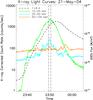 |
Fig. 1 RHESSI corrected count rates between 23:35 and 00:05 UT in various energy ranges (green: 12–25 keV, cyan: 25–50 keV, orange: 50–100 keV) and GOES flux between 1.0 and 8.0 Å (dashed line). The vertical dash-dotted lines at 23:49:30 and 23:50:30 UT indicate the time interval used for imaging spectroscopy. |
The aim of this paper is to study trapping of energetic electrons in two distinct energy domains. For that purpose, we used the analysis of Kuznetsov & Kontar (2015) of radio-emitting energetic electrons above a few hundred of keV, and we analyzed X-ray emission of energetic electrons with energies below 100 keV. We therefore show in this paper that the scattering mean free path of electrons decreases with increasing electron energy. Sect. 2 presents the imaging spectroscopy of the 2007 May 21 flare in X-rays. The spatial and spectral distributions derived from the X-ray observations are presented in Sect. 3. The interpretation of X-ray observations, comparison between X-ray and radio observations, and comparison with the predictions of the diffusive transport model of Kontar et al. (2014) are discussed in Sect. 4, along with the energy dependence of the scattering mean free path of energetic electrons in the frame of that model. Alternative mechanisms and improvement of the diffusive transport models are discussed in Sect. 5. The main results are summarized in Sect. 6.
2. X-ray imaging spectroscopy at the peak of the flare
The M2.6 flare on 2004 May 21 flare, in active region 10618, was detected by RHESSI in the 3–100 keV range. The RHESSI corrected count rates at relevant energies bins are presented on Fig. 1, together with the X-ray flux from GOES. In this figure the count rates are corrected from the changes of the attenuator and decimation states. The peak of the RHESSI count rates is around 23:50 UT, which is about 2 min before the GOES X-ray peak. In Fig. 1, the vertical dash-dotted lines show the time interval (23:49:30 to 23:50:30 UT) chosen to image the X-ray emitting sources. We chose the time interval with the highest signal above 25 keV. A consequent peak in the 25–100 keV light curve is visible between 23:56:00 and 23:58:30 UT, but it was not possible to reconstruct a reliable image above 25 keV during this time interval. The photon statistic is also too low to enable reliable imaging spectroscopy on other one-minute intervals after the X-ray peak of the flare because of the high level of noise in the images, and therefore, the time evolution of X-ray emission is not discussed in this paper.
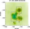 |
Fig. 2 CLEAN image (beam factor 1.7) between 23:49:30 and 23:50:30 UT at 25–50 keV. Contours are 30%, 50%, 70%, and 90% of CLEAN images at 10–25 keV (blue), 25–50 keV (green), and 50–100 keV (orange). Boxes 0, 1, 2 are used for imaging spectroscopy of the looptop source, the first footpoint, and the second footpoint, respectively. |
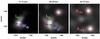 |
Fig. 3 RHESSI images in 3 of the 20 energy bins used for imaging spectroscopy, integrated between 23:49:30 and 23:50:30 UT with 50% of the maximum value encircled in red. Source lengths and widths are shown with green and blue arrows, respectively. At 10–12 keV, the X-ray emission is thermal and we therefore show the length and width of the thermal source Lth and Wth. At 26–28 keV, the emission is non-thermal and we therefore show the length and width of the non-thermal looptop source LLT and WLT. At 60–75 keV, the area of the footpoint sources is calculated with the 50% contour in red. |
2.1. X-ray imaging of the source
Image and contours at 12–25, 25–50, and 50–100 keV are presented in Fig. 2. The geometry of the source can be interpreted as a single loop structure with two footpoints. A coronal hard-X-ray source is visible on the top of the loop structure at 12–25 and 25–50 keV, and the two footpoints are visible in the 25–50 and 50–100 keV ranges. The loop was divided in three regions (see Fig. 2) in order to perform imaging spectroscopy on the looptop source and the two footpoints. The image reconstruction was carried out over a 60 s time interval during the main hard X-ray peak, between 23:49:30 and 23:50:30 UT, using the CLEAN algorithm (Hurford et al. 2002) with a beam factor value of 1.7. The beam factor was carefully chosen as it has an important impact on the determination of the source sizes (see Sect. 2.3 and Appendix A). All collimators except the first one (with the smallest pitch) were used, achieving a spatial resolution of 3.9 arcsec.
To carry out imaging spectroscopy, we reconstructed CLEAN images in 20 narrow energy bins between 10 and 100 keV with increasing width of the bins with energy; that is, 2 keV width between 10 and 30 keV, 3 keV width between 30 and 45 keV, 5 keV width between 45 and 60 keV, 15 keV bin between 60 and 75 keV, and 25 keV bin between 75 and 100 keV. Three images over the 20 images produced are presented in Fig. 3 with 50% contours in red. On these images, the looptop source is visible between 10 and 36 keV and the footpoints are visible above 28 keV. The visibility of looptop and footpoint sources in the images is of course limited by the dynamic range of the images.
Values of free spectral parameters obtained for looptop source and for first and second footpoints.
2.2. Spectral analysis
Each of the 20 images reconstructed between 10 and 100 keV contributes to a single point in the spectrum. The spectra of each region defined in Fig. 2 were fitted using a combination of a thermal and a non-thermal components in OSPEX (Schwartz et al. 2002). The three spectra resulting from the fits are shown in Fig. 4 and the values of the free parameters are described in Table 1.
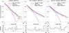 |
Fig. 4 Count flux spectra (data and fit) with residuals for looptop source (left), first footpoint (middle), and second footpoints (right), as defined by the black boxes in Fig. 2. The spectra derived from the data are shown in black. The blue curve represents the thermal component of the fit and the green curve represents the non-thermal component. The pink dash-dotted line represents the component due to albedo correction. The red curve indicates the total fitted spectrum. |
The thermal model has two free parameters that are adjusted during the fit: the temperature and emission measure of the X-ray emitting plasma. The non-thermal part of the spectra was fitted with two different models computing the X-ray flux from a single power-law distribution of energetic electrons. In the looptop source (region 0 in Fig. 2), we assume for simplicity that energetic electrons lose only a small portion of their energy through collisions and that the region can be considered as a thin target. The free parameters of the thin target model are the electronic spectral index δLT and a normalization factor 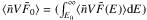 (electrons s-1 cm-2), where
  is the mean density of the thin target, V is its volume, and
  is the energetic electron mean spectrum in electrons s-1 cm-2 keV-1 (see Eq. (B.6)in Appendix B). In the footpoints (regions 1 and 2 in Fig. 2), the density is much higher and energetic electrons instantaneously lose all their energy in the target, which is considered as a thick target. The free parameters of the thick target model are the electronic spectral index δFP and the electron rate above E0, Ṅ (electrons s-1), entering the target (see Eq. (B.15)in Appendix B). In each case, a minimum correction for albedo was used, assuming an isotropic beam of electrons. The low energy cutoff of the non-thermal model, E0, of the non-thermal model (thick or thin target models) was fixed to 25 keV because when this parameter was set free in the spectral analysis, it reached 23 keV.
2.3. Sizes and density of the thermal and non-thermal X-ray sources
In the further calculation of the electron rate for various X-ray sources (see Sect. 3.1), we needed to estimate the sizes of the X-ray emitting regions: the coronal source and the footpoints. Moreover, we distinguished the thermal X-ray emitting region from the non-thermal X-ray emitting region in the coronal source. We used 50% CLEAN contours from the images to estimate the length, width, or area of the X-ray sources. The CLEAN images were produced with a beam factor of 1.7. The determination and influence of this parameter are discussed in Appendix A.
The size of the thermal coronal source was measured at 10–12 keV to ensure the X-ray emission is entirely thermal (see the looptop spectrum in the left panel of Fig. 4). The size of the non-thermal X-ray source at the looptop was measured at 26–28 keV, since at this energy, the looptop source is still visible in the image and the X-ray spectra is predominantly non-thermal (see the looptop spectrum in the left panel of Fig. 4). Finally, the area of the footpoints is taken at 60–75 keV. The measurements of the length and width of the coronal sources are represented by green and blue arrows, respectively, in Fig. 3 and schematically explained in Fig. 5. The measured sizes and areas are summarized in Table 2.
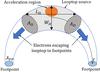 |
Fig. 5 Sketch of a symmetrical magnetic loop. The limits of the looptop sources are the cross sections of the loop with area ALT shown in gray. The length LLT and width WLT of the looptop X-ray source are used to determine the size of the looptop source, which is approximated to a cylinder of diameter WLT. Blue arrows represent the electron rate for electrons leaving the looptop source of cross-section ALT. |
The emission measure EM, given by the spectral analysis (see Table 1) of the thermal part of the coronal source and the estimation of the size of the thermal source (see Table 2), leads to the following estimation of the density: 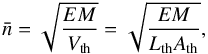 (1)where is the density (in cm-3) and Vth is the volume of the thermal source (in cm3). The values Lth, Wth, and Ath are the length, width, and cross section of the thermal source, respectively, where
  . The assumed geometry of the loop is described in Fig. 5.
The mean plasma density obtained is 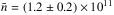 cm-3. This value is in the range of densities calculated by Simões & Kontar (2013) for events in which a non-thermal looptop source is visible.
3. Determination of spatial and spectral distributions of X-ray emitting energetic electrons
3.1. Comparison of electron rates
As explained below, the electron rate above E0 = 25 keV of electrons leaving the looptop source was found to be about ṄLT = (0.4 ± 0.2) × 1035 electrons s-1.
Indeed, the electron rate ṄLT (in electrons s-1) in the looptop source is given by 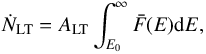 (2)where E0 is the low energy cutoff (in keV), ALT (cm2) is the cross section of the looptop source, assuming a symmetrical source, as shown in Fig. 5; and is the mean energetic electron spectrum in electrons s-1 cm-2 keV-1. We assume energetic electrons propagating in both directions along the loop axis (see the blue arrows in Fig. 5).
For a source with an homogeneous ambient plasma, we can express the looptop electron rate as follows: 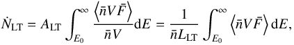 (3)where
 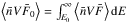 is given by the spectral analysis of the looptop source (see Table 1) and LLT is measured based on the 26–28 keV CLEAN image (see Table 2).
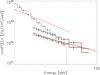 |
Fig. 6 Spatially integrated and density weighted mean flux spectra for looptop (dashed line) and footpoint sources (plain lines) deduced from X-ray observations (black histograms), and computed with the diffusive transport of Kontar et al. (2014) model with n = 9.5 × 1010 cm-3, d = 5.5 Mm, and λ = 1.4 × 108 cm (red). The dotted vertical line indicates the energy at which the coronal and second footpoint spectra cross. |
We compared the electron rate obtained for the looptop source, ṄLT = (0.4 ± 0.2) × 1035 electrons s-1, to the electrons rates obtained by the spectral analysis of the two footpoints, which are (0.12 ± 0.03) × 1035 and (0.06 ± 0.02) × 1035 electrons s-1. The sum of the rates from the footpoints is therefore significantly lower than the rate needed to explain the non-thermal emission in the coronal source; the ratio  is about 2.2 for this event for electrons above E0 = 25 keV.
3.2. Spatial and spectral distributions of mean flux spectrum and density of energetic electrons
Using Eqs. (B.6)and (B.15)(in Appendix B) and the results of the spectral analysis listed in Table 1, the spatially integrated density weighted mean flux spectra ⟨nVF(E)⟩ of the looptop source and footpoints are plotted in Fig. 6 in black. In this figure, the energies for which the footpoint spectra are crossing the looptop spectrum are 50 keV and 60 keV for the first and second footpoints, respectively.
The spatial distribution of energetic electrons ⟨nVF⟩ at 25 keV is also known in three locations in the loop, i.e., the looptop and footpoints. The distance between the footpoints and looptop source was estimated by taking the distance between the centers of the boxes defined in Fig. 2. Kuznetsov & Kontar (2015) showed that the maximum of the spatial distribution of energetic electrons was shifted of 3.2 Mm in regards to the top of the magnetic loop. This three-point distribution is shown in Fig. 7.
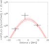 |
Fig. 7 Spatial distribution of energetic electrons at 25 keV deduced from X-ray observations (black crosses) and computed with the diffusive transport model of Kontar et al. (2014) with n = 9.5 × 1010 cm-3, d = 5.5 Mm and λ = 1.4 × 108 cm (red lines). The looptop source is shifted of 3.2 Mm in regards to the top of the loop, as described in Kuznetsov & Kontar (2015). For the model, the dashed or dotted lines indicate a confidence interval around the computed value shown by the plain line. A detailed description is provided in Sect. 4.1. |
The number density of energetic electrons with energy E>Emin,  (in electrons cm-3), is defined as
 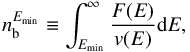 (4)where v is the velocity of the electrons. In the following, we distinguish the estimation of in the thin and thick target models. The details of the calculations are in Appendix B.
Using Eqs. (B.7)and (B.16)with Emin = E0 = 25 keV, we can evaluate the electron density of energetic electrons with energy E> 25 keV,  in the thin and thick target models, respectively. We found
 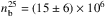 electrons cm-3 in the corona and
 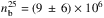 and (4 ± 3) × 106 electrons cm-3 in each footpoint. We estimated of the area of the cross section of the loop ALT to calculate the number density of energetic electrons from the observations. From the size estimation shown in Table 2, we found
  Mm2. The spatial distribution of the energetic electron density above 25 keV electrons in the flaring loop is plotted on Fig. 8.
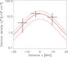 |
Fig. 8 Spatial distribution of density of energetic electrons with energy E> 25 keV deduced from observations ( |
Summary of the influence of density n, size of the acceleration region d, and scattering mean free path λ on spatial and spectral distributions of energetic electrons in the frame of the diffusive transport model.
4. Interpretation of the observations in the context of diffusive transport of energetic electrons
4.1. Confinement of X-ray producing energetic electrons
The spectral indexes of the electron distribution from the X-ray emission, using the thin and thick target models are summarized in Table 1. While electron spectral indexes in both footpoints are very close and are considered as similar, the electron spectral index in the looptop source is softer by ≈ 1. Furthermore, the ratio of the electron rate in the looptop source and footpoints is found to be around 2.2. These values are similar to values found for other events (see, e.g., Simões & Kontar 2013). These results suggest that a significant number of high energy electrons are confined in the coronal region. Such a confinement of high energy electrons can result from magnetic mirroring or turbulent pitch-angle scattering as demonstrated in Kontar et al. (2014), Bian et al. (2011). In the following, we investigate whether the confinement observed in this flare can be explained in the context of the diffusive transport model of Kontar et al. (2014). In this model, strong, turbulent pitch-angle scattering due to small-scale fluctuations of the magnetic field, is responsible for a diffusive parallel transport of energetic particles and finally results in a confinement mechanism.
4.1.1. Effects of the diffusive transport on energetic electron distributions
In Sect. 4.1.2 we compared the observed spatial and spectral distributions of ⟨nVF⟩ with those calculated in the diffusive transport model described in Kontar et al. (2014). The distribution FD(E,z) (electrons/cm2/s/keV) of energetic electrons of energy E at a position z along the magnetic loop is indeed described by the following equation (Kontar et al. 2014): ![Mathematical equation: \begin{eqnarray} F_D(E,z) &=& \frac{E}{Kn}\int_E^{\infty} {\rm d}E' \frac{F_0(E')}{\sqrt{4a\pi(E'^2-E^2)+2d^2}} \notag\\[1.5mm] &&\quad \times \exp{\left(\frac{-z^2}{4a(E'^2-E^2)+ 2d^2}\right)}, \label{equation} \end{eqnarray}](/articles/aa/full_html/2018/02/aa31514-17/aa31514-17-eq98.png) (5)where F0(E) is the initial distribution of energetic electrons in the source (acceleration) region supposed to be spatially extended, d is the size of the acceleration region (Gaussian form), n is the plasma ambient density, K = 2πe4Λ is the collisional parameter, and a = λ/ (6Kn), where λ is the pitch-angle scattering mean free path of the electrons. In the work of Kontar et al. (2014), this mean free path λ is considered to be independent of energy.
(5)where F0(E) is the initial distribution of energetic electrons in the source (acceleration) region supposed to be spatially extended, d is the size of the acceleration region (Gaussian form), n is the plasma ambient density, K = 2πe4Λ is the collisional parameter, and a = λ/ (6Kn), where λ is the pitch-angle scattering mean free path of the electrons. In the work of Kontar et al. (2014), this mean free path λ is considered to be independent of energy.
In Eq. (5)the plasma density n, the size of the acceleration region d and the scattering mean free path of electrons λ are parameters of the model. The effects of these parameters on both spatial and spectral distributions of energetic electrons is shown in Fig. 10 and summarized in Table 3. The spectral indexes obtained in the corona and footpoints for each set of parameters are described in Table 4.
Influence of density n, size of acceleration region d, and scattering mean free path λ on spectral index of non-thermal electron distributions in the frame of the diffusive transport model.
As shown in Fig. 10, the different parameters do not influence the two distributions in the same way. For instance, when d or λ increases, the spatial distribution becomes broader, but the shape of the distribution remains different. Moreover, the effects on the spectra are not the same: increasing d has almost no impact on the coronal spectrum, whereas increasing λ leads to a softening of the coronal spectrum.
It can be seen that the increase of density leads to an enhanced trapping of energetic electrons, even if the scattering mean free path remains unchanged.
In addition, there is a limit to the value of the size of the acceleration region below which the effect of this parameter is negligible; this is the case when d2 ≪ aπ(E′2−E2) (see Eq. (5)). In our conditions, the influence of d on the energetic electron distributions is negligible for d ≲ 108 cm.
4.1.2. Model fitting to the observed energetic electron distributions
In the following, the electron distribution in the looptop and footpoints were computed through integration of Eq. (5) on z from − 7 Mm to 5 Mm for looptop sources and from − 9 Mm to − ∞ and from +13 Mm to + ∞ for footpoint sources, respectively. We needed to determine the injected distribution of electrons F0 and make the parameters n, d, and λ vary to fit the distributions derived from these equations to the observations. As discussed in Kontar et al. (2014) and also shown in Sect. 4.1.1, the increase of diffusion due to pitch-angle scattering results in enhanced coronal emission and weaker footpoint emission than in the standard nondiffusive case owing to the increase of the time spent by the electrons in the corona. In the diffusive case, the spectrum of the electrons in the corona becomes progressively flatter and the scattering mean free path decreases. However, as shown in Sect. 4.1.1, the mean electron spectrum in the footpoint is less affected by the increase of diffusion than the electron spectrum in the corona. This is why in the remainder of the paper, we assume that the injection spectrum of the energetic electrons is given by the spectral index of the population of the electrons entering the footpoints. The injected electron rate cannot be directly inferred from the results of the spectral analysis of the observations. Indeed, the value found in the footpoints is too low because there are trapped electrons while the electron rate computed in the corona (see Sect. 3.1) is too high since there are some trapping effects. Therefore, the injected electron rate is considered as a free parameter to fit the model to the observations with the constraint that its value Ṅi must be between the two boundaries ṄFP and ṄLT. This parameter has no effect on the spatial distribution of energetic electrons but impacts the normalization of the spatial distribution of the density of energetic electrons.
Once the initial distribution of electrons is determined, the spatial and spectral distributions of energetic electrons in the coronal source and footpoints depends on the density of the ambient medium n, size of the acceleration region d, and the scattering mean free path of electrons λ (see Eq. (5)). We searched for the best set of parameters that could reproduce, at the same time, the spatial distribution of energetic electrons at 25 keV and the spectral distribution of energetic electrons in the footpoints (Figs. 6 and 7). As described in Sect. 4.1.1, each parameter affects both spatial and spectral distributions. A major effect was found for the width of the spatial distribution and the slope of the electron spectrum in the corona. The space of four parameters (Ṅ, n, λ, and d) was explored by producing predicted spatial and spectral distributions of energetic electrons that could be compared to those deduced from X-ray observations. A χ2 was computed for each set of parameter, as described in Appendix C. The minimal χ2 was found for the following set of parameters:  s-1,
s-1,  cm-3,
cm-3,  cm, and
  cm. The uncertainties on the parameters represent the values for which the χ2 exceed the minimal χ2 by at least 5% (see Appendix C). The modeled distributions are plotted in Figs. 6 and 7. We can note that the slope of the looptop spectra is not well recovered by the model. On the other hand, the modeled spatial distribution does not seem to be as peaked that expected from the data. This is a consequence of a trade off that happens during the fit to both spatial and spectral distributions. Nevertheless, the models fit the data with a density close to the density deduced from the observations and an electron injection rate close to the electron rate deduced in the looptop source.
The spatial distribution of the energetic electron density is also computed with the set of parameters found above and compared with the values derived from the fit of the observations (see Fig. 8). The cross section of the loop ALT was fixed to 26 Mm2 as this area was used to calculate the electron density from the observations. In the different plots, the estimation of the error on the values of δthick and ṄLT is taken into account and is responsible for the error intervals around the distributions derived from the model and is visible in Figs. 7–9.
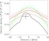 |
Fig. 9 Spatial distribution of density of energetic electrons with energy E> 60 keV, at looptop, estimated from X-ray observations ( |
4.2. Comparison of radio observations with model predictions
The 2004 May 21 flare gyrosynchrotron emission has been studied by Kuznetsov & Kontar (2015). The gyrosynchrotron emission is produced mostly by electrons of energies around 400 keV, and therefore the radio observations of the flare have allowed us to study energetic electrons in a different energy domain than the X-ray analysis because X-ray emitting electrons are mostly in the 25–100 keV energy range.
4.2.1. Comparison between X-ray and radio observations
The spatial distributions of electrons at 25 keV (Fig. 7) and of the density of energetic electrons in the loop (Fig. 8) show that most of the energetic electrons with energy E> 25 keV are located in the looptop source. Moreover, an asymmetry is seen between the two footpoints. Both results are in agreement with the results obtained by Kuznetsov & Kontar (2015) who calculated the spatial distribution of the density of energetic electrons with energy E> 60 keV ( ) from observations of the gyrosynchrotron emission (see Fig. 7 in Kuznetsov & Kontar 2015, and Fig. 9 in the present paper). To compare with the results of Kuznetsov & Kontar (2015), we estimated the number density of energetic electrons above 60 keV from the X-ray observations, using the relation
 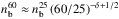 with δ = 4.2:
  electrons cm-3 in the corona. This estimate of from X-ray producing electrons at the looptop is plotted as a cross in Fig. 9. It is about two times lower than the value found by Kuznetsov & Kontar (2015) from radio observations (see Fig. 9). This difference could be explained if there is a break in the power-law spectrum of the energetic electrons with a smaller spectral index at higher energy or if the thin target approximation in the coronal source must be relaxed as suggested by the flatter spectrum of electrons in the coronal source derived in the model.
Independent of this quantitative comparison of relative numbers of electrons producing X-rays and radio emissions, we compared the relative spatial distributions of both X-ray-emitting electrons and radio-emitting electrons by comparing the ratio between the maximum electron density in the loop and the number density in the footpoints. The ratios between the number densities of energetic electrons at the looptop and footpoints,  , from the X-ray measurements, are 1.6 and 3.8 for the first and second footpoint, respectively. Taking the values at the same distance in Fig. 7 in Kuznetsov & Kontar (2015), the ratios
  , averaged over the three times, are 7.7 and 9. The ratio is much higher for the distribution deduced at energies above 60 keV from the gyrosynchrotron emission than for that deduced at 25 keV from HXR observations. This implies that the X-ray-emitting energetic electron spatial distribution is less strongly peaked than the spatial distribution deduced from microwave emissions, as seen in Fig. 9, and that the high energy electrons responsible for gyrosynchrotron emissions are more confined in the corona than the lower energy electrons. Based on the discussion in Sect. 4.1.1 and assuming that X-ray and radio emissions are produced by the same electrons injected and confined in the same loop (the values of d and n remain unchanged), the only way to produce a more spatially peaked distribution is to vary the scattering mean free path λ. Therefore, a second fit was performed on the distribution of the density of energetic electrons deduced from radio observations, where the only free parameter is the scattering mean free path λ. The ambient density and size of the acceleration region are kept as they were found by fitting the distributions deduced from X-ray observations. Figure 9 shows the modeled distribution with
  cm, which produced the smallest χ2. Details of the fit are described in Appendix C.
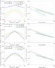 |
Fig. 10 Influence of free parameters in Eq. (5)(n the plasma density, d the size of the acceleration region, and λ the scattering mean free path) on the spatial (left panels) and spectral (right panels) distributions of energetic electrons. In the top panels, d and λ are constant and n = 5 × 109 cm-3 (blue), n = 4 × 1010 cm-3 (green), and n = 1011 cm-3 (orange). In the middle panels, n and λ are constant and d = 2 × 108 cm (blue), d = 6 × 108 cm (green), and d = 12 × 108 cm (orange). In the bottom panels, n and d are constant and λ = 108 cm (blue), λ = 3 × 108 cm (green), and λ = 109 cm (orange). The dotted vertical lines indicate the energies at which the coronal spectrum crosses the footpoint spectrum. |
5. Discussion
In this paper, we focused on the interpretation of our observations in the frame of the diffusive transport model described in Kontar et al. (2014). We showed that the diffusive transport model of Kontar et al. (2014) can explain the observed trapping of energetic electrons in the corona. In particular, the model explains the electron spectrum in the footpoint, the hardening of the footpoint spectrum compared to the coronal spectrum, and the spatial distribution of energetic electrons along the loop. However, diffusive transport of energetic electrons is not the only mechanism that can explain electron trapping in the corona and we include a discussion about trapping with magnetic mirrors at the end of this section.
5.1. Comparison with scattering mean free path in the interplanetary medium
The spatial distributions of X-ray emitting and radio emitting electrons can be reproduced in the context of the diffusive transport model of Kontar et al. (2014) only by assuming that the scattering mean free path of energetic electrons decreases with increasing electron energy, which explains why the trapping of energetic electrons in the corona is stronger at higher energies. This conclusion is of course contradictory to the assumption of the model in which the scattering mean free path is constant with energy and shows that to study the behavior of X-ray and radio emissions completely, a new model should be developed in which the scattering mean free path depends on energy. This is however, out of the scope of the present paper. We shall however discuss the result on the energy dependance of the scattering mean free path with respect with what is observed in the interplanetary medium. Several studies (see, e.g., Dröge 2000b; Agueda et al. 2014) have found for interplanetary electrons in range 0.1–1 MV a power-law dependence of the electron mean free path on rigidity with a negative power-law index. We therefore also assume a power-law dependence of the electron scattering mean free path with energy in the present study. We have only two data points; the first is derived from X-ray radiation above 25 keV and the second is derived from radio observation, which is produced mostly by electrons at 400 ± 100 keV (priv. commun. from A. Kuznetsov). The mean free paths calculated in this paper are plotted as a function of electron energy in Fig. 11. Given the uncertainty about the energy of radio-emitting electrons, and the uncertainty on the mean free path, we can calculate the slope of the power law in two limit cases, − 1.9 and − 0.3. The corresponding slopes for the mean free path dependence in rigidity are between − 3.4 and − 0.5. Although it is clear that the scattering mean free path is decreasing with increasing electron energy and rigidity, a large range of slopes are consistent with our data. It should be pointed out that, five out of seven events studied by Agueda et al. (2014) have shown slopes for the rigidity dependence of the scattering mean free path of electrons in the interplanetary medium that could be consistent with our observations.
5.2. Limitations and future improvements to the diffusive transport model
The diffusive transport model predictions did not perfectly reproduce the observations in the detail. In particular, the predicted looptop source spectrum is flatter than the spectrum deduced from the X-ray analysis of the flare. This difference could be because some effects are not taken into account in the diffusive transport equation that has been used in this paper, such as the effect of a converging magnetic field. This discrepancy can also be explained by the fact that the thin target approximation might not be valid for the coronal source in this context. Indeed, the density calculated in the coronal source (1.2 ± 1011 cm-3) is a little high and the source could be considered as a thick target for low energy electrons. Moreover, the diffusion of energetic electrons in the corona leads to enhanced time spent by the electrons in the target, where they lose more energy than assumed in the thin target approximation. However, assuming that the coronal X-ray source is a thick target in the spectral analysis does not improve the agreement between the data and the predictions of the diffusive transport model. The X-ray coronal source is most probably neither a thick nor thin target, but is in between, with a density where neither of these two approximations are completely valid. Finally, the normalization of the modeled distribution of the density of energetic electrons above 60 keV is not well recovered. This might indicate that fewer energetic electrons than expected are accelerated at energies above 60 keV (e.g., the injection electron rate decreases with energy), but it most probably because the model produces a coronal spectrum that is too flat and therefore overestimates the number of high energy electrons in the loop.
We show that the diffusive transport can explain the observed spatial and spectral distributions in the X-ray and radio ranges if the mean free path is energy dependent. The mean free path has been assumed to be constant in Kontar et al. (2014). A further development of this model should include the energy dependence of the mean free path and the relativistic effects to allow a more precise comparison of the model prediction with combined X-ray and radio observations.
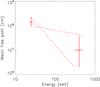 |
Fig. 11 Energy dependence of scattering mean free path calculated with the diffusive transport model of Kontar et al. (2014), where ALT = 26 Mm2, d = 5.5 Mm, n = 9.5 × 1010 cm-3. The uncertainties on the values of the mean free path derived from the fit (see Appendix C) and on the energy of the radio-emitting electrons are taken into account. The two most extreme slopes for the power-law dependence of the mean free path are plotted. |
5.3. Trapping with magnetic mirrors
Trapping of energetic electrons in the coronal part of the loop can be explained by the effect of a converging magnetic field. In this event, the area of the section of the loop calculated (26 Mm2) at the ends of the coronal source is larger than the area of the footpoints deduced from X-ray observations (see Table 2); this observation is in favor of a magnetic convergence of the loop. If we consider a magnetic loss cone for the electron pitch-angle distribution, the loss-cone angle α0 depends on the magnetic ratio σ, as described in the introduction. The trapped fraction of the energetic electron distribution is deduced from X-ray observations and is  (see Simões & Kontar 2013, for more details). Simões & Kontar (2013) showed that in the case of an isotropic pitch-angle distribution, the trapped fraction of the energetic electron distribution is equal to μ0, the cosine of the loss-cone angle α0. We can therefore retrieve the value of σ needed to explain the observed ratio in the case of an isotropic pitch-angle distribution; we found σ ≈ 1.4, which is close to the values found by Simões & Kontar (2013), Aschwanden et al. (1999b), Tomczak & Ciborski (2007) and explains the observed ratio of cross sections of the loop at the looptop and in the footpoints. This expected value σ of the magnetic ratio can be compared to the magnetic ratio measured in the loop σr.
To estimate the magnetic ratio σr of the coronal loop, we can use the magnetic extrapolation from Kuznetsov & Kontar (2015). In doing so, we assume that the HXR and gyrosynchrotron emissions are produced in a same magnetic loop, as mentioned in the introduction. As it can be seen in Fig. 6 in Kuznetsov & Kontar (2015), at the looptop of the reconstructed magnetic loop, the magnetic field strength is BLT ≈ 360 G.
Using the estimation of the source length seen in X-ray, we determined the value of the magnetic field at the supposed position of the mirrors (at each end of the observed coronal X-ray source) and found values of 430 ± 30 and 570 ± 30 G, leading to the following values of the magetic ratio: σr ≈ 1.2 and 1.6. This is consistent with the ratios of loop cross sections at the looptop and footpoints that are deduced from the X-ray images, which are ≈ 1.4 and 1.5 for the two footpoints. The magnetic ratio measured is therefore just enough to explain the ratio of electron rate deduced from the X-ray observations. However, with this model, it is a priori not possible to explain why the trapping of energetic electrons is stronger at higher energies and why a spectral hardening with a difference of 1 between electronic spectral slopes is observed between the looptop and footpoint sources. Also, Kuznetsov & Kontar (2015) showed a shift between the centroid of the gyrosynchroton source and the top of the magnetic loop where the magnetic field is minimal. In the case of electron trapping due to magnetic mirroring, we expect to have a maximum emission where the magnetic field is minimum.
6. Summary and conclusions
The summary of our observations is the following:
-
1.
The difference between the footpoint and looptop spectralindexes is about 1, which suggests that amechanism is hardening the electron spectrum during thetransport. This can be explained by trapping of energeticelectrons in the corona.
-
2.
The ratio of the looptop and footpoint electron rate above 25 keV,
, has a value of 2.2, suggesting that part of the energetic electrons are trapped in the coronal part of the loop. -
3.
The spatial distribution of HXR-emitting electrons is peaked near the looptop, but less peaked than the spatial distribution of microwave-emitting electrons since the ratio of energetic electron density between the looptop and footpoints is more than two times higher for radio-emitting electrons above 60 keV than X-ray emitting electrons above 25 keV.
-
4.
The spectral and spatial distribution of energetic electrons, deduced from both X-ray and radio observations, can be explained by a diffusive transport model of Kontar et al. (2014), with a mean free path decreasing with increasing electron energy.
-
5.
The mean free path for electron energies between 25 and 100 keV is on the order of 1.4 × 108 cm, which is smaller than the length of the loop. These values are comparable to values found by Kontar et al. (2014). The mean free path is also smaller than the size of the acceleration region calculated with the model (5.5 × 108 cm), which suggests that electrons can potentially be accelerated for a longer time.
-
6.
The scattering mean free path for electron energies around 400 keV (107 cm) is significantly smaller than the mean free path estimated at lower energies. Similar dependence of the scattering mean free path over electron energies has been found in the case of interplanetary electron transport in the same range of electron energy. The potential slopes of the energy dependence of the scattering mean free path in the solar corona are in agreement with some of the slopes observed for interplanetary electrons.
Trapping due to magnetic mirroring is not known to be energy dependent and this mechanism cannot fully explain our observations.
The diffusive transport model enable the reproduction of our different observations, such as the spectral slope in the footpoints, some spectral hardening between the looptop and footpoints, and the spatial distributions of electron density deduced from both X-ray and radio observations.
Imaging spectroscopy in HXR is a powerful tool to study electron transport during solar flares. This study should encourage the development of predictions on the spatial distribution of electrons and the evolution of the spectral index of non-thermal electron energy distribution by the various transport models. The simultaneous observation of non-thermal X-ray sources in both the coronal part of the loop and its footpoints is rare because footpoints sources are usually brighter than coronal sources and indirect imaging instruments, such as RHESSI, have a limited dynamic range. Instruments using focusing optics for hard X-ray imaging (such as the FOXSI spacecraft) would therefore provide very useful observations of faint non-thermal coronal sources in the presence of bright footpoints and therefore add interesting cases in which to study electron transport during flares.
Finally, this study shows that the combination of X-ray and radio diagnostics for energetic electrons in closed loops during flare enable us to study the energy dependence of transport properties in the solar corona, such as the scattering mean free path. Such observations could constrain, to some extent, some properties of the turbulence spectrum in the solar corona.
The rigidity R of a charged particle is defined by R = pc/q, where p is the momentum of the particle, q is its charge, and c is the speed of light. For relativistic particles,  , where E is the kinetic energy and m the mass of the particle.
The lower limit adopted in Kuznetsov & Kontar (2015) is 60 keV even if the radio emissivity is maximum for electrons of a few hundred of keV (Kuznetsov, priv. commun.).
Acknowledgments
We thank the RHESSI team for producing free access to data, Alexey Kuznetsov for his help with the radio data, and our referee for his useful comments. Sophie Musset acknowledges the CNES and the LABEX ESEP (N° 2011-LABX-030) for Ph.D. funding, and thanks the French State and the ANR for their support through the “Investissements d’avenir” program in the PSL∗ initiative (convention N° ANR-10-IDEX-0001–02), as well as the Programme National Soleil-Terre (PNST). EPK was supported by a STFC consolidated grant ST/L000741/1.
References
- Agueda, N., Klein, K.-L., Vilmer, N., et al. 2014, A&A, 570, A5 [NASA ADS] [CrossRef] [EDP Sciences] [Google Scholar]
- Arnoldy, R. L., Kane, S. R., & Winckler, J. R. 1968, ApJ, 151, 711 [NASA ADS] [CrossRef] [Google Scholar]
- Aschwanden, M. J., Fletcher, L., Sakao, T., Kosugi, T., & Hudson, H. 1999a, ApJ, 517, 977 [NASA ADS] [CrossRef] [Google Scholar]
- Aschwanden, M. J., Fletcher, L., Sakao, T., Kosugi, T., & Hudson, H. 1999b, ApJ, 517, 977 [NASA ADS] [CrossRef] [Google Scholar]
- Bai, T. 1982, ApJ, 259, 341 [NASA ADS] [CrossRef] [Google Scholar]
- Battaglia, M., & Benz, A. O. 2006, A&A, 456, 751 [NASA ADS] [CrossRef] [EDP Sciences] [Google Scholar]
- Bian, N. H., Kontar, E. P., & MacKinnon, A. L. 2011, A&A, 535, A18 [NASA ADS] [CrossRef] [EDP Sciences] [Google Scholar]
- Bieber, J. W., Matthaeus, W. H., Smith, C. W., et al. 1994, ApJ, 420, 294 [Google Scholar]
- Brown, J. C., Emslie, A. G., & Kontar, E. P. 2003, ApJ, 595, L115 [NASA ADS] [CrossRef] [Google Scholar]
- Dennis, B. R., & Pernak, R. L. 2009, ApJ, 698, 2131 [NASA ADS] [CrossRef] [Google Scholar]
- Dröge, W. 2000a, Space Sci. Rev., 93, 121 [NASA ADS] [CrossRef] [Google Scholar]
- Dröge, W. 2000b, ApJ, 537, 1073 [NASA ADS] [CrossRef] [Google Scholar]
- Emslie, A. G., Kontar, E. P., Krucker, S., & Lin, R. P. 2003, ApJ, 595, L107 [NASA ADS] [CrossRef] [Google Scholar]
- Holman, G. D., Aschwanden, M. J., Aurass, H., et al. 2011, Space Sci. Rev., 159, 107 [NASA ADS] [CrossRef] [Google Scholar]
- Hurford, G. J., Schmahl, E. J., Schwartz, R. A., et al. 2002, Sol. Phys., 210, 61 [NASA ADS] [CrossRef] [Google Scholar]
- Jokipii, J. R. 1966, ApJ, 146, 480 [Google Scholar]
- Kennel, C. F., & Petschek, H. E. 1966, J. Geophys. Res., 71, 1 [NASA ADS] [CrossRef] [Google Scholar]
- Kontar, E. P., Hannah, I. G., Jeffrey, N. L. S., & Battaglia, M. 2010, ApJ, 717, 250 [NASA ADS] [CrossRef] [Google Scholar]
- Kontar, E. P., Brown, J. C., Emslie, A. G., et al. 2011a, Space Sci. Rev., 159, 301 [NASA ADS] [CrossRef] [Google Scholar]
- Kontar, E. P., Hannah, I. G., & Bian, N. H. 2011b, ApJ, 730, L22 [NASA ADS] [CrossRef] [Google Scholar]
- Kontar, E. P., Bian, N. H., Emslie, A. G., & Vilmer, N. 2014, ApJ, 780, 176 [NASA ADS] [CrossRef] [Google Scholar]
- Kovalev, V. A., & Korolev, O. S. 1981, Soviet Ast., 25, 215 [NASA ADS] [Google Scholar]
- Krucker, S., & Lin, R. P. 2002, Sol. Phys., 210, 229 [NASA ADS] [CrossRef] [Google Scholar]
- Kuznetsov, A. A., & Kontar, E. P. 2015, Sol. Phys., 290, 79 [NASA ADS] [CrossRef] [Google Scholar]
- Leach, J., & Petrosian, V. 1981, ApJ, 251, 781 [NASA ADS] [CrossRef] [Google Scholar]
- Lin, R. P., Dennis, B. R., Hurford, G. J., et al. 2002, Sol. Phys., 210, 3 [Google Scholar]
- MacKinnon, A. L. 1991, A&A, 242, 256 [NASA ADS] [Google Scholar]
- McClements, K. G. 1992, A&A, 258, 542 [NASA ADS] [Google Scholar]
- Melrose, D. B., & Brown, J. C. 1976, MNRAS, 176, 15 [NASA ADS] [CrossRef] [Google Scholar]
- Metcalf, T. R., Hudson, H. S., Kosugi, T., Puetter, R. C., & Pina, R. K. 1996, ApJ, 466, 585 [NASA ADS] [CrossRef] [Google Scholar]
- Palmer, I. D. 1982, Rev. Geophys. Space Phys., 20, 335 [Google Scholar]
- Piana, M., Massone, A. M., Hurford, G. J., et al. 2007, ApJ, 665, 846 [Google Scholar]
- Schmahl, E. J., Pernak, R. L., Hurford, G. J., Lee, J., & Bong, S. 2007, Sol. Phys., 240, 241 [NASA ADS] [CrossRef] [Google Scholar]
- Schwartz, R. A., Csillaghy, A., Tolbert, A. K., et al. 2002, Sol. Phys., 210, 165 [NASA ADS] [CrossRef] [Google Scholar]
- Simões, P. J. A., & Kontar, E. P. 2013, A&A, 551, A135 [NASA ADS] [CrossRef] [EDP Sciences] [Google Scholar]
- Siversky, T. V., & Zharkova, V. V. 2009, A&A, 504, 1057 [NASA ADS] [CrossRef] [EDP Sciences] [Google Scholar]
- Sturrock, P. A. 1968, in Structure and Development of Solar Active Regions, ed. K. O. Kiepenheuer, IAU Symp., 35, 471 [NASA ADS] [Google Scholar]
- Sweet, P. A. 1969, ARA&A, 7, 149 [NASA ADS] [CrossRef] [Google Scholar]
- Syrovatskii, S. I., & Shmeleva, O. P. 1972, Soviet Ast., 16, 273 [Google Scholar]
- Takakura, T. 1986, Sol. Phys., 104, 363 [NASA ADS] [CrossRef] [Google Scholar]
- Tomczak, M., & Ciborski, T. 2007, A&A, 461, 315 [NASA ADS] [CrossRef] [EDP Sciences] [Google Scholar]
- Vilmer, N., Trottet, G., & MacKinnon, A. L. 1986, A&A, 156, 64 [NASA ADS] [Google Scholar]
- Xu, Y., Emslie, A. G., & Hurford, G. J. 2008, ApJ, 673, 576 [NASA ADS] [CrossRef] [Google Scholar]
Appendix A: CLEAN beam factor
The CLEAN algorithm is an iterative algorithm based on the assumption that the X-ray image is well represented by a superposition of point sources convolved with the point spread function (PSF) of the instrument (see, e.g., Hurford et al. 2002). The CLEAN algorithm developed for the RHESSI image analysis has one parameter called “beam factor”, which represents the effective resolution of the subcollimators used to reconstruct the image.
The value for the beam factor was chosen to have CLEAN images as close as possible to images reconstructed with the visibility forward fit VISFF (see Schmahl et al. 2007, for the definition of visibilities and Xu et al. 2008, for examples of application) and the PIXON (Metcalf et al. 1996; Hurford et al. 2002) algorithms. This is a standard procedure to ensure that CLEAN agrees with other algorithms for image reconstruction (see, e.g., Dennis & Pernak 2009; Kontar et al. 2010).
The determination of the best value of the beam factor for the image reconstruction has an important impact on the X-ray source size determination on CLEAN images. For example, when using the default value of the beam factor 1, the measured sizes are roughly 1.5 times greater than the sizes estimated on CLEAN images with a beam factor of 1.7 or on a PIXON image.
Appendix B: X-ray production in thin and thick targets
The bremsstrahlung photon flux at energy ϵ, I(ϵ), produced by an energetic electron flux density distribution F(E,r) (electrons cm-2 s-1 keV-1) in an emitting source (a target) of plasma density n and volume V is expressed as  (B.1)where Q(ϵ,E) is the differential bremsstrahlung cross section, and the integration is done over the target volume and all contributing electron energies, which are all electron energies above the photon energy ϵ.
We can see that the X-ray spectrum I(ϵ) is linked to both the energetic electron distribution and the ambient plasma properties (density and volume of the target).
For spectral observations, we use a spatially integrated form of Eq. (B.1) (B.2)where
  and (electrons cm-2 s-1 keV-1) is the mean electron flux distribution, i.e., the electron flux density distribution that is plasma density weighted and target averaged (Brown et al. 2003; Kontar et al. 2011a; Holman et al. 2011), which is defined as
  (B.3)Since the quantity
  is dimensionless, the units of
  are the same as those of the electron flux (electrons cm-2 s-1 keV-1). The value
  is a quantity that can be retrieved from the X-ray spectrum I(ϵ) without any model assumption and, therefore, is the quantity derived during spectroscopic diagnosics of the X-ray emission. To retrieve the product
  , in principle, we only need to know the bremsstrahlung cross-section Q(ϵ,E).
In our study, we were particularly interested by the number density of energetic electrons with energy E>Emin, (in electrons cm-3), which is defined as 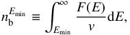 (B.4)where v is the velocity of the electrons. It can also be expressed as
 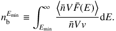 (B.5)We distinguish two approximations, the thin target and thick target models. In the thin target model, energetic electrons lose only a small fraction of their energy while they pass through the target, whereas in the thick target model, energetic electrons lose all their supra-thermal energy in the target.
In the following, we describe how the product  is expressed in the thin and thick target models in OSPEX and how we estimate the energetic electron number density nb (cm-3).
Appendix B.1: Thin target model
We assume a power-law distribution for the electron mean spectrum:  . In OSPEX, the proportionality constant is defined such that we can write the spatially integrated density weighted mean flux spectrum
  (in electrons s-1 cm-2 keV-1) as
 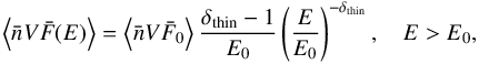 (B.6)where δthin and
 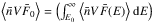 are the spectral index and normalization factor given by the spectral analysis (see Table 1).
Equation (B.5)and can be integrated over E, using Eq. (B.6)to obtain  (B.7)where m is the electron mass (in keV/c2).
Appendix B.2: Thick target model
In the thick target model, energetic electrons lose all their supra-thermal energy through efficient collisions. Therefore, the energetic electron spectrum  is different from the injected electrons spectrum F0. In fact, we need to integrate the injection spectrum over all energies in the X-ray emitting source.
 |
Fig. C.1 Evolution of values of χ2 with free parameters in the model. Left: evolution of χ2 with ambient density n with λ = 1.4 × 108 cm and d = 5.5 Mm. Middle: evolution of χ2 with the size of the acceleration region d with λ = 1.4 × 108 cm and n = 9.5 × 1010 cm-3. Right: evolution of χ2 with the scattering mean free path with d = 5.5 Mm and n = 9.5 × 1010 cm-3. The horizontal line indicates the limit of 5% of the minimal χ2 value that has been used to determine uncertainties on the best values for the model free parameters. |
Therefore, the number of photons of energy between ϵ and ϵ + δϵ produced by an electron of initial energy E0 is  (B.8)where tF is the time at which all energetic electrons have been thermalized. Since energetic electrons are losing energy at a rate dE/ dt, the time integration can be replaced by an integration over energy, i.e.,
  (B.9)Energetic electrons lose their energy by Coulomb collisions with the electrons of the ambient plasma, and in that case the energy loss rate is expressed as
  (B.10)where K = 2πe4Λ, with Λ is the Coulomb logarithm, e is the electron charge, n the density of the plasma, and v is the speed of the energetic electron.
If we consider the injected electron spectrum F0(E0), the X-ray spectrum can be express as 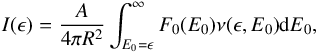 (B.11)where A is the area of the thick target source.
Using Eq. (B.10)in Eq. (B.9), we can rewrite Eq. (B.11)in the following way: 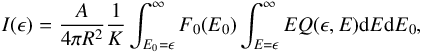 (B.12)and by changing the integration order, and comparing with Eq. (B.2),
 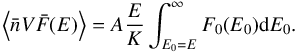 (B.13)Once again, we assume the injection spectrum to have a power-law dependence in energy,
  . In OSPEX, the injection spectrum F0(E) (electrons s-1 cm-2 keV-1) has the following form:
 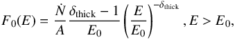 (B.14)where Ṅ is the injection electron rate (in electrons s-1) and δFP is the spectral index.
After integration of Eq. (B.13), the spatially integrated density weighted mean flux spectrum is written as 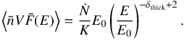 (B.15)
Equation (B.5)is also valid for the thick target model. Using Eq. (B.15)and after integration, the density of energetic electrons, in electrons/cm3, in the thick target, is written as 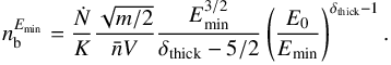 (B.16)
Appendix C: Model fitting
The first fit of the model to the data was performed using the X-ray observations. The electron mean spectra for the coronal source and one footpoint, as well as the spatial distribution of electrons at 25 keV, are modeled and compared to the same distributions deduced from the X-ray observations. These distributions are shown in Figs. 6 and 7. The χ2 is calculated by comparing the looptop spectra between 22 keV and 39 keV, where the observed spectra are mostly non-thermal; by comparing the footpoint spectra between 24 and 100 keV; and by comparing the spatial distribution at the three data points deduced from the observations. The errors on the observations are derived from the errors found on the free parameters in the spectral analysis (see Table 1).
The evolution of the χ2 in regards to the free parameters (n, λ, and d) is shown in Fig. C.1. To provide uncertainties on the values of those parameters, we looked at the values for which the χ2 was 5% larger than its minimum. The resulting density is between 7 × 10¹⁰ and 1.6 × 1011 cm-3, the size of the acceleration region is between 5 and 6.2 Mm, and the scattering mean free path is between 1 × 10⁸ and 2.2 × 108 cm.
The final value of the χ2 is high, which in particular is because the spectral slope of the coronal spectrum is not well recovered.
The fit of the model to the spatial distribution of the density of energetic electrons above 60 keV deduced from radio observations was performed by comparing the modeled distributions on artificially created data points between − 17 and +17 Mm, spaced 0.5 Mm each. The error on the distribution deduced from observations was set to 10% of the value, since this is the maximum error on that distribution according to Kuznetsov & Kontar (2015). The range of values of the scattering mean free path that lead to the best fit within 5% of the minimum χ2 is 2 × 10⁶ to 4 × 107 cm.
All Tables
Values of free spectral parameters obtained for looptop source and for first and second footpoints.
Summary of the influence of density n, size of the acceleration region d, and scattering mean free path λ on spatial and spectral distributions of energetic electrons in the frame of the diffusive transport model.
Influence of density n, size of acceleration region d, and scattering mean free path λ on spectral index of non-thermal electron distributions in the frame of the diffusive transport model.
All Figures
|
Fig. 1 RHESSI corrected count rates between 23:35 and 00:05 UT in various energy ranges (green: 12–25 keV, cyan: 25–50 keV, orange: 50–100 keV) and GOES flux between 1.0 and 8.0 Å (dashed line). The vertical dash-dotted lines at 23:49:30 and 23:50:30 UT indicate the time interval used for imaging spectroscopy. |
| In the text | |
|
Fig. 2 CLEAN image (beam factor 1.7) between 23:49:30 and 23:50:30 UT at 25–50 keV. Contours are 30%, 50%, 70%, and 90% of CLEAN images at 10–25 keV (blue), 25–50 keV (green), and 50–100 keV (orange). Boxes 0, 1, 2 are used for imaging spectroscopy of the looptop source, the first footpoint, and the second footpoint, respectively. |
| In the text | |
|
Fig. 3 RHESSI images in 3 of the 20 energy bins used for imaging spectroscopy, integrated between 23:49:30 and 23:50:30 UT with 50% of the maximum value encircled in red. Source lengths and widths are shown with green and blue arrows, respectively. At 10–12 keV, the X-ray emission is thermal and we therefore show the length and width of the thermal source Lth and Wth. At 26–28 keV, the emission is non-thermal and we therefore show the length and width of the non-thermal looptop source LLT and WLT. At 60–75 keV, the area of the footpoint sources is calculated with the 50% contour in red. |
| In the text | |
|
Fig. 4 Count flux spectra (data and fit) with residuals for looptop source (left), first footpoint (middle), and second footpoints (right), as defined by the black boxes in Fig. 2. The spectra derived from the data are shown in black. The blue curve represents the thermal component of the fit and the green curve represents the non-thermal component. The pink dash-dotted line represents the component due to albedo correction. The red curve indicates the total fitted spectrum. |
| In the text | |
|
Fig. 5 Sketch of a symmetrical magnetic loop. The limits of the looptop sources are the cross sections of the loop with area ALT shown in gray. The length LLT and width WLT of the looptop X-ray source are used to determine the size of the looptop source, which is approximated to a cylinder of diameter WLT. Blue arrows represent the electron rate for electrons leaving the looptop source of cross-section ALT. |
| In the text | |
|
Fig. 6 Spatially integrated and density weighted mean flux spectra for looptop (dashed line) and footpoint sources (plain lines) deduced from X-ray observations (black histograms), and computed with the diffusive transport of Kontar et al. (2014) model with n = 9.5 × 1010 cm-3, d = 5.5 Mm, and λ = 1.4 × 108 cm (red). The dotted vertical line indicates the energy at which the coronal and second footpoint spectra cross. |
| In the text | |
|
Fig. 7 Spatial distribution of energetic electrons at 25 keV deduced from X-ray observations (black crosses) and computed with the diffusive transport model of Kontar et al. (2014) with n = 9.5 × 1010 cm-3, d = 5.5 Mm and λ = 1.4 × 108 cm (red lines). The looptop source is shifted of 3.2 Mm in regards to the top of the loop, as described in Kuznetsov & Kontar (2015). For the model, the dashed or dotted lines indicate a confidence interval around the computed value shown by the plain line. A detailed description is provided in Sect. 4.1. |
| In the text | |
|
Fig. 8 Spatial distribution of density of energetic electrons with energy E> 25 keV deduced from observations ( |
| In the text | |
|
Fig. 9 Spatial distribution of density of energetic electrons with energy E> 60 keV, at looptop, estimated from X-ray observations ( |
| In the text | |
|
Fig. 10 Influence of free parameters in Eq. (5)(n the plasma density, d the size of the acceleration region, and λ the scattering mean free path) on the spatial (left panels) and spectral (right panels) distributions of energetic electrons. In the top panels, d and λ are constant and n = 5 × 109 cm-3 (blue), n = 4 × 1010 cm-3 (green), and n = 1011 cm-3 (orange). In the middle panels, n and λ are constant and d = 2 × 108 cm (blue), d = 6 × 108 cm (green), and d = 12 × 108 cm (orange). In the bottom panels, n and d are constant and λ = 108 cm (blue), λ = 3 × 108 cm (green), and λ = 109 cm (orange). The dotted vertical lines indicate the energies at which the coronal spectrum crosses the footpoint spectrum. |
| In the text | |
|
Fig. 11 Energy dependence of scattering mean free path calculated with the diffusive transport model of Kontar et al. (2014), where ALT = 26 Mm2, d = 5.5 Mm, n = 9.5 × 1010 cm-3. The uncertainties on the values of the mean free path derived from the fit (see Appendix C) and on the energy of the radio-emitting electrons are taken into account. The two most extreme slopes for the power-law dependence of the mean free path are plotted. |
| In the text | |
|
Fig. C.1 Evolution of values of χ2 with free parameters in the model. Left: evolution of χ2 with ambient density n with λ = 1.4 × 108 cm and d = 5.5 Mm. Middle: evolution of χ2 with the size of the acceleration region d with λ = 1.4 × 108 cm and n = 9.5 × 1010 cm-3. Right: evolution of χ2 with the scattering mean free path with d = 5.5 Mm and n = 9.5 × 1010 cm-3. The horizontal line indicates the limit of 5% of the minimal χ2 value that has been used to determine uncertainties on the best values for the model free parameters. |
| In the text | |
Current usage metrics show cumulative count of Article Views (full-text article views including HTML views, PDF and ePub downloads, according to the available data) and Abstracts Views on Vision4Press platform.
Data correspond to usage on the plateform after 2015. The current usage metrics is available 48-96 hours after online publication and is updated daily on week days.
Initial download of the metrics may take a while.