| Issue |
A&A
Volume 609, January 2018
|
|
|---|---|---|
| Article Number | A127 | |
| Number of page(s) | 37 | |
| Section | Galactic structure, stellar clusters and populations | |
| DOI | https://doi.org/10.1051/0004-6361/201730815 | |
| Published online | 01 February 2018 | |
Star formation history of Canis Major OB1
II. A bimodal X-ray population revealed by XMM-Newton
1 Universidade Federal do Rio Grande do Sul, Porto Alegre RS 90050-170, Brazil
e-mail: This email address is being protected from spambots. You need JavaScript enabled to view it.
2 Universidade de São Paulo, IAG, Departamento de Astronomia, São Paulo 05508-070, Brazil
3 Institut d’Astrophysique de Paris, 75014 Paris, France
4 Eberhard-Karls Universität, Institut für Astronomie und Astrophysik, Sand 1, 72076 Tübingen, Germany
5 INAF–Osservatorio Astronomico di Palermo, Piazza del Parlamento 1, 90134 Palermo, Italy
Received: 17 March 2017
Accepted: 2 October 2017
Abstract
Aims. The Canis Major OB1 Association has an intriguing scenario of star formation, especially in the region called Canis Major R1 (CMa R1) traditionally assigned to a reflection nebula, but in reality an ionized region. This work is focussed on the young stellar population associated with CMa R1, for which our previous results from ROSAT, optical, and near-infrared data had revealed two stellar groups with different ages, suggesting a possible mixing of populations originated from distinct star formation episodes.
Methods. The X-ray data allow the detected sources to be characterized according to hardness ratios, light curves, and spectra. Estimates of mass and age were obtained from the 2MASS catalogue and used to define a complete subsample of stellar counterparts for statistical purposes.
Results. A catalogue of 387 XMM-Newton sources is provided, of which 78% are confirmed as members or probable members of the CMa R1 association. Flares (or similar events) were observed for 13 sources and the spectra of 21 bright sources could be fitted by a thermal plasma model. Mean values of fits parameters were used to estimate X-ray luminosities. We found a minimum value of log(LX [erg/s] ) = 29.43, indicating that our sample of low-mass stars (M⋆ ≤ 0.5 M⊙), which are faint X-ray emitters, is incomplete. Among the 250 objects selected as our complete subsample (defining our “best sample”), 171 are found to the east of the cloud, near Z CMa and dense molecular gas, of which 50% of them are young (<5 Myr) and 30% are older (>10 Myr). The opposite happens to the west, near GU CMa, in areas lacking molecular gas: among 79 objects, 30% are young and 50% are older. These findings confirm that a first episode of distributed star formation occurred in the whole studied region ~10 Myr ago and dispersed the molecular gas, while a second, localized episode (<5 Myr) took place in the regions where molecular gas is still present.
Key words: X-rays: stars / stars: formation / stars: pre-main sequence / stars: low-mass
© ESO, 2018
1. Introduction
The efficiency of using X-ray observations to discover large samples of pre-main sequence (PMS) stars has been demonstrated in many star-forming regions. For instance, thousands of X-ray sources have been identified in the Orion nebula by means of the Chandra Orion Ultradeep Project (COUP; Getman et al. 2005a,b) and several hundreds were detected in the Taurus molecular cloud by means of the XMM-Newton Extended Survey of Taurus (XEST; Güdel et al. 2007).
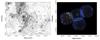 |
Fig. 1 Left: spatial distribution of X-ray sources detected by XMM-Newton (fields E, C, S and W; full lines) on the AV map (Cambrésy, priv. comm., 2000) with AV = 2.0 and 4.0 mag contours, compared with ROSAT fields from Gregorio-Hetem et al. (2009; dashed lines). Right: mosaic of images of XMM-Newton EPIC PN, MOS 1, and MOS 2 for the same CMa fields combined in three different energy bands. The red, green, and blue filters present the soft band (0.5–1.0 keV), medium band (1.0–2.0 keV), and hard band (2.0–7.3 keV), respectively. |
The method is now familiar. The X-rays come from high-mass stars owing to their strong wind shocks and also from the numerous young, low-mass stars (M⋆< 2 M⊙; T Tauri stars), owing to their magnetic activity and/or accretion, which may be present up to a relatively old age (~10 Myr, depending on their mass). Therefore, once they have lost their accretion disks (no IR excess, no Hα emission: ages ≥10 Myr), X-rays are the only way to identify the stars as being young. The ages are then derived using colour–magnitude diagrams and theoretical PMS evolutionary tracks.
The discovery of large samples of PMS stars has shown that many star-forming regions seem to have complex star formation histories, typically involving a sequence of individual episodes that created different subgroups or clusters. For an understanding of the star formation process, it is therefore of essential importance to look for young stars not only around the centre of a prominent cluster, but also to investigate its environment to detect and identify distinct stellar populations that often are found in separate clusters or groups of different ages.
One prominent example is the Scorpius-Centaurus OB association, where the individual subgroups are between ~5 Myr and ~15 Myr in age (Preibisch & Mamajek 2008). A similar situation, although with smaller age differences of just a few Myr, is seen in the subgroups of the Ori OB1 association (Bally 2008). The ~4 Myr stars of the Ori OB1c subgroup are seen in projection directly in front of the famous Orion nebula cluster and contaminate the cluster.
Another spectacular illustration of the diversity of young populations, not only in age, but also in space, is provided by the Chandra 22-field mosaic, ~1.4 sq. deg. survey of the Carina nebula (Townsley et al. 2011; Feigelson et al. 2011). In this nebula, the ~10 000 X-ray sources detected as young stars clearly belong to two distinct, equally numerous groups: a clustered population, with centrally concentrated distributions of stars (including cases of “clusters of clusters”), and a fairly homogeneous distributed fainter population. This is consistent with two main modes of star formation: localized cluster formation from dense molecular cores and more widely spread star formation from smaller condensations, for example “pillars” eroded by the hydrodynamical feedback from winds and/or supernova explosions from massive stars (M⋆> 8 M⊙), as in the Eagle nebula (Guarcello et al. 2010; Flagey et al. 2011). The various clusters and the distributed young stars in Carina nebula also show a large spread in ages (~1–10 Myr, depending on the location within the nebula).
Therefore, it is now clear, in particular from X-ray observations, that a large-scale picture of young clusters, and not only of a small area around their brightest members, is essential to reliably disentangle age and membership effects; in particular, the spatial mixing of stars that have different formation histories is essential, i.e. originating in distinct clusters or born via various feedback mechanisms at various epochs.
The above discussion raises crucial issues on star formation in clusters: what is the “real” membership of a cluster? And, which are the youngest and oldest member stars? The answer to the former is needed to build a reliable mass distribution and the latter to determine the global age distribution, and hence the duration of star formation in a given region.
These issues are not restricted to massive star-forming regions, but may apply to young clusters in general, hence fuel the ongoing debate on the duration of the star formation process (e.g. Palla 2011). Such a statement can be inferred for the CMa R1 star-forming region (d ~ 1 kpc) because it is a young complex that still has a lot of molecular material around and has star formation both finished and still ongoing, according to our previous results based on the wide field of ROSAT on the famous arc-shaped ionized nebula Sh2-296 (Gregorio-Hetem et al. 2009, hereafter Paper I). This nebula, of as yet unclear origin, comprises known young (~1–5 Myr) clusters, including around the famous binary (FU Ori-type + Herbig) star Z CMa. Figure 1 shows the two fields, covering more than ~2.7 deg2, where 98 X-ray sources were detected with ROSAT. A detection limit of FX = 5.0 × 10⁻¹⁵ erg s-1 cm-2 (log LX = 29.78) was achieved in Field 1 (exposure time of 20 ks), while observations in Field 2 were less sensitive because of a much shorter exposure (5 ks) (FX = 8.4 × 10⁻¹⁵ erg s-1 cm-2; log LX = 30).
Paper I reported the discovery of a previously unknown cluster of low-mass stars up to ~10 Myr in age called the “GU CMa cluster”, after the name of its brightest member. This cluster is located away from dense molecular material, indicating that star formation has now ceased in its vicinity. In contrast, the existence of several younger clusters on the other side of the CMa R1 molecular cloud, including around Z CMa, has been known for some time as a result of previous surveys at various wavelengths (see review by Gregorio-Hetem 2008). With respect to the molecular cloud, the GU CMa cluster therefore lies opposite to the Z CMa cluster, in a region devoid of molecular gas. The age gradient in each cluster and the similarity of the fraction of the intermediate-age populations (see Fig. 10 of Paper I) strongly suggests some degree of mixing between the two clusters. The young population in between Z CMa and GU CMa (the “inter-cluster” region) could be really mixed (i.e. coming from two distinct clusters, mixing at their edges) or perhaps could be indicative of the existence of an as yet unnoticed, distributed population on a large scale.
Results from Paper I motivated our group to propose new X-ray observations of CMa R1, which are more sensitive than those previously obtained with ROSAT in order to improve the identification of the entire young stellar population in this region. We have focussed on the “inter-cluster” region between the GU CMa and Z CMa subgroups (see XMM-Newton fields in Fig. 1) aiming to investigate if there is a mixing of their populations. Besides getting a more complete sample of the CMa R1 young stellar population we use the properties of X-ray and near-infrared emission of these sources to identify their nature and disentangle the scenario of star formation in this region.
The outline of the paper is as follows. In the next section, we describe the source detection and data reduction of the XMM-Newton observations, and the X-ray general properties are presented in Sect. 3. Section 4 is dedicated to the infrared analysis based on 2MASS and Wide-field Infrared Survey Explorer (WISE) data. A comparative analysis between X-rays and parameters derived from the infrared is performed in Sect. 5. Section 6 summarizes the results of this work. The general picture of star formation in CMa R1, extending the results from Paper I, is discussed in Sect. 7 and the main conclusions are presented in Sect. 8. Finally, Appendix A gives details about the analysis of the XMM-Newton data and Appendix B gives the complete catalogue of X-ray sources.
2. Observational data
For this work, four fields (each about 30 arcmin diameter with some overlap) were observed with the XMM-Newton satellite. These fields are located (Fig. 1) inside the arc-shaped ionized nebula, next to Z CMa – Field E (east); around GU CMa - Field W (west); and between both – Field C (centre) and Field S (south). The central coordinates from each field are given in Table 1. These observations were performed with the EPIC cameras (MOS1, MOS2, and PN) in full frame mode with a medium filter. The C, W, and S fields had an exposure time without background corrections of about 30 ks while field E had 40 ks.
These observations were analysed with the XMM-Newton Scientific Analysis System (SAS) version 11.0.0 software. The calibrated and concatenated events lists were obtained by epproc and empproc tasks applied to PN and MOS raw data, respectively. Fields E, W, and S were affected by high background activity, mainly in observations of the PN camera. In order to maximize the signal-to-noise ratio of weak sources, we created lists of clean events with the standard procedure for EPIC cameras that filters the background, removes flares, bad pixels, and bad events, and also reduces noise1. The good time intervals (GTI) of these observations are presented in Table 1.
Observing log for the XMM-Newton observations of CMa R1.
The source detection was performed in two steps: individually for each of the three EPIC cameras, and merging these cameras. In both cases, the detection was made in the three energy bands defined by Barrado et al. (2011): soft – SB2011 = 0.5–1.0 keV, medium – MB2011 = 1.0–2.0 keV, and hard – HB2011 = 2.0–7.3 keV. In order to distinguish young stars from field objects, different energy bands were tested and these were chosen because they are more efficient for the detection of (thermal) stellar sources. The images from the three cameras were created in each of these bands and also in the full energy range (0.5–7.3 keV). The right panel Fig. 1 shows a combined image obtained with EMOSAIC task, illustrating the three energy bands detections in PN+MOS images: SB2011 (red), MB2011 (green), and HB2011 (blue).
As a first step, the data from the three EPIC cameras were analysed separately via the SAS metatask EDETECT_CHAIN for source detection in each detector. This metatask creates exposure maps used to correct the images for the quantum efficiency, filter transmission, and mirror vignetting. It also provides detection maps that are used to perform sliding box detection with the locally estimated background. These sources are masked and background maps are created. Then, the metatask performs a second detection of sources using the background map and derives the parameters via a maximum likelihood method for each source. In order to explore softer energy bands, this procedure was also applied only to the PN data considering the energy bands suggested by Hasinger et al. (2001) as more efficient to detect (non-thermal) extragalactic sources; these bands are SH2001 = 0.2–0.5 keV, MH2001 = 0.5–2.0 keV, and HH2001 = 2.0–4.5 keV. However, the tests exploring these softer energy bands turned out to be less efficient for the detection of (thermal) stellar sources. For this reason we adopted 0.5 keV as lower limit.
As a second step, the images (corrected by exposure map) were divided by the effective area of the respective detector to take into account the differences in efficiency of the EPIC-PN and EPIC-MOS detectors. Then, with the EMOSAIC task, a combined image was created from these images for each energy band. Finally, the source detection was performed from combined image using the EMOSAICPROC metatask, which works similarly to the EDETECT_CHAIN taking into account the merged data from various observations and instruments, improving the source statistical significance and enabling detections of weak sources. However, this task only considers sources present in all combined instruments. A double check was applied in the individual images, searching for sources that were missed in the second step due to placement problems, such as falling outside of the field of view (FOV), inside a bad column, or near a gap of one or more of the instruments. In both cases the detection threshold was of maximum likelihood ML ≥ 15. Some sources were detected in two fields because fields E, W, and S are overlapping field C and, in these cases, we chose the sources with the highest signal-to-noise ratio.
The detection procedure has provided a catalogue containing 387 sources: 84 are in Field C, 187 in Field E, 79 in Field W, and 37 in Field S. Of these sources, 351 were detected using the merged images of all three cameras and 36 were detected by only one or two cameras. Table B.1 lists the X-ray detections and parameters for all sources in the four fields studied. These parameters are coordinates (J2000), maximum likelihood (ML) of source detection, count rate (CR) in the total energy band (0.5–7.3 keV), and hardness ratios HR1i = (Mi − Si)/(Mi + Si) and HR2i = (Hi − Mi)/(Hi + Mi). Here, Si, Mi, and Hi are the energy bands defined above, where the index i is related to the energy band ranges defined by B2011 and H2001.
Light curves and spectra were extracted only from EPIC-PN data with the standard SAS routines23. There are 47 sources in MOS 1/2 FOVs only, but none is bright enough for extraction of spectra and light curves. In both procedures the source and background regions were chosen by visual inspection, for each source. For the light curves we adopted the B2011 full energy range (0.5–7.3 keV) and time bins of 1000 s. The spectra were obtained in the full standard energy range (0.2–10 keV) suggested by SAS and were analysed using XSPEC version 12.7.1.
3. Results on X-ray properties
The X-ray data give us information related to the nature of the source, which is inferred from hardness ratios (HRs) diagrams, parameters derived from spectral analysis, and from the light curve. Appendix A gives more details on how these parameters were obtained from EPIC/PN data.
From HRs diagram analyses, based on B2011 and H2001 energy bands, we could classify 194 sources by comparing their X-ray emission with two model grids: thermal plasma, i.e. Astrophysical Plasma Emission Code (APEC; Smith et al. 2001) and a power-law (PWL)4 distribution, which are both multiplied by an absorption photoelectric model (PHABS)5. The sources that are compatible only with the APEC grid were classified as stellar objects, only 1/181 (0.5%) of these objects do not have IR counterpart. The sources compatible with a power law may have another origin as probably extragalactic or perhaps compact objects. There are 195 sources that we call “undefined”; 47 of these sources can be fitted by either the APEC or PWL model and 148 by neither model. According to the results from the infrared (2MASS + WISE) data analysis (see Sect. 5), we suggest that 84 sources remain as undefined objects: 23 probably are foreground stars and 17 have counterparts that are too faint (bad quality data), without confident classification. The other 44 undefined sources (11% of the XMM-Newton sample), which do not have 2MASS data, probably are background objects; this is in agreement with the expected 10% of contamination, at this level of sensitivity, mainly due to extragalactic sources (Getman et al. 2005a).
Source classification based on X-ray emission.
3.1. Light curves and spectra
Magnetically active stars, including T Tauri stars, typically show variable X-ray emission, for example, due to flare-like events varying from a few minutes (<30 min) to few hours (>8.5 h) and involving a large release of energy (1032 to 1035 erg/s, see Table A.1; Feigelson & Montmerle 1999; Favata & Micela 2003; Güdel 2004; Stelzer et al. 2007). In young stars, particularly T Tauri stars, the light curves of these events appear with different shapes (e.g. Favata et al. 2005; Wolk et al. 2005; Franciosini et al. 2007; Stelzer et al. 2007; López-Santiago et al. 2010).
Within our four ~30 ks exposures, 13 sources presented flare-like events, which we identified using the definition of a flare adopted from Franciosini et al. (2007) and Wolk et al. (2005), as described in Appendix A.2, which also presents all the light curves and flare parameters for these sources. The characteristics of flare-like events in this work are similar to T Tauri stars of the Taurus molecular cloud (e.g Stelzer et al. 2007), or young stellar objects (YSOs) from the η Chamaleontis cluster (López-Santiago et al. 2010). This similarity is shown in Fig. 2, which compares the energy and flare duration for our sample and these other regions.
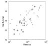 |
Fig. 2 Energy (Ef) and duration (Tf) of X-ray flares on CMa R1 sources (open circles) compared with those observed on members of Taurus molecular cloud (Stelzer et al. 2007), where classical and weak T Tauri are represented by filled circles and squares, respectively. Filled triangles show young stellar objects associated with the η Chamaleontis cluster (López-Santiago et al. 2010). |
In spite of the poor signal-to-noise ratio, we could perform the spectral fits of low resolution integrated spectrum for the whole exposure of some sources. The hydrogen column density, plasma temperature, and flux for non-flaring sources were obtained by fits of phabs × apec models for 21 sources, adopting metallicity Z = 0.2Z⊙, as appropriate for low-mass stars (see details in Appendix A.1). These spectra and parameters are presented in Appendix A.3. Their average hydrogen column density, NH = 1.8 ± 1.5 × 1021 cm-2, corresponds to an extinction AV = 0.9 ± 0.7 mag, by adopting NH/AV = 2.1 × 1021 cm2 (e.g. Vuong et al. 2003). This value is compatible with AV = 1.0 mag adopted in Paper I for CMa R1 and it is inside the range in which most of the sources are compatible with APEC model grids. The coronal temperatures, varying from 0.5 to 2.1 keV (6.7 < log T(K) < 7.4), are also compatible with those found in other star formation regions such as σ Orionis, η Chamaleontis (López-Santiago & Caballero 2008; López-Santiago et al. 2010), and the Pipe nebula (Forbrich et al. 2010). This means a low-extinction region, if compared with the minimum values for NH corresponding to AV = 0.4 for the foreground extinction in the direction of CMa R1, computed from the large-scale extinction models by Amôres & Lépine (2005), NH = 5.9 × 1021 cm-2 from LAB Map (Kalberla et al. 2005) and 6.9 × 1021 cm-2 from DL Map (Dickey & Lockman 1990).
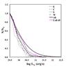 |
Fig. 3 Cumulative distribution of X-ray luminosities for sources in CMa R1 (black lines) and Collinder 69 (Barrado et al. 2011, magenta line). The thick grey line shows the log-normal distribution with μ = 29.3 and σ = 1 proposed by Feigelson et al. (2005). |
3.2. X-ray fluxes and luminosities
Based on the flux derived from the spectral fits of the brightest sources, we obtained the energy conversion factor (ECF) from the correlation between count rate and flux. The linear fits of these parameters gives a mean value of EFC = (1.60 ± 0.04) × 10-12 erg cm-2 cts-1 compatible with ECF = 1.56 × 10⁻¹² erg cm-2 cts-1 calculated by PIMMS6 for a 1-T thermal model adopting the mean values for plasma temperature and NH, derived from the EPIC/PN spectra (see Sect. 3.1).
The X-ray luminosities (LX) were derived from the fluxes for all the 340 sources detected by PN camera by adopting a distance of d = 1 kpc for CMa R1 (Shevchenko et al. 1999; Kaltcheva & Hilditch 2000; Paper I). Figure 3 shows the cumulative LX function (LXF) derived for each field. As further discussed (Sect.5), the presence of possible non-members contributes with low levels of X-ray emission that is not affecting the LXF. A thick line shows LXF for all sources, compared to the 5 Myr-old cluster Collinder 69 (Barrado et al. 2011) represented by the magenta line in Fig. 37. For both samples, whose data have similar sensitivity, the LXF cumulative distribution was derived taking into account detected sources with log LX(erg/s) > 29.5. As a guide, we add in Fig. 3 the log-normal distribution with μ = 29.3 and σ = 1, which is the “universal X-ray luminosity function” proposed by Feigelson et al. (2005). The differences on the distribution are found at the high luminosities end, mainly due to the low number of massive stars in our sample. This distribution is similar to the results for other low-mass clusters, such as Serpens and NGC 1333, for instance, discussed by Günther et al. (2012).
4. Analysis of infrared properties
The characterization of the X-ray sources needs to be complemented by observational data obtained in other wavelengths. For instance, Fernandes et al. (2015) performed a spectroscopic follow-up of optical counterparts for a partial sample of the XMM-Newton stellar sources associated with the Sh 2-296 nebula with the Gemini South telescope. Among 58 candidates, these authors found 41 confirmed T Tauri stars and 15 possible PMS stars (including intermediate-mass stars). Almost 50% of the young stars have less than 1 M⊙ and 35% have masses between 1–2 M⊙. While half of their sample is 1–2 Myr in age or less, only a small fraction (<10%) show evidence of IR excess indicating the presence of circumstellar disks. In comparison with other young star-forming regions (e.g. Haisch et al. 2001; Hernández et al. 2008; Fedele et al. 2010), this is a very low fraction of disk-bearing stars.
In order to expand the search for disk candidates among the X-ray sources associated with CMa R1, we analyse the near-infrared (NIR) counterparts of these sources using available data in the 2MASS and WISE (Wright et al. 2010) Catalogues. The method used to estimate the infrared properties is described in Sect. 4.1, in which we identify the NIR counterparts based on 2MASS data and use colour–colour and colour–magnitude diagrams to determine mass and age of the candidates. In the remainder of this section, we describe the IR classification (Sect. 4.2) determined with data from the AllWISE catalogue, the selection of a “best sample” by adopting mass and age criteria (Sect. 4.3), the analysis of mass function (Sect. 4.4), and age distribution (Sect. 4.5).
4.1. Near-infrared counterparts
We selected NIR counterparts by searching the 2MASS catalogue (Cutri et al. 2003) for candidates located less than 10′′ away from the nominal X-ray source positions. No counterpart was found for 45 sources. Candidates for which the distance seems to be incompatible with the cloud were disregarded. In the colour–magnitude diagram (see Fig. 4), these sources appear below the main sequence, indicating they probably are field stars.
The complete list of NIR counterpart candidates is given in Table B.2, but we consider as reliable only those with AAA flags in the 2MASS catalogue, i.e. magnitudes with high signal-noise ratio (S/N> 10), low errors (<0.1 mag), and above the completeness limit (J< 15.8, H< 15.1 and Ks< 14.7) ensuring good photometric quality (Lee et al. 2005). Table 3 gives the number of X-ray sources for each field and the corresponding number of their reliable NIR counterparts. Almost all are found less than 5′′ away from the centroid of the X-ray emission. This value has been used typically as a good estimate of the effective radius within ~90% confidence of the uncorrected positions (López-Santiago & Caballero 2008; Watson et al. 2003).
Number of sources with one (1) or more (2, 3) 2MASS counterparts.
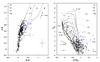 |
Fig. 4 Left: colour–colour diagram for all 340 2MASS counterparts of X-ray sources found in fields E, C, S, and W. Blue symbols represent disk-bearing (Class I and II) stars classified in Sect. 4.2. The ZAMS and locus of giant stars are indicated by thick lines, while the locus of T Tauri stars is represented by a thin line. Dotted and dashed lines show reddening vectors. Right: colour–magnitude diagram showing the isochrones 0.2, 1, 5, 10, 15, 20 Myr, and ZAMS (full lines), early main sequence (grey thick line) and evolutionary pre-MS tracks 0.1, 0.5, 1, 2, 3, 4, 5, 6, and 7 M⊙ (dashed line) from Siess et al. (2000). |
In total, we selected 340 reliable NIR counterparts to 290 X-ray sources, among which 46 have multiple counterpart candidates. Following Santos-Silva & Gregorio-Hetem (2012), we compare their positions in the colour–colour diagram (Fig. 4 left) with theoretical curves of the zero age main sequence (ZAMS) from Siess et al. (2000)8 and giants (Bessell & Brett 1988). Figure 4 (left) also includes an arrow that represents the reddening vector of AV = 2 mag (Rieke & Lebofsky 1985), the T Tauri stars locus (Meyer et al. 1997), and the regions defined by Jose et al. (2011) according to the NIR excess; stars with accretion disks are expected to be found in region “T” (Classical T Tauri stars: CTTS) and Class I protostars appear in region “P”. Field stars and diskless T Tauri stars (weak T Tauri stars; WTTS) that have little or no excess are mainly located in region “F”. Most of the counterparts are found in region F and/or near the ZAMS, indicating a low level of NIR excess for these sources.
Figure 4 (right) shows the colour–magnitude diagram (CMD) with reddening corrections made according to the extinction law from Cardelli et al. (1989) for AV = 0.9 mag, which is the mean value in the visual extinction map9 and corresponds to the average hydrogen column density (NH = 1.9 × 1021 cm-2), obtained from the X-ray spectrum fits (see Sects. 3.2 and A.3). The absolute magnitudes were estimated with the distance modulus mJ – MJ = 10 mag, according to the cloud distance adopted in Sect. 3.1 (d = 1 kpc).
The CMD shows theoretical isochrones for 0.2 to 20 Myr, ZAMS, and 0.1 to 7 M⊙ evolutionary tracks. We also included the early main sequence model that represents the last stage of evolution in the Siess et al. (2000) calculations (see Sect. 4.3). Mass and ages were estimated from comparison with the theoretical curves by interpolating the models, except for candidates appearing rightwards of the models in the CMD. According to the WISE data (analysed in Sect. 4.2), several of these candidates are Class I or Class II objects (see blue symbols in Fig. 4).
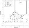 |
Fig. 5 WISE colours of counterparts of X-ray sources (dots) compared with the locus of Class I and Class II proposed by Koenig & Leisawitz (2014). Open symbols show objects classified according to their infrared excess, while crosses indicate known disk-bearing stars (Fernandes et al. 2015). |
4.2. Classification based on WISE data
Among our list of 340 NIR counterparts (Table 3), only 272 are also listed in the AllWISE data release (Cutri et al. 2013). However, we focussed the infrared classification on 157 objects with reliable WISE photometry, i.e. 115 sources with errors greater than 0.2 mag in Bands 1 (3.4 μm) and 2 (4.6 μm) and upper limits in Band 3 (12 μm) were not considered. In a first analysis, we looked for IR excess by combining the 2MASS and WISE data in the K-[4.6] versus H-K diagram.
The distribution of the 157 selected sources in this diagram revealed 34 objects with K-[4.6] > 0.7 mag, which is an indication of IR excess (Cusano et al. 2011; Fernandes et al. 2015) that could be due to the presence of a disk. This excess is in agreement with the colours of T Tauri and Herbig Ae/Be stars associated with Sh2-296 (Fernandes et al. 2015), which were included in this analysis (indicated by crosses in Fig. 5) as representative of known disk-bearing stars.
A more conclusive infrared classification was obtained with the criteria presented by Koenig & Leisawitz (2014) to classify YSOs based on WISE colours. Figure 5 shows the [3.4]–[4.6] versus [4.6]–[12] diagram and the Class I, II and III regions (dashed lines) defined according to the distribution of objects associated with the Taurus molecular cloud (Rebull et al. 2010). This analysis provided the separation of the 34 candidates, which show IR excess (K-[4.6] > 0.7 mag) in different types: 2 Class I, 19 Class II, and 13 Class II/ III. The other 123 NIR counterparts, which have good quality data but do not show IR excess, are considered Class III. Finally, the remaining 115 NIR counterparts with bad quality WISE data, to which we could not assign an infrared classification, are marked with “??” in the last column of Table B.2.
As we discuss further in Sect. 5.3, in spite of the youth of the sample associated with CMa R1, a low fraction (21/157 < 14%) of disk-bearing stars (Class I and Class II) is found, reinforcing the previous partial results of Fernandes et al. (2015).
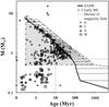 |
Fig. 6 “Best sample” of X-ray sources based on estimates of masses and ages for 340 2MASS counterparts (see Table B.2). This sample, which takes into account the incompleteness of our sample below ~0.5 M⊙, are present in the grey area. The empty area between dotted lines corresponding to the mass range 0.5–0.7 M⊙ and age >10 Myr is interpreted as the decline of magnetic activity of low-mass young stars with age (see Sect. 7.2). |
4.3. Defining a “best sample” of XMM-Newton sources
As a consequence of the dependence of X-ray luminosity on stellar mass, the selection of our sample naturally imposes a mass detection threshold. More precisely, owing to our XMM-Newton detection limit (see below, Sect. 5.2) and in comparison with other X-ray observations of star-forming regions, our list of X-ray sources is incomplete for low-mass stars. In order to statistically improve the analysis of the 2MASS data, we adopted conservative criteria searching for NIR sources, which restrict the counterparts selection to the reliable candidates where the source sample is complete, i.e. our so-called “best sample”.
The selection criteria are based on Fig. 6, which compares masses and ages of our candidates with theoretical values interpolated from the ZAMS and early main sequence evolutionary tracks from Siess et al. (2000). According to these authors, this last track is more representative of stars with mass >1.2 M⊙ having reached equilibrium after the CNO cycle. This is the last stage of evolution in the Siess calculations, occurring after the ZAMS, and corresponds to the end of deuterium burning, when the nuclear energy production switches to hydrogen burning and starts to provide all the stellar luminosity. Considering that our sample is complete only in the ranges of 0.5 < mass (M⊙) < 9 and 0.3 < age (Myr) < ZAMS, when taking into account the XMM-Newton detection limit for CMa R1 (see Sect. 5.1 and Fig. 10), our final “best sample” is highlighted by the hatched region in Fig. 6. By adopting this criterion, the NIR analysis is restricted to 225 counterparts (comprising multiples): 122 of these counterparts belong to field E, 37 to field C, 23 to field S, and 43 to field W.
It is important to stress that the other sources (appearing outside the hatched region of Fig. 6) remain as possible counterparts of the X-ray sources. These sources were removed from the present analysis only to obtain more conclusive results based on a limited, but complete sample (in a given range of mass and age), rather than on a larger, but incomplete, sample, as explained above.
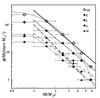 |
Fig. 7 Observed mass distribution indicated by various symbols with error bars. The lines represent the power-law fitting of mass function φ(M) for M> 1M⊙ of individual XMM-Newton fields E (dashed), C (dot dashed), S (long dashed), and W (dotted), and considering the entire “best sample” (black). The grey line shows the theoretical log-normal curve proposed by Chabrier (2005) with μ = 0.3 and σ = 0.6. |
4.4. Mass function
Considering the four XMM-Newton fields together, we find that over 75% of stars have masses 0.5 <M(M⊙) < 2, together with a few massive stars. In order to examine differences and similarities in the mass distribution of each field we calculate their cumulative mass function, which we write in the form φ(M) ∝ M− (1 + χ). According to Krumholz (2014), for young stellar clusters the mass function is essentially identical to the initial mass function (IMF), so we can directly compare our mass functions with theoretical models of IMF, such as Salpeter (1955), Kroupa (2001), and Chabrier (2005). According to these authors, the IMF for stars with masses larger than 1 M⊙ can be represented by a power-law function with a slope χ ~ 1.35, while for low-mass stars Kroupa (2001) suggests broken power-law functions with χ = 1.3 (0.5–1 M⊙) and χ = 0.3 (0.08–0.5 M⊙). Chabrier (2005) suggests a log-normal distribution with peak at ~0.2–0.3 M⊙ and a dispersion of ~0.5–0.6 M⊙. A good discussion about the differences among these models is presented by Bastian & Meyer (2010).
Figure 7 shows the observed φ(M) and slopes obtained for each XMM-Newton field. Aiming to compare our results with the theoretical power-law function (valid for M> 1M⊙), the fit to the slope of φ(M) does not include stars with 0.5 <M(M⊙) < 1. The mean value of χ = 1.27 ± 0.09 obtained for the entire sample is consistent with the Salpeter IMF and agrees with the models of Kroupa (2001) and Chabrier (2005), although it differs somewhat from the values estimated for each field; i.e. 1.21 ± 0.11 (Field E), 0.97 ± 0.14 (Field C), 1.08 ± 0.09 (Field S), and 1.73 ± 0.14 (Field W). Since our “best sample” is complete for M> 0.5 M⊙, the turnover below 1 M⊙ is real and consistent with the log-normal distribution proposed by Chabrier (2005) as shown in Fig. 7. In this case, the theoretical curve, a log-normal function with μ = 0.3 and σ = 0.6, is compared with the distribution of all sources of the “best sample”.
Altogether, except for Field W, which has a definitely steeper slope, all fields have mass function slopes comparable to those of other young stellar clusters studied by Santos-Silva & Gregorio-Hetem (2012); for instance, Collinder 205, Lyngå 14, NGC 2362, NGC 2367, NGC 2645, NGC 3572, NGC 3590, NGC 6178, Stock 13, and Stock 16.
4.5. Age distribution
The histograms in Fig. 8 show, for each field, the distribution of objects in three age ranges. The main differences are in Fields E and C where about 50% of the sources have ages between 0.3 and 5 Myr, while in Fields S and W more than 55% of the objects are between 10 Myr in age and ZAMS. Even considering the 43 NIR counterparts that were discarded for lack of age information (see Sect. 4.1), the distribution follows the same trend, since their NIR-excess suggests they probably are < 0.3 Myr. In this case, the fraction of sources with ages <5 Myr in Fields E and C would be more than 60%, not affecting the distribution of Fields S and W.
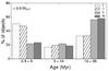 |
Fig. 8 Comparison of age distributions for each field considering three ranges of age. |
Although we discuss each field separately, it is important to keep in mind that this division is purely observational because it is based on the selection of the XMM-Newton pointing directions. However, they do reflect, to some extent, different stellar populations, since the fields were selected on the basis of our previous ROSAT observations ( Paper I). So the large differences apparent in the histogram of Fig. 8 are statistically significant and indicative of real differences in the stellar populations within the CMa R1 region. In particular, these results fully confirm and extend the age distribution obtained in Paper I, in which, in particular, the group next to CMa GU (age >10 Myr) appears significantly more evolved than the group near Z CMa (age <5 Myr) with a mixture of ages in between.
5. Comparison of X-ray and NIR properties
As described in the previous sections, X-ray and NIR data have revealed that most (79%) of the XMM-Newton sources are probable members of CMa R1. The combination of the results from both analyses can confirm their young nature. On the other hand, 21% of the XMM-Newton sample are probably field objects. Among these, 6% (23/387) have infrared counterparts that probably are foreground stars and 4% (17/387) have counterparts that are too faint (bad quality data) without reliable classification. The other 11% of undefined sources (44/387) do not have 2MASS data because they are classified as possible background objects. We have seen that the XMM-Newton error boxes may include multiple NIR counterparts, so we restrict the comparative analysis described in this section to the 158 X-ray sources of our “best sample” that are associated with a single NIR counterpart.
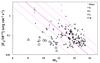 |
Fig. 9 X-ray fluxes (FX) vs. magnitude in 2MASS J band (mJ). The solid line presents the relationship log (FX) = − 9.8( ± 0.4) − 0,33mJ similar to that obtained using ROSAT data in Paper I. The large symbols represent Herbig Ae/Be stars (M> 2M⊙). Dotted and dashed lines show 1σ and 2σ offset, respectively. |
5.1. X-ray flux versus J-band magnitudes
Based on ROSAT sources detected in CMaR1, in Paper I a correlation between X-ray luminosities and absolute magnitude in J band (=1.24 μm) was presented: log LX = 31( ± 0.4) − 0.33 MJ, which is similar to the results for T Tauri stars associated with nearby clouds such as Chamaeleon (Feigelson et al. 1993) and ρ Ophiuchi (Casanova et al. 1995). Compact stars and extragalactic objects are expected to appear above this correlation, since their X-ray emission is comparatively much more intense relative to their NIR luminosity. Herbig Ae/Be stars, which have lower levels of X-ray flux, when compared to their NIR emission, show the opposite, appearing below the T Tauri correlation, in spite of the age similarities for these two types of PMS stars.
Considering that 1 keV (the typical energy peak of our sources) and the J band coincidently have almost exactly the same extinction cross-section (Ryter 1996), we opted for a direct comparison between X-ray flux and apparent J magnitude, avoiding inaccuracies due to errors on the extinction estimation that affects luminosity and absolute magnitude estimation.
In this case, the correlation given in Paper I can be expressed by log FX = − 9.8( ± 0.4) − 0.33 mJ, where FX is given in erg s-1 cm-2. A comparison of our sample with this correlation is presented in Fig. 9, where the sources showing flares are highlighted. The error bars shown in the top left of Fig. 9 correspond to less than 30% of the flux and 0.1 in magnitude, which are representative of our “best sample”.
Most sources of our sample roughly follow the empirical correlation within 2σ deviation. Only seven sources have a larger deviation, but they are not real outliers. Three of these sources are associated with flare events, which is not unexpected since flares release a large amount of energy, resulting in a higher X-ray flux than that emitted by the source in quiescence, but are too hot to affect the NIR emission. The other four objects (three in Field E and one in S) found above the correlation may be unresolved multiple systems with faint companions. In fact, one of these objects has been identified by Fernandes et al. (2015) as a binary system, in which both companions were classified as WTTS. The fainter star in the binary was not included in our sample of NIR counterparts owing to the low quality of NIR data. Based on the number of X-ray sources with two or more NIR counterpart candidates, we estimate less than 8% (17/206) of possible (not confirmed) binaries in our “best sample”.
On the other hand, 13 sources lie below a 2σ deviation from the correlation because they have low FX but high values of mJ. Large symbols are used to represent these sources, which more likely coincide with the expected region for Herbig Ae/Be stars in Fig. 9. This hypothesis is reinforced by the high mass of these objects, which varies from 2.1 to 6.2 M⊙.
We conclude that, based on the correlation for T Tauri stars shown in Fig. 9, all the sources in this sample can convincingly be considered as YSOs.
5.2. Masses and X-ray luminosities
The distribution of LX as a function of mass was compared to that of other young clusters and star-forming regions such as the Orion nebula cluster (ONC; Preibisch et al. 2005), the Taurus molecular clouds (TMC; Güdel et al. 2007) and Collinder 69 (Barrado et al. 2011). A summary of lower limits of X-ray luminosities and fluxes, as well as target distances and exposure times of the X-ray observations used in this comparison are presented in Table 4.
Limits in X-ray observations.
The ONC and TMC are closer than CMa R1 and some of their X-ray observations were performed with longer exposure times. Therefore the capability to detect fainter sources results in a more complete sampling of the lower mass end of their population (see Table 4). For comparison, the detection limit of our sample is illustrated in Fig. 10.
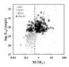 |
Fig. 10 X-ray luminosity vs. stellar mass for the sources in CMa R1 (black triangles) compared with T Tauri stars in other star-forming regions: Orion nebula cluster (ONC), Taurus molecular cloud (TMC), and Collinder 69 (Coll69). The dashed line indicates the limit of mass adopted to define our “best sample”. The gap at 0.4–0.5 M⊙ is not real, but due to difficulties in interpolating models on this mass range. |
The minimum flux detected in the other regions is 10 to 100 times lower than that of CMa R1, clearly suggesting the absence of faint X-ray emitters among our sample, which implies that a considerable number of low-mass stars (<0.5 M⊙) are below our detection limit, especially if we compare the masses and luminosities of sources in our sample with TMC objects.
The differences and similarities of the LXF derived in Sect. 3.2 for each field compared to the Collinder 69 cluster considering the same mass range (see Fig. 3). The LXF for all the CMa R1 sources has slightly lower X-ray levels than Collinder 69, which has most of the members with 5 Myr and masses <2 M⊙. In this case, the differences in X-ray properties depend not only on the larger range of ages of our sample, but also on the masses. As indicated in Fig. 9, intermediate-mass young stars tend to have lower X-ray emission when compared with the FX versus mJ correlation found for low-mass stars. This can also be seen by the relatively higher proportion of sources found in Field C (~19%), appearing below the 1σ correlation in Fig. 9, when compared to Field E fraction of sources (<6%), which also reflects to the fainter LXF presented by field C. Since the fraction of young stars (<5 Myr) is similar for both fields, it is not an age effect but differences in mass distribution. As shown in Fig. 7, there is a lack of stars more massive than 4 M⊙ in field C, giving a less steep slope if compared with the mass distribution in Field E.
5.3. Comparison with dust and dense gas distributions
As discussed in Sect. 4 there is a low fraction of stars with IR excess, which are those appearing to the right of the vector indicated by the dotted line in the 2MASS colour–colour diagram (see Fig. 4). When considering the whole sample of 2MASS counterparts only 8.5% (29/340) have a K-band excess. The analysis based on WISE data shows 22% (34/157) of the sample with K-[4.6] > 0.7 mag that we considered disk-bearing candidates, however, only two of these candidates were confirmed as Class I objects and 19 are Class II. This small number of Class I protostars and Class II T Tauri stars candidates in the XMM-Newton fields is also confirmed by a census of YSOs covering the whole CMa OB1 star-forming region (10° × 10°) performed by Fischer et al. (2016). These authors follow a slightly modified version of the criteria suggested by Koenig & Leisawitz (2014). Nevertheless, they use WISE colours similar to those adopted by us (Sect. 4.2); in the list of Fischer et al. (2016) a smaller number of disk-bearing stars, 1 Class I, and 11 Class II, are found to coincide with the X-ray sources. Their census is not complete for the XMM-Newton surveyed area, probably due to their more restrictive criteria in excluding WISE sources that show any contamination flag.
The spatial distribution of the NIR counterparts is analysed in Fig. 11 to look for evidence of clustering. In spite of the fact that the fields observed with XMM-Newton were not meant to correspond exactly to physically separated clusters or stellar groups, their location turns out to reflect fairly accurately the spatial distribution of the sources as a function of position (in projection). Roughly, Field E contains sources located on the inner side of the cloud, Fields C and S contain sources distributed along the border of the visible nebula, while most of the Field W sources are outside the molecular cloud.
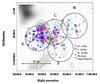 |
Fig. 11 Spatial distribution of NIR counterpart of X-ray sources as a function of age. This is compared to a 13CO map10 shown by the grey image superimposed on AV> 2 and 4 mag contours (the same as Fig. 1). The diamonds, squares, and circles represent objects with less than 5 Myr, between 5 and 10 Myr, and more than 10 Myr, respectively. The counterparts found outside of Siess et al. (2000) PMS isochrones are represented by crosses and disk-bearing candidates (see Sect. 4.1) are shown by blue ellipses. Black circles delimit the fields E, C, S, and W. |
The position of the sources in Fig. 11 is also compared to the cloud gas distribution, revealed by 13CO map10, where dense areas coincide with the dust distribution, (as seen in Fig. 1) indicated by the AV map9. Field W is dominated by older objects (>10 Myr; circles), without preferential distribution. On the other hand, Fields E and C show a mixing of all age ranges and objects without well-defined age (represented by crosses). In Field C, most of the younger objects (<5 Myr) are within the area with the highest concentration of CO, while in field S younger objects are on the edge or outside the CO contours. In both cases we can see a segregation of ages, in which most of the older sources are found on the right side towards GU CMa, and younger sources are found on the left side, near the edge of the nebula. However, young objects are also found in the empty area around GU CMa, while older objects are also found in the dense area around Z CMa, pointing to an apparent paradox in the history of star formation in the CMa R1 region.
About 70% of NIR counterparts with K-band excess and all disk-bearing candidates found in Fischer et al. (2016) are distributed in regions with high 13CO flux (>20 Jy), which is also the location of dust concentration responsible for the extinction. Since a uniform value AV = 0.9 mag has been adopted in the present work, it is possible that the reddening correction was too small for these sources. Several of these sources are located in the area of the BRC 27 and VDB RN92 clusters that have AV = 6.5 and 4.4 mag, respectively (Soares & Bica 2002, 2003). A more detailed estimate of individual values of AV could help us better determine the ages and masses for such embedded objects and probably increase the sample of bona fide CMa R1 members. We defer such a study to a future paper.
6. Summary of the results
Our observations performed with XMM-Newton resulted in a sample of 387 X-ray sources (187, 84, 37, and 79 in Fields E, C, S, and W, respectively), 340 of which have one or more NIR (2MASS) counterparts.
In order to characterize the CMa R1 members, we made complementary use of the X-ray and NIR data. We compared the X-ray hardness ratios to a model grid for a hot thermal plasma and for power-law spectra that we simulated with XSPEC and we compared the NIR photometry to the isochrones from PMS evolutionary models.
Based on results from the X-ray analysis, summarized in Table 2, the sources were separated according their HRs: 47% are well reproduced by a thermal plasma (APEC model), as expected for stars, and 3% probably are extragalactic sources (power-law model). The other half of the sample could not be identified in one of these categories because 12% are reproduced by both models and 38% are outside the grids. As described below, the numbers of probable members or field objects were refined in agreement with the analysis of NIR counterparts. Moreover we could obtain more X-ray properties of several sources through their light curves and spectra. About 13 sources show flare-like events and the 21 brightest sources had their plasma parameters determined by fits of the low resolution EPIC/PN spectrum with an APEC model. The results from the spectra of these bright sources were used to determine the energy factor conversion and consequently the X-ray luminosities.
Among the NIR counterparts, 225 were selected to define our so-called “best sample”. The fits of the mass distribution φ(M), assumed to be a power law of the form φ(M) ∝ M− (1 + χ), give a slope χ ~ 1.3 ± 0.1 for stars more massive than 1 M⊙, which is consistent with the Salpeter IMF and in agreement with theoretical and observational results from the literature. Almost no difference is found among the observed fields when comparing their individual mass function, except of Field W, which has a lower fraction of stars more massive than 4 M⊙ with respect to its fraction of low-mass stars, increasing its slope. Most of the younger sources (<5 Myr) are present in Fields E and C, while about 60% of older sources (>10 Myr) are in Fields W and S. All the fields have almost the same proportion (~20%) of objects with intermediated ages (5–10 Myr).
The comparison with the X-ray flux and J magnitude correlation found for T Tauri stars or Herbig Ae/Be stars was restricted to the 158 sources of our “best sample” having a single NIR counterpart. Most of these sources follow the FX versus mJ correlation, except for 13 found below this correlation, which are probably Herbig Ae/Be stars as confirmed by their mass 2 < M(M⊙) < 8. For 7 sources that are above this correlation, three are in a flaring state and four have anomalous light curves, meaning that two or more peaks of X-ray flux, followed by a decline, were detected when compared to the quiescent state.
Compared with other young stellar clusters, our sample shows a typical distribution of X-ray luminosities as a function of mass. However, the sample is incomplete for low-mass stars, mainly those that are faint X-ray emitters. Our survey was only able to detect objects with log(LX [erg/s]) > 29.5, which results in an apparent deficiency of young stars with masses <0.5 M⊙. Another possible cause for incompleteness is related to the fact that about 10% of the X-ray sources may be low-mass stars affected by high levels of visual extinction. Most of these stars are located in the direction of dense regions of the 13CO map10, which prevented estimates of mass and age in this case.
By combining the two methods, X-rays and NIR, we propose a classification of the XMM-Newton sources into three groups: (i) CMa R1 members, which are very likely associated with the region because they have X-ray HRs compatible with a thermal plasma model and belong to our “best sample” of NIR counterparts; (ii) possible CMa R1 members, which were considered young according to only one of the methods; and (iii) undefined sources, whose origin we could not determine by any of the methods or sources rejected by at least one method. The number of classified sources in each group is shown in Table 5. Among the undefined sources there are 44 (11% of the total XMM-Newton sample) that we estimate to be extragalactic (background) because of the lack of NIR counterpart, 23 (6%) objects with NIR colours of field stars (foreground), and 17 (4%) with counterparts that have bad quality 2MASS data, giving them an inconclusive classification.
The optical spectroscopy performed with Gemini South by Fernandes et al. (2015) covered 40 of our sources in Field E. Among the CMa R1 members (M) and possible members (P) classified by us, 22 and 18, respectively, were confirmed as PMS objects. Moreover, all Class I, II, and III objects, based on WISE data, are also found among M and P sources of Table 5.
This agreement also proves the efficiency of the methods adopted in this work to identify the members of CMa R1.
Number of CMa R1 candidate members.
7. Discussion
In order to obtain a comparative and wider view of the young stellar population in CMa R1, we include in the present discussion some additional objects selected from Paper I on the basis of their ROSAT observations.
Number of X-ray sources as a function of age and mass ranges and their spatial distribution.
A simple comparison of the spatial density of detected sources in both surveys gives an immediate appreciation of how much the sensitivity improved with the present XMM-Newton observations (yielding ~550 sources deg-2) over the previous ROSAT results (~36 sources deg-2). However, the ROSAT sources were detected in a larger FOV (~2.7 deg2) while the total area covered by XMM-Newton for the present work is five times smaller (~0.7 deg2).
An overview of the spatial distribution of the total number of 250 young stars selected as our enlarged “best sample” (225 XMM-Newton + 25 ROSAT) indicates that 171 (68%) are seen close to Z CMa, superimposed on the east side the of AV> 2 mag contour shown in Fig. 12, while 79 are found on the west side of AV contour, around GU CMa, in areas devoid of molecular gas (AV ~ 0.5 mag). In the next sections, the location of the sources is discussed relative to their ages and masses as obtained in Sect. 4.1 for our sample and in Paper I for ROSAT sources, and to the distribution of dense gas over a wider area than that covered by XMM-Newton alone.
7.1. Spatial distribution versus stellar ages
With the purpose of investigating the spatial distribution of our sample of young stars relative to their age, Table 6 gives the number of XMM-Newton sources supplemented by ROSAT sources, separated in three age ranges; these are the same sources as found in Fig 8; i.e. 0.3–5 Myr, younger stars; 5–10 Myr , intermediate-age stars, and 10–55 Myr, older stars. Based on these definitions, the fraction of ~40% of the younger stars observed by XMM-Newton, which is similar to that of the older stars, is thus in agreement with Paper I (their Fig. 10, top left panel) based on ROSAT observations of a much smaller source sample, which gives 45% and 35%, respectively, in spite of the differences in sensitivity and FOV. This means that this age distribution is very robust and gives a good characterization of the X-ray detected young stars as a whole, over a large area.
The spatial distribution of objects was also examined relative to their position with respect to the gas based on the comparison with the density contours of the CO map shown in Fig. 12. The last two columns of Table 6 give the number of objects seen in front of dense parts of the cloud (“east” side, around Z CMa) or of regions devoid of gas (“west” side, around GU CMa).
This study yields what seem to be paradoxical results. On the one hand, we can clearly see an expected correlation between the ages of stars and their relation with star formation sites: the youngest stars are spatially correlated with dense gaseous regions of the cloud, as it is observed in, for example ONC and OMC2/3 regions (Megeath et al. 2012; Gutermuth et al. 2011), while older stars are spread where the gas is absent. On the other hand, we also find young stars in the empty regions (30%) and older stars in the dense regions (34%), while intermediate-age stars (19%) are found everywhere. To help understand this paradox, we now turn to the distribution of stellar masses.
7.2. Spatial distribution versus stellar masses
As in the previous Section, we separate the sources in three ranges of mass as shown in panels d, e, and f of Fig. 12. The number of objects in each range is given in Table 7. When comparing the overall mass distribution of XMM-Newton sources with that obtained from ROSAT ( Paper I), we find comparable fractions of stars in the ranges 1–2 M⊙ and >2 M⊙ in ~55% and ~30% of the ROSAT sources, respectively (see Paper I, Fig. 10, top right panel). As expected because of their different sensitivities, the main difference is found for low-mass stars (0.5 to 1 M⊙), for which the fraction in the ROSAT list is three times lower (15%) than in the present work (41%).
The spatial distribution of the stars found on both sides of the cloud (see the last two columns of Table 6) shows a trend (34/53) for the higher stellar masses to be more concentrated in the dense, east side in the vicinity of Z CMa. More precisely, Fig. 12d shows the stellar mass interval 2–9 M⊙ broken down in three mass ranges, i.e. 2–3 M⊙, 3–5 M⊙, and 5–9 M⊙ for XMM-Newton sources. For all these ranges, the XMM-Newton field E, overlapping Z CMa, is more populated than the other fields. On the other hand, the ROSAT data, for which the masses cannot be determined as accurately as from XMM-Newton data, show that high-mass stars (2–9 M⊙), which normally are closer to dense matter since they are younger, do exist also far from the main cloud. Intermediate-mass stars (Fig. 12e: 1–2 M⊙) are more evenly distributed on both sides of the cloud and are very numerous also in the empty regions of ROSAT field, far from the cloud. In contrast, Fig. 12f shows a decline of low-mass stars towards the empty, west side of the cloud as detected by XMM-Newton, and no low-mass stars in the ROSAT field further out.
This strong effect cannot be entirely due to the comparatively low sensitivity of the ROSAT observations. It is true that, as mentioned in Table 4, the ROSAT observations in this area are 0.3 dex less sensitive than the east field XMM-Newton observation (a factor of 2 in luminosity), and therefore the ROSAT census of low-mass stars (M⋆< 1M⊙) cannot be complete. Nevertheless, as shown by Table 6, where we indicated the sources detected both by ROSAT and XMM-Newton, we see that in total 15 low-mass stars have been successfully detected by ROSAT, but only 4 (~25%) were detected in the area defined by the XMM-Newton Field W, and none were detected beyond this area. Since we see in all the other panels of Fig. 12 that there are many ROSAT detections outside of the XMM-Newton fields, this effect must be real.
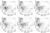 |
Fig. 12 Spatial distribution of NIR counterparts compared with the visual extinction map9. The lowest contours indicate a separation of dense regions (AV> 2). The diamonds and crosses represent XMM-Newton and ROSAT sources, respectively. Top panels a–c show objects with less than 5 Myr, 5 to 10 Myr, and more than 10 Myr, respectively. Bottom panels d–f are objects with masses larger than 2 M⊙, 1 to 2 M⊙ and between 0.5 to 1 M⊙, in this panel are highlighted XMM-Newton objects with masses between 2 and 3 M⊙ (diamonds), 3 and 5 M⊙ (X), and more than 5 M⊙ (full diamonds). Black full lines delimit the fields E, C, S, and W and the ROSAT field is indicated by a dashed line. |
To look in greater detail at this apparently different behaviour in our X-ray detection of low-mass stars compared to higher mass stars, we created a set of three figures (Figs. 13a–c), corresponding to the same late age range as Fig. 12c (10–55 Myr), but broken down in three low-mass ranges (0.5–1 M⊙, 0.5–0.8 M⊙, and 0.5–0.7 M⊙, respectively). We also include, for each panel, the ROSAT detections, even if they correspond to XMM-Newton detections as well. First, we see a very clear trend for the number of sources to diminish towards lower masses. There are only two XMM-Newton detections left and no ROSAT detection below 0.7 M⊙, compared with 39 XMM-Newton and 4 ROSAT detections below 1 M⊙. Second, even though we know the ROSAT sample is incomplete below 1 M⊙, we still have 3 ROSAT detections (and 14 XMM-Newton) between 0.5 and 0.8 M⊙. However, irrespective of the (low-mass) range, there is no detection in the ROSAT field outside of the XMM-Newton fields. Third, this effect corresponds to the empty area visible in the mass-age scatter plot for our “best sample” of XMM-Newton sources (Fig. 6), for M⋆< 0.7M⊙ and age > 10 Myr. Such an effect is not expected in the ROSAT data because of its incompleteness in this mass range.
In fact, there is a physical reason for this behaviour of low-mass stars. The study by Preibisch & Feigelson (2005) on the evolution of X-ray emission in young stars spanning the 1–10 Myr age range, which covers very young clusters in Orion (COUP; Getman et al. 2005b), NGC 2264 and Chamaeleon and is supplemented by older, open clusters (Pleiades, Hyades) extending the ages to 650 Myr, has shown two regimes. During the PMS phase (up to ~10 Myr), the X-ray luminosity is roughly constant for all masses, which corresponds to the “saturated phase” in which the young stars are fully convective. Then a radiative core develops and beyond 10 Myr the X-ray luminosity decreases abruptly (see their Fig. 4) in relation with the stellar spin-down (link with the magnetic field generation by the αΩ dynamo; see also Vidotto et al. 2014). Preibisch & Feigelson (2005) show that, for masses M⋆ = 0.5–0.9 M⊙, the median X-ray luminosity ⟨ LX ⟩ (in erg s-1) declines from ⟨ log LX ⟩ ~ 30 between 1 and ~10 Myr (ONC, NGC 2264, and Chamaeleon), down to ⟨ log LX ⟩ ~ 29 at ~100 Myr (Pleiades and Hyades). The slope of the decline is steeper for higher masses11. So in our case, given the sensitivity of our X-ray observations (log LX ~ 29.3–29.5 for XMM; see Table 4), we interpret the empty area of Fig. 6 as evidence for this decline in magnetic activity at >10 Myr for M⋆< 0.7M⊙.
Consequently, the west side of the cloud very likely contains low-mass stars, but these were formed over 10 Myr ago in an earlier episode of star formation and are now too faint to be visible in our observations. In fact, several objects detected by WISE appear in this side of the cloud, without IR excess, hence these objects may be Class III or field stars.
More precisely, since the WISE detections imply the existence of faint, evolved circumstellar disks (debris and/or planet-forming), the corresponding stars are classified Class II/III, and it is worth considering whether their presence affects their detectability in X-rays (i.e. their magnetic activity), in addition to, or instead of, the change in internal structure at ages ~10 Myr. First, with reference to Fig. 13a (M⋆ = 0.5–1.0 M⊙), we find 14 XMM sources to the west of the cloud complex (AV< 2), 3 are <10 Myr in age, and 11 are >10 Myr in age. However, of these only 5 have a WISE classification: below 10 Myr, 2 sources are Class III (no disk), above 10 Myr 1 is Class II/III, and 2 are Class III. Within this small sample, the difference is not significant. To increase the statistics, we can enlarge the sample in mass. For the range M⋆ = 0.5 − 2.0 M⊙, we find 19 sources with a WISE classification; i.e. 1 Class II/III versus 7 Class III for ages <10 Myr, and 1 Class II/III versus 10 Class III for ages >10 Myr, respectively, so the difference in diskless stars (7 versus 10) is again not significant. In other words, the decline in magnetic activity after ~10 Myr equally affects the X-ray detectability of low-mass stars, whether or not they are surrounded by (evolved) disks.
8. Conclusions
We focus our main conclusions on two issues: first, a major observational contribution, which has increased the known census of the stellar population associated with CMa R1 by a factor 15, and second, the implication of these results to unveil its complex star formation history. By discussing the interplay between star formation and molecular clouds that probably dictated the scenario of this history, we aim to shed some light on the role of stellar feedback on molecular clouds, which is an open issue on the general context of star formation in the Galaxy.
In a study on the reliability of age measurements for YSOs, Preibisch (2012) points out the debate in the literature concerning the timescale of star formation. Some authors argue that star formation should be a “fast”, dynamic process (e.g. Hartmann et al. 2001; Elmegreen 2007; Dib et al. 2010), while an opposite view of a “slow” quasi-static equilibrium process has also been discussed (e.g. Palla & Stahler 2000; Tan et al. 2006; Huff & Stahler 2007; Palla 2011). Testing these theories depends on the estimate of star-forming duration and a good determination of the age spread of the YSO population.
The presence of a relatively old population in the whole area (i.e. both the dense gaseous and empty sides of the cloud)
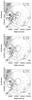 |
Fig. 13 Same as Fig. 12c (spatial distribution in the age range 10–55 Myr), but for low-mass stars only. In the three panels (a–c), the stellar masses are broken down in three mass ranges (0.5–1 M⊙, 0.5–0.8 M⊙, 0.5–0.7 M⊙, respectively), black diamonds represents XMM-Newton sources, and crosses indicate ROSAT sources. As discussed in the text (Sect. 7.2) and as is visible in Fig. 6, the nearly complete absence of stars with M <0.7 M⊙ is due to the decline of their magnetic activity after ~10 Myr. |
suggests that stars were slowly formed in a first episode throughout the region >10 Myr ago. As argued above, the older low-mass stars are not seen in the west side because their X-ray emission has fallen below our detection limit. Massive stars (M⋆< 9 M⊙) are however present in this area, but are younger than 10 Myr and are absent at older ages. Since these stars have a lifetime ~40 Myr, more massive stars, i.e. M⋆> 10 M⊙, have a lifetime <40–10 = 30 Myr, consistent with the current IMF (Fig. 7); these massive stars may have existed then exploded, dispersing the molecular clouds and possibly preventing the formation of new stars. Of course, after such a long time (30 Myr ago), one can hardly expect to see any trace of the explosion(s), precisely because the masses and spatial distribution of the molecular clouds must have been very different from what they are now.
We avoid being affected by these difficulties in the age determinations by being able to break down the ages into less precise, but broader ranges. Indeed, we found a true bimodal distribution of ages with two clearly distinct groups: one is younger (<5 Myr) and the other is older (>10 Myr) with less than 20% of the objects in the intermediate age range (5–10 Myr). Therefore, our results show that at least two star formation episodes took place in the same region, separated by at least ~5 Myr.
The older low-mass stars, as well as their putative associated high-mass O stars, are however not seen in the west side: the former because their X-ray emission has fallen below our detection limit and the latter because they have exploded after having undergone an intense mass loss (Wolf-Rayet) phase, dispersing almost all the CO-emitting material in this area, thus preventing the birth of new stars.
On the other hand, the presence of a large number of objects <5 Myr old and some disk-bearing T Tauri stars, as well as Herbig stars, located in the dense part (east side) of the cloud suggests a later episode of concentrated star formation, which may have been caused by compression of the gas, perhaps triggered from the west side by the now defunct massive stars of the previous generation.
We can compare this scenario with the conclusions of Palla & Stahler (2002), who developed a picture of star formation history in the Taurus-Auriga cloud complex based on a comparison between stellar ages and the spatial distribution of the gas. At least 10 Myr ago, a low level of dispersed star formation occurred over a broad and diffuse gaseous area; owing to the quasi-static contraction of the clouds, the material was concentrated in filaments under the gravity action combined with shock dissipation. Recent results based on millimetric observations from Herschel, for instance, have confirmed the important role of the interstellar filamentary structure on the formation process of low-mass prestellar cores (e.g. André et al. 2010, 2014). These filaments have presumably acquired the minimum density required to accelerate the star formation rate and a new group of stars was generated in the last few Myr. In our case, however, we attribute the dissipation of gas to the action of massive stars that have now disappeared; such massive stars are not invoked in the Taurus-Auriga picture. Palla & Stahler (2002) suggested in this case that dissipation occurs through the action of low-mass stellar outflows.
Considering the ages of the CMa R1 members, their spatial distribution, and the masses of the molecular cloud complex, we find indications that this association is going through the final stages of the star formation process. On a large scale, the cloud material appears dispersed, probably due to evaporation caused by a previous generation of massive stars as argued above. The list of 13CO clouds surveyed by Kim et al. (2004) contains only three small clouds (<103M⊙) near the region covered by our XMM-Newton and ROSAT observations. Projected against our XMM-Newton fields, the only available matter is provided by the cloud 224.7–02.5 (890 M⊙, 21 M⊙/pc2), which coincides with the area around Z CMa (east side), where the stars are still being formed. Considering the presence of a few stars with M⋆ > 8M⊙, within less than ~10 Myr from now new supernova explosions will disperse the remaining material, which shall mark the very end of the CMa R1 molecular complex as a star-forming region.
See the SAS thread at http://xmm.esac.esa.int/sas/current/documentation/threads/EPIC_ filterbackground.shtml.
Collinder 69 is a 5 Myr cluster for which count rate and hardness ratios were estimated using the same energy range that was adopted by us. The similarity of this studying method was the reason for comparing the X-ray properties of our sample with this specific cluster.
L. Cambrésy (priv. comm.; see Cambrésy et al. 2002).
T. Onishi (priv. comm.; see Onishi et al. 2013).
More recent studies indicate a decline at later ages (>100 Myr), but they scale LX with other stellar parameters, e.g. LX/Lbol (Jackson et al. 2012) and LX normalized by stellar surface (Booth et al. 2017).
Typical pulsars, for instance, are very luminous in X-rays, therefore at the detection level we have here they would have to be very distant and, hence, very improbable.
Acknowledgments
Part of this work was supported by CAPES/Cofecub Project 712/2011. T.S.S. acknowledges financial support from CNPq (Proc. Nos. 142851/2010-8 and 207433/2014-3) and CAPES (Proj: PNPD20132533). J.G.H. thanks FAPESP (Proc. Nos. 2010/50930-6 and 2014/18100-4). B.F. thanks CNPq project 150281/2017-0. We thank T. Onishi (Osaka University) for having provided us with his 13CO data in advance of publication. This work has made use of the VizieR, and Aladin databases operated at CDS, Strasbourg, France. This publication makes use of data products from the Two Micron All Sky Survey, which is a joint project of the University of Massachusetts and the Infrared Processing and Analysis Center/California Institute of Technology, funded by the National Aeronautics and Space Administration and the National Science Foundation.
References
- Amôres, E. B., & Lépine, J. R. D. 2005, AJ, 130, 659 [NASA ADS] [CrossRef] [Google Scholar]
- André, P., Men’shchikov, A., Bontemps, S., et al. 2010, A&A, 518, L102 [NASA ADS] [CrossRef] [EDP Sciences] [Google Scholar]
- André, P., Di Francesco, J., Ward-Thompson, D., et al. 2014, Protostars and Planets VI, eds. H. Beuther et al. (Tucson: Univ. Arizona Press), 27 [Google Scholar]
- Bally, J. 2008, in Handbook of Star Forming Regions, Vol. I: The Northern Sky, ed. B. Reipurth (San Francisco, CA: ASP), 4, 459 [Google Scholar]
- Barrado, D., Stelzer, B., Morales-Calderón, M., et al. 2011, A&A, 526, A21 [NASA ADS] [CrossRef] [EDP Sciences] [Google Scholar]
- Bastian, N., Covey, K. R., & Meyer, M. R. 2010, ARA&A, 48, 339 [NASA ADS] [CrossRef] [Google Scholar]
- Bessell, M. S., & Brett, J. M. 1988, PASP, 100, 1134 [NASA ADS] [CrossRef] [Google Scholar]
- Booth, R. S., Poppenhaeger, K., Watson, C. A., Silva Aguirre, V., & Wolk, S. J. 2017, MNRAS, 471, 1012 [NASA ADS] [CrossRef] [Google Scholar]
- Cambrésy, L., Beichman, C. A., Jarrett, T. H., & Cutri, R. M. 2002, AJ, 123, 2559 [NASA ADS] [CrossRef] [Google Scholar]
- Cardelli, J. A., Clayton, G. C., & Mathis, J. S. 1989, ApJ, 345, 245 [NASA ADS] [CrossRef] [Google Scholar]
- Casanova, S., Montmerle, T., Feigelson, E. D., & André, P. 1995, ApJ, 439, 752 [Google Scholar]
- Chabrier, G. 2005, in Astrophysics and Space Science Library, The Initial Mass Function 50 years later, eds. E. Corbelli, F. Palla, & H. Zinnecker (Dordrecht: Springer), 327, 41 [Google Scholar]
- Cusano, F., Ripepi, V., Alcalá, J. M., et al. 2011, MNRAS, 410, 227 [NASA ADS] [CrossRef] [Google Scholar]
- Cutri, R. M., Skrutskie, M. F., van Dyk, S., et al. 2003, VizieR Online Data Catalog: II/246 [Google Scholar]
- Cutri, R. M., et al. 2013, VizieR Online Data Catalog: II/328 [Google Scholar]
- Dib, S., Hennebelle, P., Pineda, J. E., et al. 2010, ApJ, 723, 425 [NASA ADS] [CrossRef] [Google Scholar]
- Dickey, J. M., & Lockman, F. J. 1990, ARA&A, 28, 215 [NASA ADS] [CrossRef] [MathSciNet] [Google Scholar]
- Elmegreen, B. G. 2007, ApJ, 668, 1064 [NASA ADS] [CrossRef] [Google Scholar]
- Favata, F., & Micela, G. 2003, Space Sci. Rev., 108, 577 [Google Scholar]
- Favata, F., Flaccomio, E., Reale, F., et al. 2005, ApJS, 160, 469 [NASA ADS] [CrossRef] [Google Scholar]
- Feigelson, E. D., & Montmerle, T. 1999, ARA&A, 37, 363 [NASA ADS] [CrossRef] [Google Scholar]
- Feigelson, E. D., Casanova, S., Montmerle, T., & Guibert, J. 1993, ApJ, 416, 623 [NASA ADS] [CrossRef] [Google Scholar]
- Feigelson, E. D., Getman, K., Townsley, L., et al. 2005, ApJS, 160, 379 [NASA ADS] [CrossRef] [Google Scholar]
- Feigelson, E. D., Getman, K. V., Townsley, L. K., et al. 2011, ApJS, 194, 9 [NASA ADS] [CrossRef] [Google Scholar]
- Fedele, D., van den Ancker, M. E., Henning, T., Jayawardhana, R., & Oliveira, J. M. 2010, A&A, 510, A72 [NASA ADS] [CrossRef] [EDP Sciences] [Google Scholar]
- Fernandes, B., Gregorio-Hetem, J., Montmerle, T., & Rojas, G. 2015, MNRAS, 448, 119 [NASA ADS] [CrossRef] [Google Scholar]
- Fischer, W. J., Padgett, D. L., Stapelfeldt, K. L., & Sewiło, M. 2016, ApJ, 827, 96 [NASA ADS] [CrossRef] [Google Scholar]
- Flagey, N., Boulanger, F., Noriega-Crespo, A., et al. 2011, A&A, 531, A51 [NASA ADS] [CrossRef] [EDP Sciences] [Google Scholar]
- Forbrich, J., Posselt, B., Covey, K. R., & Lada, C. J. 2010, ApJ, 719, 691 [NASA ADS] [CrossRef] [Google Scholar]
- Franciosini, E., Pillitteri, I., Stelzer, B., et al. 2007, A&A, 468, 485 [NASA ADS] [CrossRef] [EDP Sciences] [Google Scholar]
- Getman, K. V., Flaccomio, E., Broos, P. S., et al. 2005a, ApJS, 160, 319 [NASA ADS] [CrossRef] [Google Scholar]
- Getman, K. V., Feigelson, E. D., Grosso, N., et al. 2005b, ApJS, 160, 353 [NASA ADS] [CrossRef] [Google Scholar]
- Gregorio-Hetem, J. 2008, in Handbook of Star Forming Regions, Vol. II: The Southern Sky, ed. B. Reipurth (San Francisco, CA: ASP), 5, 1 [Google Scholar]
- Gregorio-Hetem, J., Montmerle, T., Rodrigues, C. V., et al. 2009, A&A, 506, 711 [NASA ADS] [CrossRef] [EDP Sciences] [Google Scholar]
- Guarcello, M. G., Micela, G., Peres, G., Prisinzano, L., & Sciortino, S. 2010, A&A, 521, A61 [NASA ADS] [CrossRef] [EDP Sciences] [Google Scholar]
- Güdel, M. 2004, A&ARv, 12, 71 [CrossRef] [Google Scholar]
- Güdel, M., Briggs, K. R., Arzner, K., et al. 2007, A&A, 468, 353 [NASA ADS] [CrossRef] [EDP Sciences] [Google Scholar]
- Günther, H. M., Wolk, S. J., Spitzbart, B., et al. 2012, AJ, 144, 101 [NASA ADS] [CrossRef] [Google Scholar]
- Gutermuth, R. A., Pipher, J. L., Megeath, S. T., et al. 2011, ApJ, 739, 84 [NASA ADS] [CrossRef] [Google Scholar]
- Haisch, K. E., Jr., Lada, E. A., & Lada, C. J. 2001, ApJ, 553, L153 [NASA ADS] [CrossRef] [Google Scholar]
- Hartmann, L., Ballesteros-Paredes, J., & Bergin, E. A. 2001, ApJ, 562, 852 [NASA ADS] [CrossRef] [Google Scholar]
- Hasinger, G., Altieri, B., Arnaud, M., et al. 2001, A&A, 365, L45 [NASA ADS] [CrossRef] [EDP Sciences] [Google Scholar]
- Hernández, J., Hartmann, L., Calvet, N., et al. 2008, ApJ, 686, 1195 [NASA ADS] [CrossRef] [Google Scholar]
- Huff, E. M., & Stahler, S. W. 2007, ApJ, 666, 281 [NASA ADS] [CrossRef] [Google Scholar]
- Jackson, A. P., Davis, T. A., & Wheatley, P. J., 2012, MNRAS, 422, 2024 [NASA ADS] [CrossRef] [Google Scholar]
- Jose, J., Pandey, A. K., Ogura, K., et al. 2011, MNRAS, 411, 2530 [NASA ADS] [CrossRef] [Google Scholar]
- Kalberla, P. M. W., Burton, W. B., Hartmann, D., et al. 2005, VizieR Online Data Catalog: VIII/76 [Google Scholar]
- Kaltcheva, N. T., & Hilditch, R. W. 2000, MNRAS, 312, 753 [NASA ADS] [CrossRef] [Google Scholar]
- Kim, B. G., Kawamura, A., Yonekura, Y., & Fukui, Y. 2004, PASJ, 56, 313 [NASA ADS] [Google Scholar]
- Koenig, X. P., & Leisawitz, D. T. 2014, ApJ, 791, 131 [NASA ADS] [CrossRef] [Google Scholar]
- Kroupa, P. 2001, MNRAS, 322, 231 [NASA ADS] [CrossRef] [Google Scholar]
- Krumholz, M. R. 2014, Phys. Rep., 539, 49 [NASA ADS] [CrossRef] [Google Scholar]
- Lee, H.-T., Chen, W. P., Zhang, Z.-W., & Hu, J.-Y. 2005, ApJ, 624, 808 [NASA ADS] [CrossRef] [Google Scholar]
- López-Santiago, J., & Caballero, J. A. 2008, A&A, 491, 961 [NASA ADS] [CrossRef] [EDP Sciences] [Google Scholar]
- López-Santiago, J., Albacete Colombo, J. F., & López-García, M. A. 2010, A&A, 524, A97 [NASA ADS] [CrossRef] [EDP Sciences] [Google Scholar]
- Megeath, S. T., Gutermuth, R., Muzerolle, J., et al. 2012, AJ, 144, 192 [NASA ADS] [CrossRef] [Google Scholar]
- Meyer, M. R., Calvet, N., & Hillenbrand, L. A. 1997, AJ, 114, 288 [NASA ADS] [CrossRef] [Google Scholar]
- Nebot Gómez-Morán, A., Motch, C., Barcons, X., et al. 2013, A&A, 553, A12 [NASA ADS] [CrossRef] [EDP Sciences] [Google Scholar]
- Onishi, T., Nishimura, A., Ota, Y., et al. 2013, PASJ, 65, 78 [NASA ADS] [CrossRef] [Google Scholar]
- Palla, F., & Stahler, S. W. 2000, ApJ, 540, 255 [NASA ADS] [CrossRef] [Google Scholar]
- Palla, F., & Stahler, S. W. 2002, ApJ, 581, 1194 [NASA ADS] [CrossRef] [Google Scholar]
- Palla, F. 2011, in Star Formation in the Local Universe, eds. C. Charbonnel, & T. Montmerle, EAS Publ. Ser., 51, 245 [Google Scholar]
- Preibisch, T. 2012, Res. Astron. Astrophys., 12, 1 [NASA ADS] [CrossRef] [Google Scholar]
- Preibisch, T., & Feigelson, E. D. 2005, ApJS, 160, 390 [NASA ADS] [CrossRef] [Google Scholar]
- Preibisch, T., & Mamajek, E. 2008, in Handbook of Star Forming Regions, Vol. II: The Southern Sky, ed. B. Reipurth (San Francisco, CA: ASP), 5, 235 [Google Scholar]
- Preibisch, T., Kim, Y.-C., Favata, F., et al. 2005, ApJS, 160, 401 [NASA ADS] [CrossRef] [Google Scholar]
- Rebull, L. M., Padgett, D. L., McCabe, C.-E., et al. 2010, ApJS, 186, 259 [NASA ADS] [CrossRef] [Google Scholar]
- Rieke, G. H., & Lebofsky, M. J. 1985, ApJ, 288, 618 [NASA ADS] [CrossRef] [Google Scholar]
- Ryter, C. E. 1996, Ap&SS, 236, 285 [NASA ADS] [CrossRef] [Google Scholar]
- Salpeter, E. E. 1955, ApJ, 121, 161 [Google Scholar]
- Santos-Silva, T., & Gregorio-Hetem, J. 2012, A&A, 547, A107 [NASA ADS] [CrossRef] [EDP Sciences] [Google Scholar]
- Shevchenko, V. S., Ezhkova, O. V., Ibrahimov, M. A., van den Ancker, M. E., & Tjin A Djie, H. R. E. 1999, MNRAS, 310, 210 [NASA ADS] [CrossRef] [Google Scholar]
- Siess, L., Dufour, E., & Forestini, M. 2000, A&A, 358, 593 [NASA ADS] [Google Scholar]
- Smith, R. K., Brickhouse, N. S., Liedahl, D. A., & Raymond, J. C. 2001, ApJ, 556, L91 [NASA ADS] [CrossRef] [Google Scholar]
- Soares, J. B., & Bica, E. 2002, A&A, 388, 172 [NASA ADS] [CrossRef] [EDP Sciences] [Google Scholar]
- Soares, J. B., & Bica, E. 2003, A&A, 404, 217 [NASA ADS] [CrossRef] [EDP Sciences] [Google Scholar]
- Stelzer, B., Flaccomio, E., Briggs, K., et al. 2007, A&A, 468, 463 [NASA ADS] [CrossRef] [EDP Sciences] [Google Scholar]
- Tan, J. C., Krumholz, M. R., & McKee, C. F. 2006, ApJ, 641, L121 [NASA ADS] [CrossRef] [Google Scholar]
- Townsley, L. K., Broos, P. S., Corcoran, M. F., et al. 2011, ApJS, 194, 1 [NASA ADS] [CrossRef] [EDP Sciences] [Google Scholar]
- Vidotto, A. A., Gregory, S. G., Jardine, M., et al. 2014, MNRAS, 441, 2361 [NASA ADS] [CrossRef] [Google Scholar]
- Vuong, M. H., Montmerle, T., Grosso, N., et al. 2003, A&A, 408, 581 [NASA ADS] [CrossRef] [EDP Sciences] [Google Scholar]
- Watson, M. G., Pye, J. P., Denby, M., et al. 2003, Astron. Nachr., 324, 89 [NASA ADS] [CrossRef] [Google Scholar]
- Wolk, S. J., Harnden, F. R., Jr., Flaccomio, E., et al. 2005, ApJS, 160, 423 [NASA ADS] [CrossRef] [Google Scholar]
- Wright, E. L., Eisenhardt, P. R. M., Mainzer, A. K., et al. 2010, AJ, 140, 1868 [NASA ADS] [CrossRef] [Google Scholar]
Appendix A: X-ray properties
This appendix describes in detail how the X-ray properties, such as hardness ratios (HRs), variability, spectra, and light curves, were obtained from the XMM-Newton PN data (see Sect.2).
 |
Fig. A.2 Same as Fig. A.1 for hardness ratio diagrams based on 0.2–4.5 keV energy band suggested by Hasinger et al. (2001). |
Appendix A.1: Hardness ratios diagrams
We have adopted the energy bands defined by Barrado et al. (2011) from 0.5 to 7.3 keV and Hasinger et al. (2001) from 0.2 to 4.5 keV (see Sect. 2) aiming to distinguish sources with predominant soft, thermal emission (up to 2 keV), expected in young stars (Feigelson & Montmerle 1999), from sources with hard, non-thermal emission produced by AGNs12.
In order to compare the observed HRs with the expected values from a stellar (thermal coronal) emission or extragalactic emission, two models were simulated for the respective energy bands using XSPEC version 12.7.1: a thermal (APEC) and a power-law (PWL) distribution. A multiplicative absorption photoelectric model (PHABS) with log NH between 20 and 23, in steps of 0.5, was applied to both models. The APEC model was used to simulate the thermal emission for log (T) varying from 6.0 to 8.5 in steps of 0.5 and metallicity Z relative to the Sun of Z = 0.2Z⊙. The choice of this metallicity is based on tests that we performed, which provided good fittings with Z varying from 0.04 to 0.34 Z⊙. The assumed intermediate value Z = 0.2Z⊙ resulted in differences of less than 10% on estimates of T and NH. In the power-law simulations we used the index γ = 0, 1, 2, and 3, for FX(E) ∝ E− γ. Figures A.1 and A.2 show diagrams for hardness ratios (HRs) obtained in the bands defined by Barrado et al. (2011, B2011) and Hasinger et al. (2001, 2011), respectively, which are described in Sect. 3. The thermal grid is presented by red lines and the power-law grid by black lines. Various colours are used in Figs. A.1 and A.2 to indicate how the sources were classified as compatible with each grid model.
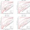 |
Fig. A.1 Hardness ratio diagrams in 0.5–7.3 keV energy band, defined by Barrado et al. (2011), comparing our sample with the stars of the young Collinder 69 cluster (grey crosses). For illustration, error bars corresponding to 0.15, which is the mean error found in the HR estimates of our sample, are plotted in the first panel. Top panels present the sources from fields E (diamonds) and C (squares), while S (triangles) and W (circles) are shown in the bottom. Grids from the APEC model are shown in red, using dotted lines for 6.0 < log T< 8.5 (increasing from left to right, in steps of 0.5). Power-law grid with γ = 0, 1, 2 is shown by black dotted lines (increasing from left to right). Both grids use full lines to represent 20 < log NH< 23, increasing in steps of 0.5, from bottom to top. |
Our analysis was restricted to the sources with estimates in the range − 1 <HR< 1. These limits avoid sources with soft emission at the same level found in the background (HR> 1) and sources lacking of emission in the hard bands (HR< 1). Following Nebot Gómez-Morán et al. (2013), our subsample was also constrained to the sources with HR error bars smaller than 0.3. Among 340 sources with PN data, only 196 sources with HRs in the B2011 bands (Fig. A.1) fulfil these restriction criteria and could be compared with the grids. Among these sources, 133 are only compatible with the APEC grid while 9 are only compatible with the PWL grid. The other 54 coincide with both models. For H2001 HRs diagrams (Fig. A.2) the number of analysed sources is little lower than the subsample studied in the B2011 energy ranges, probably due to intrinsically low emission of stars in the soft band or high absorption of our observations in the soft band (0.2 to 0.4 keV), which gives HR1H2001 = − 1 for several of the sources. In total, Fig. A.2 contains 178 sources, 137 of which are compatible with the APEC grids, 8 for PWL and 33 for both.
Parameters of X-ray flares detected on CMa R1 sources.
Aiming to enlarge the number of classified sources and to solve inconclusive characterization of sources that coincide with the two model grids, we combined the results from both definitions for energy bands. For each source we adopted the more reliable classification that could be found by comparing its position in both Figs. A.1 and A.2. If a given source falls in the models overlapping region of the B2011 HR diagram, for instance, and coincides with the H2001 APEC grid, it is classified as compatible with the APEC model.
We could not discuss the origin of 193 sources because 149 of them have no data available in any HRs diagram and 44 sources remained consistent with both models (APEC and PWL). In total, 194 sources were classified according to their X-ray emission. About 6% (11/194) of these sources are only compatible with the PWL model, so they probably are extragalactic or evolved objects, while 94% (183/194) may have stellar origin.
The HRs of ~60% of the sources are compatible with the APEC model grid. The majority of these sources are found in the ranges 21 < log NH< 22 and 6.5 < log T(K) < 7.5, which corresponds to the plasma temperature expected for low-mass young stars (Feigelson & Montmerle 1999). In spite of their larger scattering, in Fig. A.1 these objects have HRs comparable with the young stars associated with the low extinction stellar cluster Collinder 69, studied by Barrado et al. (2011), which are more concentrated in between log NH = 20–21.5. The results are discussed in Sect. 3.
Aiming to discuss the efficiency of adopting the HRs diagrams to select young star candidates, we compare here the results from Sect. 3.1 with the ages that were determined in Sect. 4.1 and analysed in Sect. 4.3. In this comparison, we consider only X-ray sources with HRs that are inside the diagrams edges and have NIR counterparts with ages well determined (our “best sample”). So that 130 and 134 objects were taken into account in B2011 and H2001 diagrams, respectively.
The histograms in Fig. A.3 show the distribution of number of sources as a function of age compared with their position in the HRs diagrams. As expected, most of the objects, in all the PMS ranges of age, correspond to the APEC (stellar emission) model for both HRs diagrams. Only a few sources (~10%), mainly for B2011 and those with >5 Myr, coincide with PWL model or appear out of both grids. Finally, Fig. A.3 also shows 10% to 20% of objects with <10 Myr coinciding with both models (APEC and PWL), which is confirmed by both HRs diagrams (B2011 and H2001). This is an indication that these sources must be kept as possible young stars.
If we consider that the sources with infrared excess not included in the “best sample”, more than 75% of theses objects are compatible with APEC model in both HRs diagrams, i.e. they may be young stars that are still embedded or have circumstellar disk. Only a few (4%) coincide with PWL model and the remaining sources (20%) are compatible with both grids.
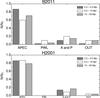 |
Fig. A.3 Distribution of sources coinciding with thermal plasma (APEC) or power-law (PWL) models, and those appearing in the intersection of both grids (A and P) or outside both grids (OUT). |
These results show that our method, based only on X-ray emission, is efficient in identifying young star candidates. In fact, the main difficulty of this method is to obtain the HRs in all soft bands.
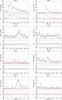 |
Fig. A.4 XMM-Newton EPIC/pn light curves in the energy band 0.5–7.3 keV of X-ray sources with flares. The bottom panels represent the factor |

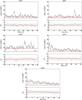 |
Fig. A.5 XMM-Newton EPIC/pn light curves in the energy band 0.5–7.3 keV of X-ray sources with flares and “partial flares”. The bottom panels represent the factor |

Appendix A.2: Flares
The extraction of light curves was made for 340 sources detected with the EPIC-PN camera (typical exposures ~30 ks) in the 0.5–7.3 keV energy band by estimating the count rate in time bins of 1000 s. For each source, the count rate was calculated over an area of the image, the size of which is proportional to the intensity of the X-ray emission. The radius of the extraction region varies from r = 10′′, for faint sources (LX ~ 3 × 1029 erg/s) to r = 40′′ for the brightest source showing flare (LX ~ 4 × 1031 erg/s), but typical values were about 15′′. Following standard routines from SAS13, the background light curve, corresponding to an area of the same size near the source (on the same detector), but free of other sources contamination, was subtracted from the light curve measured at the source position. We searched for sources showing signs of variability by adopting the elevated levels 1.2 × Cch + 1.5σch<Ci< 2.5 × Cch + 1.5σch proposed by Wolk et al. (2005) to indicate peaks of X-ray emission (Ci, in a time bin (i)) detected above the characteristic count rate (Cch ± σch). Thirty-two objects were found showing two or more peaks of intensity. In order to identify variations caused by flares, in a first step we estimated Cch by the linear fit of count rates in the bins (1000 s each) with lowest count rates in a time interval.
We consider a flare-like candidate the event with an increase by factor  higher than 3, where Ci and σi are the count rate and its error in a time interval i, respectively. The flare-like events were confirmed using the definition of flare proposed by Wolk et al. (2005) and Stelzer et al. (2007), which makes use of amplitude (Ai) and the derivative (Δi) of a count rate in a time interval, both defined as
 ![Mathematical equation: \appendix \setcounter{section}{1} \begin{eqnarray} &&A_{i} =\frac{C_{i} - 2\sigma_{i}}{C_{\rm ch} + 2\sigma_{\rm ch}} \label{eq.3.2} \\ &&\Delta_{i+1} =\frac{(C_{i+1} - C{i})/C{i}}{{\rm MIN}[t_{i+1}, t_{i}]}~[{\rm s}^{-1}] \label{eq.3.3} . \end{eqnarray}](/articles/aa/full_html/2018/01/aa30815-17/aa30815-17-eq203.png) The confirmed flares have amplitude Ai> 1.5 in one or more consecutive bins and the maximum derivative in these intervals above the threshold is Δi> 5 × 10⁻⁵. We also derived the flare luminosity Lf subtracting the characteristic luminosity Lch from the average value of source luminosity during the flare. The flare energies (Ef) were calculated by multiplying this Lf by the time interval during which the X-ray emission is larger than Cch.
The confirmed flares have amplitude Ai> 1.5 in one or more consecutive bins and the maximum derivative in these intervals above the threshold is Δi> 5 × 10⁻⁵. We also derived the flare luminosity Lf subtracting the characteristic luminosity Lch from the average value of source luminosity during the flare. The flare energies (Ef) were calculated by multiplying this Lf by the time interval during which the X-ray emission is larger than Cch.
The light curves of the 13 sources with flare-like events are presented in Figs. A.4 and A.5. The increasing factor is shown in the bottom panel of these figures. All parameters derived for these events are listed in Table A.1. Sources E001, E003, and C007 have shown a strong flare. Sources C006 and E041 shown a decay phase that we called “partial” flare, while only the source E007 was not confirmed by Stelzer et al. (2007) criteria.
Spectral parameters of CMa R1 bright sources.
Appendix A.3: Spectra
In order to investigate the X-ray emitting plasma we analysed the low-resolution EPIC spectra integrated over the whole exposure. They were grouped according to the number of counts, adopting a threshold of 10 counts per bin, after background subtraction. We tested fits for the 1T and 2T temperature APEC models. However, owing to intrinsically low luminosity, bad statistics, or quality of spectra, only the 1T model produced good fits with Z = 0.2Z⊙ (see Appendix A.1), and photoelectric absorption model (PHABS) in the XSPEC environment. The fits and the residual [σ(data − model) ×Δ(χ2)] of observed spectra are shown in Fig. A.6. Best-fits parameters were found by χ2 minimization. A good fit with 0.75 <χ2< 1.3 was achieved for only 21 sources. The fit parameters (NH and kT1), reduced χ2 , and degrees of freedom (d.o.f) are presented in Table A.2, along with the derived fluxes (and luminosities) in the 0.5–7.3 keV band.
The hydrogen column density obtained from the spectral fits varies from 0.4 × 1021 cm-2 to 5.4 × 1021 cm-2 with mean value NH = 1.8 ± 1.5 × 1021 cm-2, which corresponds to an extinction AV = 0.9 ± 0.7 mag, adopting NH = 2.1 × 10²¹AV cm2 (e.g. Vuong et al. 2003). The coronal temperatures in Table A.2 vary from 0.7 to 2.1 keV with an average value of 1.4 ± 0.4 keV.
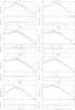 |
Fig. A.6 Best fits and residual (see Sect. A.3) obtained for spectra of bright X-ray sources. |
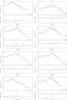 |
Fig. A.6 continued. |
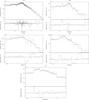 |
Fig. A.6 continued. |
Appendix B: Catalogue of X-ray sources
In this section we present all the 387 X-ray sources detected with EPIC cameras PN, MOS1, and MOS2 in tabular form (Table B.1). The infrared counterparts candidates of these sources (2MASS and WISE) are presented in Table B.2.
X-ray sources detected in the combined images of the EPIC cameras PN, MOS1 and MOS2.
Infrared 2MASS photometry, mass, age, and infrared classification of members of CMa R1 region and counterparts to X-ray sources.
All Tables
Number of X-ray sources as a function of age and mass ranges and their spatial distribution.
X-ray sources detected in the combined images of the EPIC cameras PN, MOS1 and MOS2.
Infrared 2MASS photometry, mass, age, and infrared classification of members of CMa R1 region and counterparts to X-ray sources.
All Figures
|
Fig. 1 Left: spatial distribution of X-ray sources detected by XMM-Newton (fields E, C, S and W; full lines) on the AV map (Cambrésy, priv. comm., 2000) with AV = 2.0 and 4.0 mag contours, compared with ROSAT fields from Gregorio-Hetem et al. (2009; dashed lines). Right: mosaic of images of XMM-Newton EPIC PN, MOS 1, and MOS 2 for the same CMa fields combined in three different energy bands. The red, green, and blue filters present the soft band (0.5–1.0 keV), medium band (1.0–2.0 keV), and hard band (2.0–7.3 keV), respectively. |
| In the text | |
|
Fig. 2 Energy (Ef) and duration (Tf) of X-ray flares on CMa R1 sources (open circles) compared with those observed on members of Taurus molecular cloud (Stelzer et al. 2007), where classical and weak T Tauri are represented by filled circles and squares, respectively. Filled triangles show young stellar objects associated with the η Chamaleontis cluster (López-Santiago et al. 2010). |
| In the text | |
|
Fig. 3 Cumulative distribution of X-ray luminosities for sources in CMa R1 (black lines) and Collinder 69 (Barrado et al. 2011, magenta line). The thick grey line shows the log-normal distribution with μ = 29.3 and σ = 1 proposed by Feigelson et al. (2005). |
| In the text | |
|
Fig. 4 Left: colour–colour diagram for all 340 2MASS counterparts of X-ray sources found in fields E, C, S, and W. Blue symbols represent disk-bearing (Class I and II) stars classified in Sect. 4.2. The ZAMS and locus of giant stars are indicated by thick lines, while the locus of T Tauri stars is represented by a thin line. Dotted and dashed lines show reddening vectors. Right: colour–magnitude diagram showing the isochrones 0.2, 1, 5, 10, 15, 20 Myr, and ZAMS (full lines), early main sequence (grey thick line) and evolutionary pre-MS tracks 0.1, 0.5, 1, 2, 3, 4, 5, 6, and 7 M⊙ (dashed line) from Siess et al. (2000). |
| In the text | |
|
Fig. 5 WISE colours of counterparts of X-ray sources (dots) compared with the locus of Class I and Class II proposed by Koenig & Leisawitz (2014). Open symbols show objects classified according to their infrared excess, while crosses indicate known disk-bearing stars (Fernandes et al. 2015). |
| In the text | |
|
Fig. 6 “Best sample” of X-ray sources based on estimates of masses and ages for 340 2MASS counterparts (see Table B.2). This sample, which takes into account the incompleteness of our sample below ~0.5 M⊙, are present in the grey area. The empty area between dotted lines corresponding to the mass range 0.5–0.7 M⊙ and age >10 Myr is interpreted as the decline of magnetic activity of low-mass young stars with age (see Sect. 7.2). |
| In the text | |
|
Fig. 7 Observed mass distribution indicated by various symbols with error bars. The lines represent the power-law fitting of mass function φ(M) for M> 1M⊙ of individual XMM-Newton fields E (dashed), C (dot dashed), S (long dashed), and W (dotted), and considering the entire “best sample” (black). The grey line shows the theoretical log-normal curve proposed by Chabrier (2005) with μ = 0.3 and σ = 0.6. |
| In the text | |
|
Fig. 8 Comparison of age distributions for each field considering three ranges of age. |
| In the text | |
|
Fig. 9 X-ray fluxes (FX) vs. magnitude in 2MASS J band (mJ). The solid line presents the relationship log (FX) = − 9.8( ± 0.4) − 0,33mJ similar to that obtained using ROSAT data in Paper I. The large symbols represent Herbig Ae/Be stars (M> 2M⊙). Dotted and dashed lines show 1σ and 2σ offset, respectively. |
| In the text | |
|
Fig. 10 X-ray luminosity vs. stellar mass for the sources in CMa R1 (black triangles) compared with T Tauri stars in other star-forming regions: Orion nebula cluster (ONC), Taurus molecular cloud (TMC), and Collinder 69 (Coll69). The dashed line indicates the limit of mass adopted to define our “best sample”. The gap at 0.4–0.5 M⊙ is not real, but due to difficulties in interpolating models on this mass range. |
| In the text | |
|
Fig. 11 Spatial distribution of NIR counterpart of X-ray sources as a function of age. This is compared to a 13CO map10 shown by the grey image superimposed on AV> 2 and 4 mag contours (the same as Fig. 1). The diamonds, squares, and circles represent objects with less than 5 Myr, between 5 and 10 Myr, and more than 10 Myr, respectively. The counterparts found outside of Siess et al. (2000) PMS isochrones are represented by crosses and disk-bearing candidates (see Sect. 4.1) are shown by blue ellipses. Black circles delimit the fields E, C, S, and W. |
| In the text | |
|
Fig. 12 Spatial distribution of NIR counterparts compared with the visual extinction map9. The lowest contours indicate a separation of dense regions (AV> 2). The diamonds and crosses represent XMM-Newton and ROSAT sources, respectively. Top panels a–c show objects with less than 5 Myr, 5 to 10 Myr, and more than 10 Myr, respectively. Bottom panels d–f are objects with masses larger than 2 M⊙, 1 to 2 M⊙ and between 0.5 to 1 M⊙, in this panel are highlighted XMM-Newton objects with masses between 2 and 3 M⊙ (diamonds), 3 and 5 M⊙ (X), and more than 5 M⊙ (full diamonds). Black full lines delimit the fields E, C, S, and W and the ROSAT field is indicated by a dashed line. |
| In the text | |
|
Fig. 13 Same as Fig. 12c (spatial distribution in the age range 10–55 Myr), but for low-mass stars only. In the three panels (a–c), the stellar masses are broken down in three mass ranges (0.5–1 M⊙, 0.5–0.8 M⊙, 0.5–0.7 M⊙, respectively), black diamonds represents XMM-Newton sources, and crosses indicate ROSAT sources. As discussed in the text (Sect. 7.2) and as is visible in Fig. 6, the nearly complete absence of stars with M <0.7 M⊙ is due to the decline of their magnetic activity after ~10 Myr. |
| In the text | |
|
Fig. A.2 Same as Fig. A.1 for hardness ratio diagrams based on 0.2–4.5 keV energy band suggested by Hasinger et al. (2001). |
| In the text | |
|
Fig. A.1 Hardness ratio diagrams in 0.5–7.3 keV energy band, defined by Barrado et al. (2011), comparing our sample with the stars of the young Collinder 69 cluster (grey crosses). For illustration, error bars corresponding to 0.15, which is the mean error found in the HR estimates of our sample, are plotted in the first panel. Top panels present the sources from fields E (diamonds) and C (squares), while S (triangles) and W (circles) are shown in the bottom. Grids from the APEC model are shown in red, using dotted lines for 6.0 < log T< 8.5 (increasing from left to right, in steps of 0.5). Power-law grid with γ = 0, 1, 2 is shown by black dotted lines (increasing from left to right). Both grids use full lines to represent 20 < log NH< 23, increasing in steps of 0.5, from bottom to top. |
| In the text | |
|
Fig. A.3 Distribution of sources coinciding with thermal plasma (APEC) or power-law (PWL) models, and those appearing in the intersection of both grids (A and P) or outside both grids (OUT). |
| In the text | |
|
Fig. A.4 XMM-Newton EPIC/pn light curves in the energy band 0.5–7.3 keV of X-ray sources with flares. The bottom panels represent the factor |
| In the text | |
|
Fig. A.5 XMM-Newton EPIC/pn light curves in the energy band 0.5–7.3 keV of X-ray sources with flares and “partial flares”. The bottom panels represent the factor |
| In the text | |
|
Fig. A.6 Best fits and residual (see Sect. A.3) obtained for spectra of bright X-ray sources. |
| In the text | |
|
Fig. A.6 continued. |
| In the text | |
|
Fig. A.6 continued. |
| In the text | |
Current usage metrics show cumulative count of Article Views (full-text article views including HTML views, PDF and ePub downloads, according to the available data) and Abstracts Views on Vision4Press platform.
Data correspond to usage on the plateform after 2015. The current usage metrics is available 48-96 hours after online publication and is updated daily on week days.
Initial download of the metrics may take a while.