| Issue |
A&A
Volume 609, January 2018
|
|
|---|---|---|
| Article Number | A2 | |
| Number of page(s) | 13 | |
| Section | The Sun | |
| DOI | https://doi.org/10.1051/0004-6361/201730395 | |
| Published online | 22 December 2017 | |
Parametric study on kink instabilities of twisted magnetic flux ropes in the solar atmosphere
1 Centre for Mathematical Plasma Astrophysics, Department of Mathematics, KU Leuven, Celestijnenlaan 200B, 3001 Leuven, Belgium
2 Yunnan Observatories, Chinese Academy of Sciences, Kunming, 650011 Yunnan, PR China
e-mail: This email address is being protected from spambots. You need JavaScript enabled to view it.
3 Division of Atmospheric and Geospace Sciences, Directorate of Geosciences, National Science Foundation, Arlington, 22314 Virginia, USA
4 Center for Astronomical Mega-Science, Chinese Academy of Sciences, 20A Datun Road, Chaoyang District, 100012 Beijing, PR China
Received: 5 January 2017
Accepted: 30 August 2017
Abstract
Aims. Twisted magnetic flux ropes (MFRs) in the solar atmosphere have been researched extensively because of their close connection to many solar eruptive phenomena, such as flares, filaments, and coronal mass ejections (CMEs). In this work, we performed a set of 3D isothermal magnetohydrodynamic (MHD) numerical simulations, which use analytical twisted MFR models and study dynamical processes parametrically inside and around current-carrying twisted loops. We aim to generalize earlier findings by applying finite plasma β conditions.
Methods. Inside the MFR, approximate internal equilibrium is obtained by pressure from gas and toroidal magnetic fields to maintain balance with the poloidal magnetic field. We selected parameter values to isolate best either internal or external kink instability before studying complex evolutions with mixed characteristics. We studied kink instabilities and magnetic reconnection in MFRs with low and high twists.
Results. The curvature of MFRs is responsible for a tire tube force due to its internal plasma pressure, which tends to expand the MFR. The curvature effect of toroidal field inside the MFR leads to a downward movement toward the photosphere. We obtain an approximate internal equilibrium using the opposing characteristics of these two forces. A typical external kink instability totally dominates the evolution of MFR with infinite twist turns. Because of line-tied conditions and the curvature, the central MFR region loses its external equilibrium and erupts outward. We emphasize the possible role of two different kink instabilities during the MFR evolution: internal and external kink. The external kink is due to the violation of the Kruskal-Shafranov condition, while the internal kink requires a safety factor q = 1 surface inside the MFR. We show that in mixed scenarios, where both instabilities compete, complex evolutions occur owing to reconnections around and within the MFR. The S-shaped structures in current distributions appear naturally without invoking flux emergence. Magnetic reconfigurations common to eruptive MFRs and flare loop systems are found in our simulations.
Key words: Sun: filaments, prominences / Sun: flares / magnetic reconnection / instabilities / magnetohydrodynamics (MHD) / Sun: coronal mass ejections (CMEs)
© ESO, 2017
1. Introduction
Research on magnetic flux ropes (MFRs) is critical to understand many complex phenomena on the Sun. Thin flux ropes can be generated by dynamo processes in the convection zone (Parker 1979). When MFRs emerge at the photosphere, sunspots and active regions form and the global coronal magnetic field topology is dominated by loops, which are characterized by arch-like shapes. Convective motions in the photosphere make the loops subject to twist and writhe, and magnetic energy is thus transported and stored in the corona. When the accumulated nonpotential magnetic energy and helicity reaches certain thresholds, magnetohydrodynamic (MHD) instabilities become inevitable and trigger the release of free magnetic energy, which is manifested in various eruptive events, such as flares, jets, filament eruptions, and CMEs.
In solar eruptions, current-carrying helical MFRs are usually inferred from observations (Cheng et al. 2011, 2012; Zhang et al. 2012; Li & Zhang 2013; Yang et al. 2015) and form a core component of various theoretical models (Amari et al. 2003; Fan & Gibson 2004, 2007; Török et al. 2004; Török & Kliem 2005). Highly twisted MFRs in active regions usually mean more free magnetic energy and so these regions are prone to more energetic flares (Maeshiro et al. 2005; LaBonte et al. 2007; Park et al. 2008, 2010; Thalmann & Wiegelmann 2008; Jing et al. 2010; Sun et al. 2012; Tziotziou et al. 2012). It is therefore reasonable to conjecture that a maximum twist exists, above which certain MHD instabilities are inevitable and an eruptive process happens. In reality, the stability of equilibrium states of MFRs are influenced by ambient magnetic topologies, plasma convection in the photosphere, and the detailed MFR internal structure. This complicates the analysis of observational data of an erupting magnetic structure, where one would like to measure the amount of twist and identify whether the eruption is a direct consequence of MHD instabilities.
Over the past two decades, observational knowledge concerning MFRs during explosive events has been continuously accumulating. The helical structure of MFRs has been reported during CMEs with observations by the Large Angle Spectrometric Coronagraph (LASCO) on SOHO (Chen 2011; Vourlidas et al. 2013; Vourlidas 2014). Vourlidas et al. (2013) found that at least 41% of CMEs exhibit clear signatures of an MFR among a large number of CMEs (2403 events). Images obtained with the Yohkoh Soft X-ray Telescope suggest the presence of twisted MFRs (Manoharan et al. 1996; Rust & Kumar 1996; Canfield & Pevtsov 1999; Pevtsov 2002). High-resolution multiwavelength observations from TRACE, SDO/AIA, and Hinode/SXT frequently exhibit helical MFRs associated with eruptive events (Kumar et al. 2011; Zhang et al. 2012; Kumar & Cho 2013; Patsourakos et al. 2013; Cheng et al. 2015).
It is widely accepted that the eruption of twisted flux ropes can be triggered by kink instability (Liu et al. 2007a, 2010; Liu & Alexander 2009; Guo et al. 2012, 2013; Yan et al. 2014, 2015; Török et al. 2004; Gordovskyy et al. 2014; Pinto et al. 2016) or torus instability (Kliem & Török 2006; Fan & Gibson 2007; Fan 2010; Aulanier et al. 2010; Olmedo & Zhang 2010; Savcheva et al. 2012; Zuccarello et al. 2014). Kink instabilities relate primarily to the number of turns on the surface of a MFR or to its internal twist profile, while torus instability depends mostly on the overlying magnetic field variation above the arched loop. The exact number of turns required to trigger a kink instability depends on the geometry of the MFR, the ambient magnetic structure, and the anchoring of this structure in the photosphere; the number of turns may vary because of plasma convection around their footpoints. Vrsnak et al. (1991) found that all prominences with high twists (>2.5π) erupted, while low twist prominences (less than 2π) did not erupt. Rust & Kumar (1996) analyzed 49 transient bright sigmoid structures with their MFR model. They found that the distribution of sigmoids as a function of aspect ratio falls off abruptly below the threshold for kink instability. Guo et al. (2012) calculated the turns of pre-eruptive MFRs and found that the observed number of turns are highly consistent with the thresholds of the kink instability obtained from numerical simulations. Leka et al. (2005) found that some MFRs can carry greater than one turn, which means that the kink instability can serve as a trigger mechanism for solar eruptive events. At least a complete turn for a straight MFR with line-tied effects is needed (Hood & Priest 1979a; Baty et al. 1998; Browning et al. 2008; Bareford et al. 2010).
In addition, there are rare cases in which hard X-ray sources are observed at the footpoints of MFRs (Su et al. 2007; Ji et al. 2008; Jing et al. 2008, 2010; Liu et al. 2007b; Guo et al. 2012; Wang et al. 2015). For example, Liu & Alexander (2009) investigated three kinking filament events with HXR emissions at the footpoints. They proposed that magnetic reconnection occurs as a result of the interactions of two rotating filament legs. Guo et al. (2012) studied extreme ultraviolet (EUV) brightenings that appeared in footpoints of erupting filaments and proposed that internal kink instability may be responsible for the heating inside coronal loops. Yang et al. (2015) reported an X-class circular ribbon flare, in which two HXR sources appeared at both footpoints of the MFR.
To understand eruptive twisted MFRs in the solar atmosphere, MHD kink mode in a cylindrical line tied loop has been studied intensively (Raadu 1972; Hood & Priest 1979b; Einaudi & van Hoven 1983; Velli et al. 1990; Mikic et al. 1990; Longcope & Strauss 1994; Baty & Heyvaerts 1996; Baty et al. 1998; Baty 2001; Galsgaard & Nordlund 1997; Gerrard et al. 2002; Huang et al. 2006, 2010; Browning et al. 2008; Bareford et al. 2010). Hood & Priest (1981, 1979b) computed stability thresholds for the ideal MHD kink mode in coronal loops and showed the stabilising effect of line-tying. Galsgaard & Nordlund (1997) and Lionello et al. (1998) investigated kink instabilities for different magnetic configurations and distinguished two different processes: external kink and internal kink. The behavior of kink instability in the nonlinear regime has been investigated with numerical simulations (Velli et al. 1997; Baty 1997; Baty et al. 1998). These simulations showed that an intense current concentration develops along the whole flux rope. Magnetic reconnection may occur in the vicinity of these current layers to release significant amounts of magnetic energy (Baty 2000). The development of kink instability heavily depends on the magnetic configurations.
Fan & Gibson (2003, 2004) and Török et al. (2004) studied kink instabilities of toroidal MFR models by Titov & Démoulin (1999), referred to as the T&D model hereafter, to consider the effect of curvature. Fan & Gibson (2004) showed that an emerging MFR becomes kink unstable if there is a sufficient amount of twist in the corona. Török et al. (2004) performed zero β simulations in a uniform Alfvén speed atmosphere and found that the growth of the kink mode is slowed down by surrounding magnetic field. Instability onset twists are higher than the typical critical value 3.5π. Török & Kliem (2005) showed the rise profile and the helical shape of a confined filament, which is highly consistent with observations. Kliem & Török (2006) indicated that torus instability of an MFR can happen when the overlying fields decrease with height fast enough.
Many more numerical simulations, based on T&D models or similar magnetic structures, have been conducted to study the instabilities and observational features of eruptive MFRs. For example, Karlicky & Kliem (2010) used numerical simulations based on the T&D model to interpret microwave gyrosynchroton radio emission and hard X-ray sources in a solar flare on 18 April 2001. Terradas et al. (2016) used a weakly twisted T&D model to study Rayleigh-Taylor instabilities in solar prominences along with their morphological features. Sharykin & Kuznetsov (2016) investigated the spatial distribution of the microwave emission generated by accelerated electrons in MFRs. Gordovskyy et al. (2014) and Pinto et al. (2016) studied magnetic reconnection inside eruptive twisted coronal loops, the consequent particle acceleration, and thermal and nonthermal emission.
In this paper, we perform a parametric study of the T&D model based on isothermal MHD simulations with a constant temperature atmosphere. Compared to zero β simulations, the isothermal MHD simulations allow us to study effects due to gas pressure variation. Although full MHD simulations are needed to study the detailed thermodynamic evolution, isothermal simulations are simpler and sufficient to study the internal physical processes of MFRs in finite β conditions during eruption. Using a slightly generalized analytical T&D model, we can systematically study the effect of the twist profile inside the MFRs and the competition between gas and magnetic pressure and tension forces in the dynamics of MFRs. In Sect. 2, analytical formulas for the T&D model are revisited. In Sect. 3, we present details of our simulations. In Sect. 4, three basic physical processes of MFRs are highlighted. In Sect. 5, we give a detailed analysis of dynamical processes due to internal kink instabilities. In Sect. 6, simulations with various numbers of turns, major radii, and ambient atmospheres are given to show the diversity in the evolution of MFRs. Finally, our conclusions are given in the last section.
2. Initial three-dimensional magnetic structure
The T&D model, used by many authors to construct models for solar eruptive events (Török et al. 2004; Török & Kliem 2005), is slightly generalized and adopted in this work. Our generalization allows for internal pressure variation, while maintaining the basic 3D magnetic structure. The whole magnetic structure superposes three parts (Titov & Démoulin 1999). The first part is a MFR, with minor radius a, major radius R, and total toroidal current I uniformly distributed over its circular cross section. The other two parts are a line current I0 and a pair of magnetic charges ± q separated by a distance L, lying on the axis of symmetry of the MFR, buried at z = −d under the photosphere. Only the field above the photosphere at z = 0 has a real physical meaning, while all the subphotospheric fields illustrate the construction of the overall configuration.
Under the assumption of a thin MFR, a ≪ R, the equilibrium of the MFR can be decomposed into internal and external equilibrium (Isenberg et al. 1993; Lin et al. 1998, 2002; Mei & Lin 2008). The external equilibrium has been realised by the background field from a pair of magnetic charges ± q. The outward self-inducted force (or hoop force) due to the MFR curvature is balanced by the confining force from the field of the magnetic charges, 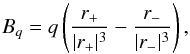 (1)where,
  (2)The vanishing of the total force on the MFR gives a relation between the total toroidal current I of the MFR and the strength q of the magnetic charges,
 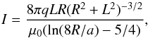 (3)where μ0 is the magnetic permeability in vacuum.
In order to reach a static equilibrium inside the MFR, the inward force from the poloidal magnetic field toward the toroidal axis was balanced by outward pressure, which consists of the thermal pressure of internal plasma and the outward magnetic pressure of the toroidal field introduced by the poloidal current inside the MFR, different from the toroidal field produced by the line current I0. The internal magnetic pressure of the toroidal field can be obtained first from the force-free condition inside the MFR under the assumption of a thin MFR. Next, we replaced part of this internal magnetic pressure by thermal pressure, which allows internal plasma of the MFR to contribute to its internal equilibrium. In doing so, the distribution of thermal plasma pressure can be written as 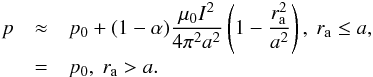 (4)Here,
 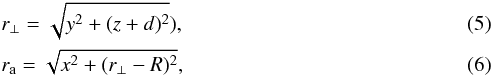 and α is a parameter that controls the contribution of thermal and magnetic pressure on the internal equilibrium of MFR. The constant p0 is the value of the initial uniform pressure outside the MFR. Because of curvature effects, the magnetic tension of toroidal field leads to a downward movement of the line-tied MFR. In contrast, the tire tube force from the internal plasma pressure gives rise to an upward movement (Freidberg 2008). To keep MFRs in equilibrium, the value of α should be adjusted properly for different parameters of the T&D model, such as line current value I0 and minor radius a. Many models in the literature correspond to choosing α = 1, and hence they neglect any internal pressure variation. Our cases refTDa and refTDb, which have α = 1, relate to cases with Φc/π = 4.9 and Φc/π = 2.1 in Török et al. (2004).
The equilibrium between the MFR and the two magnetic charges can lead to an infinite twist on the surface of the MFR because no toroidal field exists outside the MFR. The magnetic field of the line current I0 is included to decrease this to reasonable values, typically less than 4π, suggested by many observations (Liu & Alexander 2009; Wang et al. 2015; Guo et al. 2012). Combining contributions from line current I0 and the poloidal current inside the MFR, the expression for the toroidal field is written as 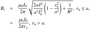 (7)For an analytical expression of the poloidal magnetic field, we follow the practice of Titov & Démoulin (1999), in which poloidal field is given in terms of the vector potential as in
 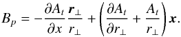 (8)The toroidal At outside the MFR (ρ ≥ a) is
  (9)and inside (ρ<a) is
 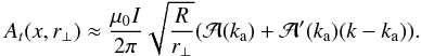 (10)Here,
 ![Mathematical equation: \begin{eqnarray} &&\mathcal{A}(k)=k^{-1}[(2-k^2)K(k)-2E(k)], \\ &&k=2\sqrt{\frac{r_{\perp}R}{(r_{\perp}+R)^2+x^2}}, \\ &&k_{\rm a}=2\sqrt{\frac{r_{\perp}R}{4r_{\perp}R+a^2}}, \end{eqnarray}](/articles/aa/full_html/2018/01/aa30395-17/aa30395-17-eq39.png) and its derivative
and its derivative  (14)These expressions contain the complete elliptic integrals of the first and the second kinds, K(k) and E(k).
Nine sets of parameters for T&D models with different twist turns, embedded in a solar atmosphere with nonuniform β and Alfvén speed.
3. Setup of magnetohydrodynamic simulations
The governing isothermal MHD equations for simulations in this paper are written as ![Mathematical equation: \begin{eqnarray} &&\partial_t \rho +\nabla \cdot (\rho {\vec v}) = 0, \\ & & \partial_t (\rho {\vec v}) +\nabla \cdot \left[\rho {\vec v} {\vec v} +\left(p+\frac {1}{2\mu_0} \vert {\vec B} \vert^2\right)I -\frac{1}{\mu_0} {\vec B} {\vec B}\right] = 0, \\ && \partial_t {\vec B} = \nabla \times ({\vec v} \times {\vec B}). \end{eqnarray}](/articles/aa/full_html/2018/01/aa30395-17/aa30395-17-eq68.png) Here, the conserved variables are the gas density ρ, momentum ρv and magnetic field B. These equations are complemented by the equation of state for isothermal gas, p = cadiabρ. Here, cadiab is a constant, which equals to the squared isothermal sound speed cs. All physical quantities in our simulations are dimensionless with units 5 × 109 cm, 1.28 × 107 cm s-1, 3.89 × 10² s, 1.67 × 10⁻¹⁴ g cm-3, 2.76 Ba, 5.89 G, and 2.95 × 10¹¹ A for length, velocity, time, density, pressure, magnetic field, and current, respectively. Here, these units for density and velocity refer to the initial uniform background atmosphere with electron number density 1010 cm-3, temperature 106 K, and so cs = 1.28 × 107 cm s-1.
Here, the conserved variables are the gas density ρ, momentum ρv and magnetic field B. These equations are complemented by the equation of state for isothermal gas, p = cadiabρ. Here, cadiab is a constant, which equals to the squared isothermal sound speed cs. All physical quantities in our simulations are dimensionless with units 5 × 109 cm, 1.28 × 107 cm s-1, 3.89 × 10² s, 1.67 × 10⁻¹⁴ g cm-3, 2.76 Ba, 5.89 G, and 2.95 × 10¹¹ A for length, velocity, time, density, pressure, magnetic field, and current, respectively. Here, these units for density and velocity refer to the initial uniform background atmosphere with electron number density 1010 cm-3, temperature 106 K, and so cs = 1.28 × 107 cm s-1.
These equations have been solved by the MPI-parallelized Adaptive Mesh Refinement code (MPI-AMRVAC) (Keppens et al. 2012; Porth et al. 2014). This code consists of several independent modules to advance hyperbolic partial differential equations with various numerical schemes. The numerical schemes used in this work are a third-order accurate, shock-capturing finite volume spatial discretization, which combines a Harten-Lax-van Leer approximate Riemann solver (Harten et al. 1983); a third-order limited flux reconstruction (Čada & Torrilhon 2009); and a three-step Runge-Kutta time marching method.
The computational domain is a 3D uniform box of sizes −4 ≤ x ≤ 4, −4 ≤ y ≤ 4, and 0 ≤ z ≤ 8 in Cartesian coordinates, and 2003 grid points are typically employed. For MFRs with minor radius a = 0.65, there are 33 grid cells in the radial direction to resolve internal processes inside the MFRs. At the bottom of the simulation box is a line-tied boundary to simulate the photosphere environment, where footpoints of magnetic field lines are anchored into slowly moving dense plasma. Line-tied conditions are realized by fixing all three components of velocity at z = 0 to zero and keeping the magnetic field in the ghost cells unchanged during the simulation. For the other five boundaries, we adopted open boundary conditions, in which ghost cells of all physical variables come from extrapolation of nearby internal grid cells. Because we put emphasis on the internal physical process of eruptive MFRs in this parametric study, more complex boundaries are not necessary for the problems we addressed.
Our simulations use the pressure-generalized T&D model discussed in the previous section, with nine sets of parameters shown in Table 1, which are divided into three groups for different purposes. In all cases, parameters related to the shape of MFR R, d, and L have been fixed to 2.2, 1, and 1, respectively. The strength of magnetic charges q is fixed to 27.2, and so the total toroidal current I inside MFRs is fixed to 3.6 because of the requirement of external equilibrium. In addition, the value of p0 and cadiab are also fixed to 1. We adjust the line current I0 to get different twist turns, α and atmosphere density ρ to obtain different plasma β, and minor radius a to get different geometries of MFR.
 |
Fig. 1 Initial magnetic configuration for case refTDb. Colored curves with green indicate internal MFR field lines, orange indicates the boundary MFR, and blue indicates the surrounding; the distribution of normal magnetic field (red-green shadings) on the bottom plane z = 0 and a black line denotes the magnetic axis of MFR. The translucent isosurface of current is for j = 0.4jmax, which is used also for all current isosurfaces in the following. Here, jmax is the maximum current value inside the initial MFR. The units in this plot and all the following plots are dimensionless with conversions as given in Sect. 2. |
As an example, the initial magnetic structure of case refTDb, which is one parameter set in Table 1, is given in Fig. 1. In this case, the line current I0 is equal to −9.5 and the minor radius a is equal to 0.65, so that average values of the normal magnetic component around the MFR and on the bottom of the simulation box is up to 40 G. The magnetic field lines inside, outside, and on the MFR surface are illustrated by green, blue, and orange curves, respectively; the MFR is shown as a gray isosurface j = 0.4 jmax. Here, jmax is the maximum current value inside the initial MFR. A black line inside the gray surface is the magnetic axis, where the poloidal magnetic field vanishes. The detailed distribution of physical variables along the cut on the z-axis is given in Fig. 2. Specifically, we measure the twist turns distribution by two different methods: an analytical formula from the definition of turns for a straight MFR and a numerical method that counts the turns of magnetic lines around the MFR magnetic axis.
The twist turns Φ(r) for a straight MFR with length 2πR has been defined as  (18)Here, r is the distance away from the axis of a straight MFR with uniform internal current distribution. However, as our MFR is curved and anchored to the dense photosphere, only the length of the MFR in the corona (z> 0) must be accounted for. Thus, twist turns in our models are better quantified from
  (19)In panel b of Fig. 2, the black solid line gives twist turns distribution Φc along the z-axis. Furthermore, we obtain the distribution of the safety factor q along the z-axis, which is the inverse of Φc, widely used to study instabilities in tokamaks, but where q is really quantified as a function of the nested flux surface label.
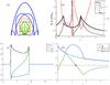 |
Fig. 2 More details about the initial magnetic structure of refTDb shown in Fig. 1. Panel a: magnetic field lines of the configuration in Fig. 1 projected on zx-plane. Panel b: twist turns of magnetic field lines obtained by different methods; the solid black line indicates Φc calculated by Eq. (19), the crosses indicate numerical turns Φnum by integrating the magnetic field around the MFR magnetic axis, and the thick black line indicates the straight flux rope Φcs based on Eq. (20). The red line represents the distribution of the safety factor q = 1/Φc. Panel c: internal toroidal (blue), poloidal (green), and total current (black) distribution of the MFR along the z-axis. Panel d: internal toroidal for α = 1 (blue) and α = 0 (blue dashed), and the poloidal (green) magnetic field strength of the MFR along the z-axis; a cross and a circle indicate the position of the magnetic axis and geometry axis of the MFR, which indicates a Shafranov shift. |
The black thick line in panel b shows the turns distribution of a straight MFR with uniform current profile and length 2Rcos-1(d/R), which is along the y-axis and passes through the point (0,0,R−d). The corresponding equation for this curve is derived by substituting Eq. (7) and the formula of poloidal field for a straight MFR into Eq. (19) as follows:  (20)This curve shows that the twist profile reaches its maximum 1.749 on the surface of MFR, and decreases monotonically with distance away from the MFR surface, and on the z-axis, there exist two points inside the MFR with Φc = 1. By comparing these two curves, we notice that the Shafranov shift of MFR in our models leads to singularities in the black solid line, which confirms that in reality a formula of turns should be based on magnetic surfaces, which is standard practice in tokamak physics.
Hence, more reliable numerical turns Φnum are calculated by sampling points on the z-axis and calculating turns of magnetic field lines passing through those points. The turns for each line is derived by integration of the angle variance along the magnetic axis curve of MFR (Berger & Prior 2006; Guo et al. 2013). As shown in panel b, twist turns from the two methods confirm each other approximately, except near the singularities. In addition, the averaged numerical Φnum is slightly smaller than the analytical averaged  . This is because of the limited numerical resolution in our simulation. These two values become closer if higher numerical resolutions are used to resolve the twist structure inside the MFR.
More details about the toroidal, poloidal, and total current distribution are given in panel c of Fig. 2, and the magnetic field strength for toroidal and poloidal components are given in panel d. When α equals to 1, the toroidal and poloidal magnetic field balance each other to reach the internal equilibrium of the MFR. The poloidal magnetic field of the line-tied MFR moves upward because of curvature. Two magnetic charges are introduced to confine the poloidal field of MFR, so that the MFR reaches its external equilibrium. However, the curvature of toroidal magnetic field inside MFR has not been discussed in detail in previous studies. The tension of internal toroidal field leads to a downward movement of the line-tied MFR, which is discussed in the following.
4. Basic processes related to stability of magnetic flux rope
The T&D model can be used to initiate simulations of the evolution of MFRs and the flux rope embedded solar prominences and filaments, in which the plasma is denser and the temperature is lower than the ambient corona. Our models have constant temperatures by construction, but contain denser plasma when α is less than 1. Similar to a configuration of a circular cross-section tokamak, the MFR curvature implies a competition between three forces, i.e., the hoop force of the poloidal field, the tire tube force, and the 1 /R force (Freidberg 2008). The hoop force relates to outward expansion in that the current runs toroidally (or poloidal magnetic field). The tire tube force exists because plasma pressure in a toroidal tube expands its major radius. The plasma pressure has its contribution on the internal equilibrium when α ≠ 1 in our MFR models (and also for realistic solar prominences in MFRs), and so the tire tube force of internal plasma competes against curvature effects. The 1 /R force comes from a 1 /R dependence of internal toroidal field. The internal toroidal field close to the axis of symmetry of MFR is larger than the part away from the symmetry axis, which leads to a net outward force.
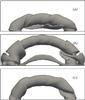 |
Fig. 3 Evolution snapshots of MFRs for cases refTDa, htirep, and ltirep at t = 2.4, 1.5, and 1.5, respectively. The Alfvén time τa for these cases equals to 0.21, as shown in Table 1. The geometry of MFRs is shown by the gray current isosurfaces. Panel a: in case refTDa with α = 1, the MFR crashes downward to the photosphere. Panel b: in case htirep with α = 0, no kink happens, but only an expansion occurs. Panel c: in case ltirep with α = 0.9, internal gas pressure balances the toroidal curvature effect at the early stage of this simulation. |
In order to study the effects of the curvature, we performed three simulations (the cases refTDa, htirep, and ltirep), in which the contribution of plasma pressure to the internal equilibrium quantified by α of MFR is equal to 1, 0, and 0.9, respectively. The evolution of MFRs at the early stage of these simulations is shown in Fig. 3. Without the contribution from internal gas pressure variation, the approximate force-free MFR refTDa crashes downward and eventually hits the photosphere. This is contrary to the situation of a circular cross-section tokamak, where the 1 /R force leads to a movement away from the symmetry axis. As shown in panel a of Fig. 3, because of the curvature, the magnetic tension of the internal toroidal field gives a force toward the symmetry axis of the MFR. For the T&D model, the effect of 1 /R force is partially prevented by the line-tying, while globally the MFR is confined by the background magnetic field from the line current I0 and two magnetic charges ± q. In the line-tied T&D model, the MFR moves downward to the photosphere because of magnetic tension.
In contrast, panel b gives a snapshot for case htirep, α = 0, in which only plasma pressure is used to achieve internal MFR equilibrium. The tire tube force effect of internal plasma expands the MFR in all directions, except at the fixed footpoints of the MFR on the photosphere. Because internal gas pressure is comparable to the internal inward force from the poloidal field of MFR, the averaged value of β inside the MFR is about 5. But β outside the MFR is much lower, about 0.08, as listed in Table 1. The tire tube force of the gas inside the MFR can destroy its equilibrium and give rise to a dynamical eruption in the low β exterior, where the upward velocity of the MFR apex reaches up close to 0.65 times the sound speed cs.
In the case ltirep shown in panel c, a mixed total pressure, with contributions from both internal gas pressure and the internal toroidal magnetic field, is used to achieve the MFR equilibrium. We found that at α close to 0.9, the tire tube force of internal plasma and the curvature effect of toroidal field approximately cancel each other. The MFR can retain its initial structure for enough time until a confined kink instability occurs and develops into its nonlinear stage. There are several factors that make this nonlinear stage very complicated. These factors include the twist profile, curvature effects, confining effects of the ambient magnetic structure, nonperfect internal equilibrium, photosphere line-tied conditions, and surrounding realistic β environment.
 |
Fig. 4 Evolution snapshots of case lowtwist at t = 16.2. The current isosurfaces on the left show the MFR geometry for different viewpoints. The current distribution on the right shows the internal MFR structure on the cut plane y = 0. |
Among these factors, the twist turns play a critical role in the complex evolution of MFR. To demonstrate this, we performed another two extreme cases, lowtwist and inftwist, to study simpler situations. Parameters of these two cases are given in Table 1. In case lowtwist, the averaged twist turns and turns on the surface of MFR are lower than 1. As expected from linear theory of kink instabilities, the MFR does not experience a kink instability, and reaches a numerical equilibrium state, as shown in Fig. 4. The external geometry shape of the current isosurface of MFR does not obviously change, and the background magnetic field is disturbed slightly around the MFR. However, a slow redistribution process of current occurs inside the MFR, although there exists an approximate balance between inward force from poloidal magnetic field of MFR and mixed pressure. A current sheet (CS) forms inside the MFR during this current redistribution process.
In another extreme situation, case inftwist, the background field due to the line current is removed. The twist on the surface of this MFR is infinite because of the vanishing of the toroidal field on that surface. Beside the curvature effect of MFR, which is compensated by internal mixing pressure and the effect of the two monopoles ± q, the magnetic field of MFR has similar structure to a cylindrical z-pinch, which is unstable to kink mode instabilities. The evolution snapshots given in Fig. 5 show that the kink instability dominates the evolution immediately. The geometrical shape evolves from an arch shape into a rectangle shape because of the helical deformation due to kink instability and the line-tied effect at the photosphere. Meanwhile, the central part of the MFR moves upward continuously (Roussev et al. 2003). Similar to 2D analytical flux-rope models (Lin et al. 1998; Lin & Forbes 2000; Mei & Lin 2008; Mei et al. 2012a,b), the central part of the MFR experiences an equilibrium loss process. When the central MFR erupts upward, a CS forms under the MFR and grows in length continuously, wherein magnetic reconnection takes place. According to the theory of Sweet-Parker reconnection, we can estimate numerical diffusion ηnum = vinδ ≈ 0.022, which is also a reasonable estimation for other cases. Here vin ≈ 0.22 is the reconnection inflow and δ ≈ 0.1 is the full width of the CS. The numerical diffusion time τnum = ηnumd2 ≈ 0.05τa. Here, d = 1 represents the characteristic length of the magnetic structure and τa is given in Table 1.
According to the linear theory of MHD instabilities for cylindrical plasma columns (or straight tokamaks), an external kink instability can occur in a plasma-vacuum setup. When twist turns on the surface exceed the Kruskal-Shafranov condition, i.e., the safety factor q< 1 for cylindrical plasma, m = n = 1 external kink instability occurs. Here, m and n are the integer poloidal and toroidal mode numbers, respectively. In case inftwist, there exists a gradient in pressure from internal to outside because we set α = 0.96 in this case. The MFR surface can be treated as an interface between two atmospheres with different thermal pressure. The evolution of MFR is similar to an external kink instability of a cylinder plasma column in the beginning, but evolves into an equilibrium loss process, suggested by 2D flux-rope models. In addition, a kink mode is called external if the resultant perturbation affects magnetized plasma away from its originating site. Based on this, we refer to the instability at the early stage of case inftwist as an external kink instability.
The resultant magnetic structure from internal current redistribution and external kink instability are given in Fig. 6. In panel a for case lowtwist, the magnetic field lines inside the MFR are shown by green lines, the magnetic field overlying the neutral lines are indicated by orange lines, and other undisturbed ambient field lines are shown by blue curves. During internal current redistribution, a CS forms inside the MFR and its lower tip moves downward slightly. From an observational viewpoint, the reconnected loops underneath the CS has a topology similar to the standard flare model scenario, where observed flaring loops may related to chromospheric evaporation scenarios (a process not included in our isothermal simulations; Forbes 2003); the lower tip of the CS connects to the top of a flare loop system, which is identified as a separatrix separating the flare loops from the ambient magnetic field. When the lower tip of the CS moves down, the separatrix of the flare loops move downward along with the apex of the flare loops.
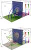 |
Fig. 6 Evolution snapshots of case lowtwist (from Fig. 4) and inftwist (from Fig. 5) at t = 16.2 and 8.4, respectively. The magnetic field structures are illustrated by colored 3D curves. The blue lines represent the undisturbed magnetic field, orange lines are relative to the CS, and green lines pass nearby the magnetic axis of MFRs. Vertical cuts give the current distributions; horizontal cuts on the bottom give the distributions of normal magnetic field. The thick black lines indicate neutral lines that separate the photosphere plane z = 0 into two areas with opposite normal magnetic fields. |
Panel b shows the magnetic structure of case inftwist. Because of external kink instability, the center part of MFR loses its external equilibrium and erupts upward. Under the MFR, a CS appears that is almost attached to the photosphere and later grows continuously. The low and upper tips of this CS move upward simultaneously, while it remains elongated in the z direction. In the early stage of eruption, there is no flare loops system. Then the magnetic reconnection operates in the CS. Magnetic field lines move into the CS from both sides and come out as reconnected magnetic lines via two tips. This process ensures the continuous upward movement of the MFR, the lower tip of the CS detaches from the photosphere and this leads to growth of the flare loops system.
The behavior of the flare loops system in cases lowtwist and inftwist are significantly different. In case lowtwist, the magnetic field lines overlying the neutral line (thick black lines in Fig. 6) are sheared slightly, and the apex of the flare loops system moves downward. In case inftwist, the magnetic field lines around the MFR and nearby the neutral line are strongly sheared, and the apex of flare loops system move upward continuously during the MFR eruption. Because these two cases represent two extreme situations, the flare loops system in realistic solar eruptions may have features of both cases.
 |
Fig. 7 Time evolution of MFR heights for five cases. The gray line indicates a movement at the sound speed cs. |
In addition, Fig. 7 gives the time evolutions of the heights of MFRs. The heights quantify the z-axis coordinate of the crossing points between the y = 0 plane and the magnetic axis, where the poloidal field vanishes. As shown in this figure, the tire tube force in case htirep shows the fastest upward movement with a speed about 0.65cs. At the other extreme, without the tire tube force, the MFR in case refTDa cannot be stable and a downward crash process occurs because of the downward magnetic tension of toroidal field inside the MFR. This process lasts about 20τa until it hits the photosphere with τa given in Table 1. By adopting a mixed pressure, the MFR in case ltirep remains in approximate equilibrium at the early stage of the simulation. Later, kink instabilities dominate its evolution and lead to a slowly upward movement at about 0.3cs. In case lowtwist, a very slow current redistribution occurs inside the MFR, which leads to a slight upward shifting of the MFR magnetic axis. In case inftwist, the MFR does not move upward quickly in the beginning, but gets distorted into a helical shape. Later, the central part of MFR loses its equilibrium and moves upward with a speed about 0.5cs.
5. Internal kink instabilities
The investigation of eruptive MFRs immediately becomes complex when we move to more general cases. Groups 2 and 3 shown in Table 1 give a parametric study for the complicated kink instabilities of MFR. In case refTDb with a larger radius a than case refTDa, the internal equilibrium of MFR comes from the balance between internal toroidal and poloidal magnetic field. In contrast to refTDa, the enlarged MFR no longer instantly gets pulled down and the curvature effect of toroidal magnetic field is no longer obvious for the MFR with larger minor radius a. We also include a case with α ≠ 1, which is case intkink, where the curvature effect of the toroidal magnetic field is significant. We introduce the tire tube force to cancel this curvature effect by setting α = 0.9.
In this section, we focus on the evolution of these two cases, which are characterized by internal kink instabilities. Figure 8 shows the initial distribution of twist turns along the z-axis for cases in group 2. For both cases refTDb and intkink, curves in Fig. 8 indicate the existence of a q = 1 isosurface inside the MFR, here quantified by the more exact numerical turns Φnum. According to linear theory of internal kink instability for cylindrical plasma (Goedbloed et al. 2010), an m = 1 internal kink is expected to operate at a q = 1 surface.
However, the line-tied condition on the photosphere and the curvature of MFR have significant effect on the evolution of internal kink instabilities. The behavior of the MFR becomes more complex than in the situation of cylindrical plasma. Figure 9 presents evolution snapshots of current isosurfaces in cases refTDb and intkink, which demonstrate complicated MFR dynamics. A set of magnetic field lines, passing through discrete points on the z-axis, illustrate the evolution of magnetic field lines. The magnetic connections inside and surrounding the MFR do not show obvious changes during internal kinks. The current isosurfaces give more details than the magnetic field lines, directly showing redistribution of nonpotential magnetic energy stored in magnetic structures surrounding the MFR.
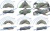 |
Fig. 9 Evolution snapshots of cases refTDb (top row a) and intkink (bottom row b). The colored curves represent the magnetic field lines outside (blue and orange) and inside (green) the MFR. Translucent isosurfaces indicate the current structures of the MFR. |
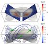 |
Fig. 10 Rotational movement in case refTDb. Panel a: current distributions on two cuts of MFR at t = 5.4, and the current isosurfaces give the geometry shape of MFRs. Panel b: velocity distribution on two cuts; the three green arrows indicate the direction of rotation. The curves show the magnetic field lines passing through discrete points on the z-axis. |
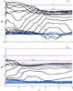 |
Fig. 11 Disturbances in By as function of time at discrete points on the z-axis for case refTDb (panel a) and case intkink (panel b). The labels on curves are the z-axis coordinate of the sampled points. Sample points below/above the MFR are colored blue/purple. |
Further analyses of the internal kink instability in case refTDb are shown in Figs. 10 and 11a. Figure 10 shows the resultant rotational movement of plasma around the MFR. The current iso-surfaces in two panels of Fig. 10 give the geometric structure of MFR. The current and velocity distributions on two cuts of the MFR show the internal current structures and plasma rotational movement around the MFR, respectively. In panel 10a, the current distribution on the cuts show the helical distortion due to the internal kink instabilities. The current distribution evolves into two parts: a helical current ribbon and a CS located at the lower part of the MFR. This helical current ribbon is not in equilibrium and will move upward slightly. Later overlying magnetic field from I0 and ± q prevents its upward motion. In panel 10b, the directions and values of velocity of rotating plasma are shown by the colored arrows, and the magnetic field lines passing through discrete points on the z-axis are given by curves. The values of plasma velocity field around the MFR is subsonic with the exception of a small region under the MFR, and the direction of the velocity field shows simultaneous downward and upward flow, which is consistent with the red- and blueshifts observed in synthetic Doppler map generated from a 3D simulation of a kinked straight MFR (Pinto et al. 2016; Snow et al. 2017). In addition, the rotations on left and right regions of the MFR are anticlockwise when we look downward from above. On the other hand, the left rotation is clockwise and the right rotation is anticlockwise when we look from left side. The green arrows in panel b indicate the overall rotation direction around the MFR, which is typical for a helical distortion. Because of rotation movement, the magnetic field lines around the MFR experience an anticlockwise shearing process when we look downward from above.
Figure 11a gives the changes of By on z-axis positions over time, which illustrates the disturbance of background magnetic field by the internal kink instabilities. Each curve gives the evolution of By at 1 of 20 points, uniformly distributed on the z-axis from 0 to 3.6. The blue and purple curves indicate points relatively far away from the MFR. As shown by these blue and purple curves, the dynamical evolution by internal kink is confined to a small region around the MFR. Because the magnetic structure in our work is significantly different from a cylindrical MFR or tokamak, the internal kink also slightly affects regions outside the MFR surface. In principle, this instability is confined inside the MFR boundary, and there is no perturbation on the external environment (Baty 2000, 2001). Considering the inevitable influence from the line-tied condition and the curvature of MFR, we conclude that eruptive processes in case refTDb have typical characteristics of internal kink instability.
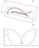 |
Fig. 12 Panel a: colored magnetic field lines whose start points are on the left (green) and right (purple) foot points of MFR at t = 5.4. The red arch represents the initial magnetic axis. Panel b: trajectory of crossing points between the panel y = 0 and magnetic field lines. |
Connection changes in magnetic field lines inside the MFR are illustrated in Fig. 12. The purple and green magnetic field lines are obtained by tracing from the left and right footpoints of the initial magnetic axis location, respectively. The trajectory of their cross points, where they intersect the plane y = 0 as time progresses, are shown in panel b. From these trajectories, we can see that the magnetic field lines and the plasma movements shown in Fig. 10 have the same rotational direction. The helical deformation of MFR leads to topology changes in which the magnetic line defining the initial magnetic axis separates into two magnetic field lines that gradually separate after the beginning of our simulation. This implies that magnetic reconnection occurs inside the MFR.
For case intkink, the internal kink instability also dominates the evolution of MFR. The evolution snapshots for this case are given in Fig. 9b. As in case refTDb, internal kink instability leads to dynamical current redistribution inside the MFR and rotating plasma around the MFR. Similar to case refTDb, the dynamical evolution remains largely confined inside the MFR and the surrounding magnetic field lines have been slightly disturbed. Figure 11b shows the disturbances outside the MFR by internal kink, which indicates the changes of By over time at 20 points, uniformly distributed on the z-axis from 0 to 3.6. The blue and purple curves confirm that the dynamical processes of internal kink is confined inside. The connections of magnetic field lines have been changed in case intkink as well, pointing to magnetic reconnection processes inside the MFRs. In addition, we also performed two higher resolution simulations with 3003 grid points for cases refTDb and intkink to evaluate the effect of the numerical resolution on the evolution of the internal kink. The main characteristics of the evolution processes described above remains unchanged.
6. Mixed kink instabilities scenarios
In this section, another set of T&D models (see group 3 in Table 1) are investigated to demonstrate more complex features of kink instabilities of MFRs. Similar to cases in group 2, we introduce the internal tire tube force to compensate for the curvature effects of toroidal components approximately by setting α = 0.8 for case mixa and 0.9 for case mixb. In addition, we also mention case ltirep in group 1. Previously, we stressed the internal equilibrium at the very early stage in case ltirep as shown Figs. 3c and 7.
In comparison with cases in group 2, the cases mixa, mixb, and ltirep have higher twist turns. The averaged twist turns and the turns on the surface of the MFR shown in Table 1 exceed Kruskal-Shafranov limits, and hence the external kink instability dominates the evolution of MFRs. Figure 13 gives the initial distribution of twist turns along the z-axis for these cases. The twist turns reach their maximum on the surface of MFR. Similar to cases in group 2, q = 1 surfaces also exists inside the MFR for all cases in group 3. Thus, the internal kink instability may play an important role in the dynamical evolution of these MFRs as well.
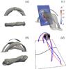 |
Fig. 14 Panels a, b: evolution snapshots of MFR for case mixa shown by current isosurfaces from different viewpoints at time t = 2 and 9.6. Panel c: current distribution snapshot on chosen cuts at same time as panel b. Panel d: flux function of poloidal field At on the cut y = 0, and magnetic field lines (blue) rotating around different magnetic axes (red). |
Figure 14a and b shows evolution snapshots of case mixa. In the early stages, the MFRs twist into helical shape because the turns exceed the Kruskal-Shafranov limit. A strong rotating velocity field forms around the MFR, and this MFR evolves into two independent MFRs with a CS connecting both of these MFR. Panel c shows the resultant internal current distribution; and panel d confirms the existence of two newly formed MFRs. Two axes of MFRs are formed that are illustrated by the red curves, and two magnetic field lines (blues) are shown to rotate around these two different axes. Furthermore, the black contours of magnetic potential At for poloidal magnetic field on the plane y = 0 confirms the formation of two independent MFRs.
In addition, unlike the external kink instability in case inftwist, the evolution of case mixa has been suppressed by the strong background field from the line current I0. Helical distortion does not lead to a loss of external equilibrium and the MFR almost stays at its initial position. Thus, this case has more characteristics of the internal kink instability, as is also shown in cases refTDb and intkink.
 |
Fig. 15 Panels a, b and c: same as Fig. 14, but for case mixb at t = 3.6 and 15. Panel d: magnetic field lines around the footpoints of MFR (blue) and along the CS (orange). |
For the case mixb, the evolution snapshots are given in Fig. 15. The MFR twists itself into a helical shape immediately. Later, the central part loses its external equilibrium, moves upward and so lifts the whole MFR upward. When the upward-moving MFR collides with the overlying background field, a helical CS forms surrounding the MFR. This confines the further eruption of the MFR. In comparing the disturbed region of background field and atmosphere in cases refTDb, intkink and mixa, the disturbed region in case mixb is obviously larger. This is because the kink instability in case mixb has characteristics of external kink instability. Dynamical evolutions of cases inftwist and mixb have the same physical cause, i.e., the violation of the Kruskal-Shafranov condition.
On the other hand, the external kink instability does not dominate the evolution of this case mixb since this process is suppressed by the overlying background field. Other physical factors have significant effects on the evolution of MFR. First, the q = 1 surface inside the MFR leads to internal kink instability inevitably. Then, the helical distortion of MFR breaks internal equilibrium, which involves the fragile balance among the poloidal and toroidal magnetic fields and the tire tube force of gas.
As shown in Fig. 15c, the initial helical MFR experiences dynamical current redistribution and evolves into a helical current ribbon, as a result of internal equilibrium loss. A CS under the helical current ribbon forms during the evolution. Its formation involves internal current redistribution and the converging movement of magnetic field lines on both sides of the CS when the MFR moves upward. We find analogies with the formation of CS in the 2D flux-rope model (e.g., see Forbes & Lin 2000; Lin & Forbes 2000; Lin et al. 2002; Mei & Lin 2008; Mei et al. 2012a,b, for more details). Based on these findings, we can refer to the dynamical evolution of case mixb as resulting from a mixed kink instability. Furthermore, Fig. 15d shows a close relationship between the CS and a sigmoid structure, which is a very common structure in active regions of the solar atmosphere. In the center of the sigmoid structure, the orange magnetic field lines divide two different connectivity regions on the photosphere. Along these magnetic field lines, a 3D CS exists. On both sides of the CS, there is a pair of magnetic field lines that together compose an S-shape.
Our last example for the mixed kink instability is case ltirep, where we investigate the evolution of a MFR with higher twist turns and smaller minor radius than in case mixb. The early evolution of this case has already been discussed in Sect. 4, and the changes of MFR height with time are given in Fig. 7. Similar to case mixb, the MFR is distorted and then loses its external equilibrium, moves upward, collides with overlying background magnetic field, and a helical CS surrounds the MFR. Meanwhile, the fragile internal equilibrium is broken, a CS forms under the MFR and a sigmoid structure appears. The whole evolution is very complex, so that it is very hard to distinguish one physical effect from others. Basically, this evolution involves a highly distorted MFR, whose complexity compares with the MFR given by Archontis & Hood (2008).
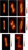 |
Fig. 16 Evolution snapshots of ∫ | j | dz for case mixb (a) and ltirep (b), in which the S-shaped sigmoidal structures form and surround the original MFRs. Panels c and d: evolution snapshots of ∫ | j | dz for cases intkink and infkink to show more possible geometrical features of MFRs. |
To conclude, we present snapshots of helically distorted MFRs in Fig. 16, which allow us to make a direct comparison with observational sigmoid structures. This figure gives distributions of ∫ | j | dz, the integration of | j | along the z-axis, for cases mixb (panel a) and ltirep (panel b) at different times. These integrated current distributions show that the S-shaped sigmoid structures form during the mixed kink instabilities in both cases. These sigmoids also appear in the numerical experiment by Roussev et al. (2012), where an S-shape structure was the result of a flux emergence process. In case mixb, for example, panel a in Fig. 16 indicates that the original MFR evolves into a CS and a pair of new MFRs at t = 15, whose corresponding 3D structures are shown in Fig. 15. Each new MFR inherits one footpoint from the original MFR, which is fixed to the photosphere. Another part of each MFR is actually free floating in the corona. At t = 15, the distribution of ∫ | j | dz does not display a clear S-shape structure yet. After further evolution, the free-moving areas of new MFRs grow and surround the footpoints of the original MFR, and these two MFRs and the CS in the center compose the S-shape structure. In addition, another two snapshots of ∫ | j | dz show geometrical changes of MFRs for cases intkink and infkink. In panel c, no S-shaped structure forms during the internal kink process. Only some internal structure of MFR due to current redistribution can be seen. In panel d, the MFR was twisted seriously during the external kink instability. An S-shaped structure forms around the footpoints of original MFR and a CS appears between the footpoints, as shown in Fig. 5. The comparison of these cases in Fig. 16 indicates that the formation of an S-shape structure highly depends on the initial twist profile of MFR.
7. Conclusions
In this work, we studied the parametrically kink instabilities of twisted MFRs in finite β solar atmospheres by performing a set of 3D isothermal MHD simulations. Our main results are as follows.
We performed five simulations to identify the role of three basic concepts, i.e., the tire tube force from finite internal pressure, the possibility of internal current redistribution, and the role of external kink instability. The tire gas pressure inside the MFR is due to the curvature of the MFR and results in an upward expansion. Current redistribution appears inside an MFR, even if twist turns on the surface are less than 1. In order to realize the internal equilibrium, the internal gas pressure and internal magnetic pressure of toroidal field should be combined. Our parameter α controls the two pressures, so that the curvature effects of both cancel each other. However, this strategy only gives an approximate internal balance of MFR, in which a slow current redistribution still occurs. The external kink instability was demonstrated in the evolution of MFRs with infinite twist turns. Owing to the curvature and line-tied photosphere environment, the MFR is distorted into a helical shape and its center region loses external equilibrium and erupts upward continuously.
We carried out simulations of a MFR with low twist to investigate the internal kink instability because of the q = 1 surface inside the MFR. Internal instability distorts the MFRs into helical shape, modifies the current distribution, and leads to rotating velocity fields and the formation of helical CS surrounding the MFRs. Because of the curvature and the line-tied condition, the nonlinear evolution of internal kinks is not confined inside the MFR exactly, and atmosphere and magnetic field in the vicinity of MFRs are slightly disturbed. The helical distortion of MFRs also changes the connection of magnetic field lines.
Next, the evolutions of three MFRs with high twist turns have been studied. In these cases, the high twist turns lead to very complicated evolutions of MFRs, so that it is hard to distinguish physical cause and effect. Because the twist turns exceed Kruskal-Shafranov limits and the existence of q = 1 surface inside the MFR, the dynamical evolutions have characteristics of both external and internal kink instabilities. Thus, we refer to such cases as caused by a mixed kink instability. During evolutions of the mixed kink, a 3D CS forms gradually because of both internal current redistribution and convergence of magnetic fields on both sides of the CS. In addition, an S-shape magnetic structure surrounds this CS. This suggests that the mixed kink instability may be responsible for the formation of some sigmoid structures in the solar corona.
In conclusion, a scenario for the eruptive process in which the MFR experiences a helical distortion and moves outward could be because of internal, external, or mixed kink instabilities. The rising MFR collides with the overhead background magnetic field, giving a helical CS around the MFR. If the overhead background field is strong enough, the eruptive process is confined. Otherwise, the uprising MFR evolves into a CME. Meanwhile, another CS appears under the MFR. We showed cases where this CS does not grow obviously in the vertical direction. However, the magnetic reconnection inside this underlying CS can result in a flare loop system. In the mixed kink evolutions, we showed how an S-shape magnetic structure appears in the vicinity of this CS without actual flux emergence.
In future work, we plan to study details of the magnetic reconnection processes associated with the eruptive MFRs with high resolution, such as Mei et al. (2017). Also, the isothermal simulations presented here still represent fairly idealized settings, where thermodynamical evolution is excluded. For studies of actual eruptions, gravitational stratification should be incorporated in realistic chromosphere-corona conditions.
Acknowledgments
This research has been supported by the Belgian Science Policy Office (www.belspo.be) and the Interuniversity Attraction Poles Programme initiated by the Belgian Science Policy Office (IAP P7/08 CHARM). This work was also supported by Program 973 grant 2013CBA01503, NSFC grants U1631130, 11273055, 11303088, 11573064, 11403100, and 11333007, and CAS grants XDB09040202 and QYZDJ-SSW-SLH012. We acknowledge fruitful discussions with Yang Guo, Chun Xia, and Tibor Török.
References
- Amari, T., Luciani, J. F., Aly, J. J., Mikic, Z., & Linker, J. 2003, ApJ, 595, 1231 [NASA ADS] [CrossRef] [EDP Sciences] [Google Scholar]
- Archontis, V., & Hood, A. W. 2008, ApJ, 674, L113 [NASA ADS] [CrossRef] [Google Scholar]
- Aulanier, G., Török, T., Démoulin, P., & DeLuca, E. E. 2010, ApJ, 708, 314 [Google Scholar]
- Bareford, M. R., Browning, P. K., & van der Linden, R. A. M. 2010, A&A, 521, A70 [NASA ADS] [CrossRef] [EDP Sciences] [Google Scholar]
- Baty, H. 1997, A&A, 318, 621 [NASA ADS] [Google Scholar]
- Baty, H. 2000, A&A, 353, 1074 [NASA ADS] [Google Scholar]
- Baty, H. 2001, A&A, 367, 321 [NASA ADS] [CrossRef] [EDP Sciences] [Google Scholar]
- Baty, H., & Heyvaerts, J. 1996, A&A, 308, 935 [NASA ADS] [Google Scholar]
- Baty, H., Einaudi, G., Lionello, R., & Velli, M. 1998, A&A, 333, 313 [NASA ADS] [Google Scholar]
- Berger, M. A., & Prior, C. 2006, J. Phys. A Math. Gen., 39, 8321 [NASA ADS] [CrossRef] [Google Scholar]
- Browning, P. K., Gerrard, C., Hood, A. W., Kevis, R., & van der Linden, R. A. M. 2008, A&A, 485, 837 [NASA ADS] [CrossRef] [EDP Sciences] [Google Scholar]
- Čada, M., & Torrilhon, M. 2009, J. Comput. Phys., 228, 4118 [NASA ADS] [CrossRef] [Google Scholar]
- Canfield, R. C., & Pevtsov, A. A. 1999, Geophysical Monograph Series (Washington DC: American Geophysical Union), 111, 197 [Google Scholar]
- Chen, P. F. 2011, Liv. Rev. Sol. Phys., 8, 1 [Google Scholar]
- Cheng, X., Zhang, J., Liu, Y., & Ding, M. D. 2011, ApJ, 732, L25 [NASA ADS] [CrossRef] [Google Scholar]
- Cheng, X., Zhang, J., Saar, S. H., & Ding, M. D. 2012, ApJ, 761, 62 [NASA ADS] [CrossRef] [Google Scholar]
- Cheng, X., Ding, M. D., & Fang, C. 2015, ApJ, 804, 82 [NASA ADS] [CrossRef] [Google Scholar]
- Einaudi, G., & van Hoven, G. 1983, Sol. Phys., 88, 163 [NASA ADS] [CrossRef] [Google Scholar]
- Fan, Y. 2010, ApJ, 719, 728 [NASA ADS] [CrossRef] [Google Scholar]
- Fan, Y., & Gibson, S. E. 2003, ApJ, 589, L105 [NASA ADS] [CrossRef] [Google Scholar]
- Fan, Y., & Gibson, S. E. 2004, ApJ, 609, 1123 [NASA ADS] [CrossRef] [Google Scholar]
- Fan, Y., & Gibson, S. E. 2007, ApJ, 668, 1232 [Google Scholar]
- Forbes, T. G. 2003, Adv. Space Res., 32, 1043 [NASA ADS] [CrossRef] [Google Scholar]
- Forbes, T. G., & Lin, J. 2000, J. Atmos. Sol.-Terr. Phys., 62, 1499 [NASA ADS] [CrossRef] [Google Scholar]
- Freidberg, J. P. 2008, Plasma Physics and Fusion Energy (Cambridge: Cambridge Univ. Press) [Google Scholar]
- Galsgaard, K., & Nordlund, Å. 1997, J. Geophys. Res., 102, 219 [NASA ADS] [CrossRef] [Google Scholar]
- Gerrard, C. L., Arber, T. D., & Hood, A. W. 2002, A&A, 387, 687 [NASA ADS] [CrossRef] [EDP Sciences] [Google Scholar]
- Goedbloed, J. P., Keppens, R., & Poedts, S. 2010, Advanced Magnetohydrodynamics (Cambridge, UK: Cambridge University Press) [Google Scholar]
- Gordovskyy, M., Browning, P. K., Kontar, E. P., & Bian, N. H. 2014, A&A, 561, A72 [NASA ADS] [CrossRef] [EDP Sciences] [Google Scholar]
- Guo, Y., Ding, M. D., Schmieder, B., Démoulin, P., & Li, H. 2012, ApJ, 746, 17 [NASA ADS] [CrossRef] [Google Scholar]
- Guo, Y., Ding, M. D., Cheng, X., Zhao, J., & Pariat, E. 2013, ApJ, 779, 157 [NASA ADS] [CrossRef] [Google Scholar]
- Hood, A. W., & Priest, E. R. 1979a, Sol. Phys., 64, 303 [NASA ADS] [CrossRef] [Google Scholar]
- Hood, A. W., & Priest, E. R. 1979b, A&A, 77, 233 [NASA ADS] [Google Scholar]
- Hood, A. W., & Priest, E. R. 1981, Geophys. Astrophys. Fluid Dyn., 17, 297 [NASA ADS] [CrossRef] [Google Scholar]
- Huang, Y.-M., Zweibel, E. G., & Sovinec, C. R. 2006, Phys. Plasmas, 13, 092102 [NASA ADS] [CrossRef] [Google Scholar]
- Huang, Y.-M., Bhattacharjee, A., & Zweibel, E. G. 2010, Phys. Plasmas, 17, 055707 [NASA ADS] [CrossRef] [Google Scholar]
- Isenberg, P. A., Forbes, T. G., & Demoulin, P. 1993, ApJ, 417, 368 [Google Scholar]
- Ji, H., Wang, H., Liu, C., & Dennis, B. R. 2008, ApJ, 680, 734 [NASA ADS] [CrossRef] [Google Scholar]
- Jing, J., Chae, J., & Wang, H. 2008, ApJ, 672, L73 [NASA ADS] [CrossRef] [Google Scholar]
- Jing, J., Yuan, Y., Wiegelmann, T., et al. 2010, ApJ, 719, L56 [NASA ADS] [CrossRef] [Google Scholar]
- Keppens, R., Meliani, Z., van Marle, A. J., et al. 2012, J. Comput. Phys., 231, 718 [Google Scholar]
- Kliem, B., & Török, T. 2006, Phys. Rev. Lett., 96, 255002 [NASA ADS] [CrossRef] [PubMed] [Google Scholar]
- Kumar, P., & Cho, K.-S. 2013, A&A, 557, A115 [NASA ADS] [CrossRef] [EDP Sciences] [Google Scholar]
- Kumar, P., Manoharan, P. K., & Uddin, W. 2011, Sol. Phys., 271, 149 [NASA ADS] [CrossRef] [Google Scholar]
- LaBonte, B. J., Georgoulis, M. K., & Rust, D. M. 2007, ApJ, 671, 955 [CrossRef] [Google Scholar]
- Leka, K. D., Fan, Y., & Barnes, G. 2005, ApJ, 626, 1091 [NASA ADS] [CrossRef] [Google Scholar]
- Li, L. P., & Zhang, J. 2013, A&A, 552, L11 [NASA ADS] [CrossRef] [EDP Sciences] [Google Scholar]
- Lin, J., & Forbes, T. G. 2000, J. Geophys. Res., 105, 2375 [NASA ADS] [CrossRef] [Google Scholar]
- Lin, J., Forbes, T. G., Isenberg, P. A., & Démoulin, P. 1998, ApJ, 504, 1006 [NASA ADS] [CrossRef] [Google Scholar]
- Lin, J., van Ballegooijen, A. A., & Forbes, T. G. 2002, J. Geophys. Res. (Space Physics), 107, 1438 [NASA ADS] [Google Scholar]
- Lionello, R., Schnack, D. D., Einaudi, G., & Velli, M. 1998, Phys. Plasmas, 5, 3722 [NASA ADS] [CrossRef] [Google Scholar]
- Liu, R., & Alexander, D. 2009, ApJ, 697, 999 [NASA ADS] [CrossRef] [Google Scholar]
- Liu, C., Lee, J., Yurchyshyn, V., et al. 2007a, ApJ, 669, 1372 [NASA ADS] [CrossRef] [Google Scholar]
- Liu, R., Alexander, D., & Gilbert, H. R. 2007b, ApJ, 661, 1260 [NASA ADS] [CrossRef] [Google Scholar]
- Liu, R., Liu, C., Wang, S., Deng, N., & Wang, H. 2010, ApJ, 725, L84 [NASA ADS] [CrossRef] [Google Scholar]
- Longcope, D. W., & Strauss, H. R. 1994, ApJ, 426, 742 [NASA ADS] [CrossRef] [Google Scholar]
- Maeshiro, T., Kusano, K., Yokoyama, T., & Sakurai, T. 2005, ApJ, 620, 1069 [NASA ADS] [CrossRef] [Google Scholar]
- Manoharan, P. K., van Driel-Gesztelyi, L., Pick, M., & Demoulin, P. 1996, ApJ, 468, L73 [NASA ADS] [CrossRef] [Google Scholar]
- Mei, Z., & Lin, J. 2008, New Astron., 13, 526 [NASA ADS] [CrossRef] [Google Scholar]
- Mei, Z., Shen, C., Wu, N., et al. 2012a, MNRAS, 425, 2824 [NASA ADS] [CrossRef] [Google Scholar]
- Mei, Z., Udo, Z., & Lin, J. 2012b, Sci. China Phys. Mech. Astron., 55, 1316 [NASA ADS] [CrossRef] [Google Scholar]
- Mei, Z. X., Keppens, R., Roussev, I. I., & Lin, J. 2017, A&A, 604, L7 [NASA ADS] [CrossRef] [EDP Sciences] [Google Scholar]
- Mikic, Z., Schnack, D. D., & van Hoven, G. 1990, ApJ, 361, 690 [NASA ADS] [CrossRef] [Google Scholar]
- Olmedo, O., & Zhang, J. 2010, ApJ, 718, 433 [NASA ADS] [CrossRef] [Google Scholar]
- Park, S.-H., Lee, J., Choe, G. S., et al. 2008, ApJ, 686, 1397 [NASA ADS] [CrossRef] [Google Scholar]
- Park, S.-H., Chae, J., Jing, J., Tan, C., & Wang, H. 2010, ApJ, 720, 1102 [NASA ADS] [CrossRef] [Google Scholar]
- Parker, E. N. 1979, Astron. Quarterly, 3, 201 [Google Scholar]
- Patsourakos, S., Vourlidas, A., & Stenborg, G. 2013, ApJ, 764, 125 [NASA ADS] [CrossRef] [Google Scholar]
- Pevtsov, A. A. 2002, Sol. Phys., 207, 111 [NASA ADS] [CrossRef] [Google Scholar]
- Pinto, R. F., Gordovskyy, M., Browning, P. K., & Vilmer, N. 2016, A&A, 585, A159 [NASA ADS] [CrossRef] [EDP Sciences] [Google Scholar]
- Porth, O., Xia, C., Hendrix, T., Moschou, S. P., & Keppens, R. 2014, ApJS, 214, 4 [Google Scholar]
- Raadu, M. A. 1972, Sol. Phys., 22, 425 [NASA ADS] [CrossRef] [Google Scholar]
- Roussev, I. I., Forbes, T. G., Gombosi, T. I., et al. 2003, ApJ, 588, L45 [NASA ADS] [CrossRef] [Google Scholar]
- Roussev, I. I., Galsgaard, K., Downs, C., et al. 2012, Nat. Phys., 8, 845 [NASA ADS] [CrossRef] [Google Scholar]
- Rust, D. M., & Kumar, A. 1996, ApJ, 464, L199 [NASA ADS] [CrossRef] [Google Scholar]
- Savcheva, A. S., Green, L. M., van Ballegooijen, A. A., & DeLuca, E. E. 2012, ApJ, 759, 105 [NASA ADS] [CrossRef] [Google Scholar]
- Snow, B., Botha, G. J. J., Régnier, S., et al. 2017, ApJ, 842, 16 [NASA ADS] [CrossRef] [Google Scholar]
- Su, Y., Golub, L., van Ballegooijen, A., et al. 2007, PASJ, 59, S785 [NASA ADS] [Google Scholar]
- Sun, X., Hoeksema, J. T., Liu, Y., et al. 2012, ApJ, 748, 77 [NASA ADS] [CrossRef] [Google Scholar]
- Thalmann, J. K., & Wiegelmann, T. 2008, A&A, 484, 495 [NASA ADS] [CrossRef] [EDP Sciences] [Google Scholar]
- Titov, V. S., & Démoulin, P. 1999, A&A, 351, 707 [NASA ADS] [Google Scholar]
- Török, T., & Kliem, B. 2005, ApJ, 630, L97 [Google Scholar]
- Török, T., Kliem, B., & Titov, V. S. 2004, A&A, 413, L27 [NASA ADS] [CrossRef] [EDP Sciences] [Google Scholar]
- Tziotziou, K., Georgoulis, M. K., & Raouafi, N.-E. 2012, ApJ, 759, L4 [NASA ADS] [CrossRef] [Google Scholar]
- Velli, M., Hood, A. W., & Einaudi, G. 1990, ApJ, 350, 428 [NASA ADS] [CrossRef] [Google Scholar]
- Velli, M., Lionello, R., & Einaudi, G. 1997, Sol. Phys., 172, 257 [NASA ADS] [CrossRef] [Google Scholar]
- Vourlidas, A. 2014, Plasma Phys. Control. Fusion 56, 064001 [NASA ADS] [CrossRef] [Google Scholar]
- Vourlidas, A., Lynch, B. J., Howard, R. A., & Li, Y. 2013, Sol. Phys., 284, 179 [NASA ADS] [Google Scholar]
- Vrsnak, B., Ruzdjak, V., & Rompolt, B. 1991, Sol. Phys., 136, 151 [NASA ADS] [CrossRef] [Google Scholar]
- Wang, H., Cao, W., Liu, C., et al. 2015, Nat. Comm., 6, 7008 [NASA ADS] [CrossRef] [Google Scholar]
- Yan, X. L., Xue, Z. K., Liu, J. H., Kong, D. F., & Xu, C. L. 2014, ApJ, 797, 52 [NASA ADS] [CrossRef] [Google Scholar]
- Yan, X. L., Xue, Z. K., Pan, G. M., et al. 2015, ApJS, 219, 17 [NASA ADS] [CrossRef] [Google Scholar]
- Yang, K., Guo, Y., & Ding, M. D. 2015, ApJ, 806, 171 [NASA ADS] [CrossRef] [Google Scholar]
- Zhang, Q. M., Chen, P. F., Xia, C., & Keppens, R. 2012, A&A, 542, A52 [NASA ADS] [CrossRef] [EDP Sciences] [Google Scholar]
- Zuccarello, F., Guglielmino, S. L., & Romano, P. 2014, ApJ, 787, 57 [NASA ADS] [CrossRef] [Google Scholar]
All Tables
Nine sets of parameters for T&D models with different twist turns, embedded in a solar atmosphere with nonuniform β and Alfvén speed.
All Figures
|
Fig. 1 Initial magnetic configuration for case refTDb. Colored curves with green indicate internal MFR field lines, orange indicates the boundary MFR, and blue indicates the surrounding; the distribution of normal magnetic field (red-green shadings) on the bottom plane z = 0 and a black line denotes the magnetic axis of MFR. The translucent isosurface of current is for j = 0.4jmax, which is used also for all current isosurfaces in the following. Here, jmax is the maximum current value inside the initial MFR. The units in this plot and all the following plots are dimensionless with conversions as given in Sect. 2. |
| In the text | |
|
Fig. 2 More details about the initial magnetic structure of refTDb shown in Fig. 1. Panel a: magnetic field lines of the configuration in Fig. 1 projected on zx-plane. Panel b: twist turns of magnetic field lines obtained by different methods; the solid black line indicates Φc calculated by Eq. (19), the crosses indicate numerical turns Φnum by integrating the magnetic field around the MFR magnetic axis, and the thick black line indicates the straight flux rope Φcs based on Eq. (20). The red line represents the distribution of the safety factor q = 1/Φc. Panel c: internal toroidal (blue), poloidal (green), and total current (black) distribution of the MFR along the z-axis. Panel d: internal toroidal for α = 1 (blue) and α = 0 (blue dashed), and the poloidal (green) magnetic field strength of the MFR along the z-axis; a cross and a circle indicate the position of the magnetic axis and geometry axis of the MFR, which indicates a Shafranov shift. |
| In the text | |
|
Fig. 3 Evolution snapshots of MFRs for cases refTDa, htirep, and ltirep at t = 2.4, 1.5, and 1.5, respectively. The Alfvén time τa for these cases equals to 0.21, as shown in Table 1. The geometry of MFRs is shown by the gray current isosurfaces. Panel a: in case refTDa with α = 1, the MFR crashes downward to the photosphere. Panel b: in case htirep with α = 0, no kink happens, but only an expansion occurs. Panel c: in case ltirep with α = 0.9, internal gas pressure balances the toroidal curvature effect at the early stage of this simulation. |
| In the text | |
|
Fig. 4 Evolution snapshots of case lowtwist at t = 16.2. The current isosurfaces on the left show the MFR geometry for different viewpoints. The current distribution on the right shows the internal MFR structure on the cut plane y = 0. |
| In the text | |
 |
Fig. 5 Same as Fig. 4, but for case inftwist at t = 4.8 and 7.8. |
| In the text | |
|
Fig. 6 Evolution snapshots of case lowtwist (from Fig. 4) and inftwist (from Fig. 5) at t = 16.2 and 8.4, respectively. The magnetic field structures are illustrated by colored 3D curves. The blue lines represent the undisturbed magnetic field, orange lines are relative to the CS, and green lines pass nearby the magnetic axis of MFRs. Vertical cuts give the current distributions; horizontal cuts on the bottom give the distributions of normal magnetic field. The thick black lines indicate neutral lines that separate the photosphere plane z = 0 into two areas with opposite normal magnetic fields. |
| In the text | |
|
Fig. 7 Time evolution of MFR heights for five cases. The gray line indicates a movement at the sound speed cs. |
| In the text | |
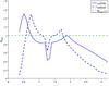 |
Fig. 8 Distribution of MFR twist turns along the z-axis for group 2 shown in Table 1. |
| In the text | |
|
Fig. 9 Evolution snapshots of cases refTDb (top row a) and intkink (bottom row b). The colored curves represent the magnetic field lines outside (blue and orange) and inside (green) the MFR. Translucent isosurfaces indicate the current structures of the MFR. |
| In the text | |
|
Fig. 10 Rotational movement in case refTDb. Panel a: current distributions on two cuts of MFR at t = 5.4, and the current isosurfaces give the geometry shape of MFRs. Panel b: velocity distribution on two cuts; the three green arrows indicate the direction of rotation. The curves show the magnetic field lines passing through discrete points on the z-axis. |
| In the text | |
|
Fig. 11 Disturbances in By as function of time at discrete points on the z-axis for case refTDb (panel a) and case intkink (panel b). The labels on curves are the z-axis coordinate of the sampled points. Sample points below/above the MFR are colored blue/purple. |
| In the text | |
|
Fig. 12 Panel a: colored magnetic field lines whose start points are on the left (green) and right (purple) foot points of MFR at t = 5.4. The red arch represents the initial magnetic axis. Panel b: trajectory of crossing points between the panel y = 0 and magnetic field lines. |
| In the text | |
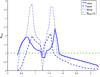 |
Fig. 13 Distribution of MFR twist turns along the z-axis for group 3 in Table 1. |
| In the text | |
|
Fig. 14 Panels a, b: evolution snapshots of MFR for case mixa shown by current isosurfaces from different viewpoints at time t = 2 and 9.6. Panel c: current distribution snapshot on chosen cuts at same time as panel b. Panel d: flux function of poloidal field At on the cut y = 0, and magnetic field lines (blue) rotating around different magnetic axes (red). |
| In the text | |
|
Fig. 15 Panels a, b and c: same as Fig. 14, but for case mixb at t = 3.6 and 15. Panel d: magnetic field lines around the footpoints of MFR (blue) and along the CS (orange). |
| In the text | |
|
Fig. 16 Evolution snapshots of ∫ | j | dz for case mixb (a) and ltirep (b), in which the S-shaped sigmoidal structures form and surround the original MFRs. Panels c and d: evolution snapshots of ∫ | j | dz for cases intkink and infkink to show more possible geometrical features of MFRs. |
| In the text | |
Current usage metrics show cumulative count of Article Views (full-text article views including HTML views, PDF and ePub downloads, according to the available data) and Abstracts Views on Vision4Press platform.
Data correspond to usage on the plateform after 2015. The current usage metrics is available 48-96 hours after online publication and is updated daily on week days.
Initial download of the metrics may take a while.