| Issue |
A&A
Volume 608, December 2017
|
|
|---|---|---|
| Article Number | A140 | |
| Number of page(s) | 13 | |
| Section | Galactic structure, stellar clusters and populations | |
| DOI | https://doi.org/10.1051/0004-6361/201731462 | |
| Published online | 15 December 2017 | |
Proper motions in the VVV Survey: Results for more than 15 million stars across NGC 6544⋆
1 Millennium Institute of Astrophysics, Av. Vicuña Mackenna 4860, 782-0436 Macul, Santiago, Chile
e-mail: This email address is being protected from spambots. You need JavaScript enabled to view it.
2 Instituto de Astrofísica, Pontificia Universidad Católica de Chile, Av. Vicuña Mackenna 4860, 782-0436 Macul, Santiago, Chile
3 Departamento de Ciencias Físicas, Universidad Andrés Bello, Campus La Casona, Fernández Concha 700, 1058 Santiago, Chile
4 Vatican Observatory, 00120 Vatican City State, Italy
5 Millennium Nucleus “Protoplanetary Disks”, 1058 Santiago, Chile
6 Departamento de Ingeniería Eléctrica, Universidad de Chile, Av. Tupper 2007, 1058 Santiago, Chile
7 Universidad de Atacama, Departamento de Física, 485 Copayapu, Copiapó, Chile
Received: 28 June 2017
Accepted: 1 September 2017
Abstract
Context. In the last six years, the VISTA Variable in the Vía Láctea (VVV) survey mapped 562 sq. deg. across the bulge and southern disk of the Galaxy. However, a detailed study of these regions, which includes ~36 globular clusters (GCs) and thousands of open clusters is by no means an easy challenge. High differential reddening and severe crowding along the line of sight makes highly hamper to reliably distinguish stars belonging to different populations and/or systems.
Aims. The aim of this study is to separate stars that likely belong to the Galactic GC NGC 6544 from its surrounding field by means of proper motion (PM) techniques.
Methods. This work was based upon a new astrometric reduction method optimized for images of the VVV survey.
Results. PSF-fitting photometry over the six years baseline of the survey allowed us to obtain a mean precision of ~0.51 mas yr-1, in each PM coordinate, for stars with Ks< 15 mag. In the area studied here, cluster stars separate very well from field stars, down to the main sequence turnoff and below, allowing us to derive for the first time the absolute PM of NGC 6544. Isochrone fitting on the clean and differential reddening corrected cluster color magnitude diagram yields an age of ~11−13 Gyr, and metallicity [Fe/H] =−1.5 dex, in agreement with previous studies restricted to the cluster core. We were able to derive the cluster orbit assuming an axisymmetric model of the Galaxy and conclude that NGC 6544 is likely a halo GC. We have not detected tidal tail signatures associated to the cluster, but a remarkable elongation in the galactic center direction has been found. The precision achieved in the PM determination also allows us to separate bulge stars from foreground disk stars, enabling the kinematical selection of bona fide bulge stars across the whole survey area.
Conclusions. Kinematical techniques are a fundamental step toward disentangling different stellar populations that overlap in a studied field. Our results show that VVV data is perfectly suitable for this kind of analysis.
Key words: Galaxy: bulge / globular clusters: individual: NGC 6544 / Galaxy: kinematics and dynamics
Based on observations taken with ESO telescopes at Paranal Observatory under programme IDs 179.B-2002.
© ESO, 2017
1. Introduction
VISTA Variables in the Vía Láctea (VVV) is a public ESO near-infrared (NIR) survey aimed to obtain the most accurate 3D map of the Milky Way (MW) bulge and inner disk, using variable stars (Minniti et al. 2010).
During its six years of operation, the VVV survey observed approximately 250 deg2 across the inner disk (294.7° ≤ l ≤ 350.0°; −2.25° ≤ b ≤ + 2.25°) and 315 deg2 in the bulge of the MW (−10° ≤ l ≤ + 10.4°; −10.3° ≤ b ≤ + 5.1°). Thanks to the use of multicolor NIR bands (ZYJHKs), VVV data can penetrate gas and dust in the plane, exploring yet unknown regions of the MW. At the same time, the ~80 epochs in Ks provide the opportunity to search for signs of variability in about a billion sources (Saito et al. 2012) in the region where most of the stars in the MW are confined.
The study of the inner regions of the MW is difficult for several reasons. The high and spatially variable dust extinction mentioned above can be minimized using NIR bands. Crowding is also an issue that requires relatively good seeing (~1 arcsec for VVV data) and a small pixel scale (0.34 arcsec in VIRCAM) and in our case becomes critical only for stars in the lower main sequence. Another problem, however, still affects the interpretation of the photometry: the presence of more than one population along the line of sight. A large number of foreground disk stars, mostly in the main sequence but also in the red giant and core helium burning phases, are seen along any line of sight toward the bulge. In addition, the study of star clusters toward the bulge is complicated by the presence of both disk and bulge stars, not easy to tell apart from the color magnitude diagram (CMD) alone.
An efficient way to disentangle different populations in any stellar field is by means of proper motion (PM) analysis, a well known technique that helps to isolate kinematically the contribution of the different stellar components across the area under study. PM measurements are one of the most promising methods to study the Galactic bulge. As a matter of fact, unlike external galaxies the stars in the MW bulge are close enough that is possible to resolve them and study the stellar populations and stellar kinematics in detail. However, our location inside the disk has limited the optical observations mainly to carefully selected low-extinction windows toward the center, or to relatively shallow (optical) images in regions with poorer visibility conditions. The first PM investigation of the Galactic bulge was made by Spaenhauer et al. (1992) and since then, several additional studies have been followed (Mendez et al. 1996; Sumi et al. 2004; Vieira et al. 2007, among others). Many studies have exploited the exquisite precision astrometry provided by space-based images (Kuijken & Rich 2002; Clarkson et al. 2008; Soto et al. 2014), however limiting their analysis to tiny regions in the sky.
The current instrumentation has improved to the point that today is possible to apply successfully PM techniques to data taken from ground-based telescopes with relatively short time coverages. A decade ago, Anderson et al. (2006) adapted the methods developed for high-precision astrometry and photometry with the Hubble Space Telescope (HST) to the case of wide-field ground-based images and described in detail the steps that are necessary to achieve good astrometry with wide-field detectors. To test the method, Anderson et al. (2006) computed PMs for the two closest Galactic globular clusters (GCs), showing that ground-based observations with a time span of a few years allowed a successful separation of cluster members from Galactic field stars. In the following years, the same technique was applied to more distant GCs (Bellini et al. 2009; Zloczewski et al. 2011; Sariya et al. 2012, 2017; Sariya & Yadav 2015) and open clusters (Yadav et al. 2008, 2013; Montalto et al. 2009; Bellini et al. 2010). Recently, Libralato et al. (2015) followed the same prescription to compute PMs in the field of the GCs M 22 using four years of VVV data.
The large coverage in space and time of the VVV survey opens the opportunity of using PM techniques to study an area across the sky that includes the whole Galactic bulge, part of the southern disk, ~36 globular clusters and thousands of open clusters. The VVV observations are now complete, providing a time baseline of more than five years for PM studies in addition to stellar variability. To this aim, we have developed an automated code to derive PMs in VVV data, following the approach described in Anderson et al. (2006) and Bellini et al. (2014). As a test of its precision, we applied our method to the field including the Galactic GC NGC 6544.
NGC 6544 (see Fig. 1) is a relatively metal poor (Fe/H = −1.4 dex; Harris et al. 1996) GC located at a projected distance of ~6 kpc from the Galactic center, specifically at (l,b) = (5.84,−2.2). Its position in the sky against the Galactic bulge and disk implies that a large contribution of field stars contaminate its CMD, making the identification of cluster members from photometry alone highly uncertain. This explains why this cluster has been the target of only a few photometric and spectral studies. Thanks to the cluster proximity (d = 2.5 kpc; Cohen et al. 2014), cluster giants are bright and easy to separate from field stars, in the CMD. Below the main sequence turnoff, however, the only reliable way to disentangle the different populations is to use PMs. To date, the only attempt at deriving PMs was carried out by Cohen et al. (2014). They computed relative PMs between cluster and bulge stars, in order to select bona-fide cluster members in the (40′′ × 40′′) area covered by the PC/WFPC2 camera on board HST. Their purpose was to obtain accurate physical parameters of the cluster inner region rather than to derive precise PMs over a wide area. Cohen et al. (2014) suggest that the cluster is possibly losing stars due to the gravitational interaction with the MW. This makes a wide area PM study particularly interesting, in order to look for possible cluster extended tidal tails.
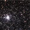 |
Fig. 1 Color image of chip #15, in pawprint #2 of VVV field b309. The field of view of this image is 12′ × 12′; north Galactic pole is up, positive galactic longitudes are left. |
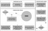 |
Fig. 2 Flow chart illustrating the three main steps adopted to computed PMs and explained in detail in the text. |
2. Proper motions
Relative PM studies are often based on the comparison of two sets of images taken in two observing runs, separated by a few years. The data from each observing runs are grouped and considered as a single epoch, and the PM is derived from the position difference of each star between the two epochs. In the present case, the data from the VVV survey extend almost continuously across a time span of approximately six years, favoring the approach described by Bellini et al. (2014). The latter considers each image as a single epoch, and fits the PM of each star, in each of the x- and y-axis, as the derivative of the linear relation between the star pixel coordinate and the time. In this section we describe how this method was optimized to derive PMs for stars in the VVV images, applied to a field including the GC NGC 6544. Figure 2 summarizes the steps adopted to find the initial star list, create the master (reference) catalog, and finally compute PMs. The details of each of these steps are described in the three subsections below.
2.1. PSF photometry and the initial master list
The data obtained for the VVV survey comes from the VISTA/VIRCAM instrument, an array of 4 × 4 Raytheon VIRGO detectors of 2048 × 2048 pixels each, with an average spatial resolution of ~0.̋339 pixel-1 (Dalton et al. 2006; Emerson & Sutherland 2010). Each individual science image, called pawprint, is composed of two exposures dithered by 40 pixels in order to remove detector artifacts. At each sky pointing, six dithered pawprints are acquired in such a way that they can be combined in a single mosaic, called a tile, filling the large gaps between the 16 VIRCAM detectors. All pawprints are processed through the standard CASU pipeline for bias subtraction, dark correction and flat-fielding (Emerson et al. 2004; Irwin et al. 2004). For the present work, PSF-fitting photometry was performed separately on each given detector of a given pawprint, and the PMs were derived from the comparison of all the epochs of that specific detector. Other nearby detectors were ignored here, even if, because of dithering, in different pawprints they cover part of the same sky area. For example, we initially started the analysis on the detector covering most of the cluster area. That was chip #15 (out of 16) of pawprint #2 (out of 6) of each observation available for the VVV field b309. A Ks image of this chip is shown in Fig. 1. All the available epochs for chip #15 of pawprint #2 were downloaded from the ESO archive. In each of the ZYJHKs filters, we retrieved 3, 4, 2, 2, 327 epochs, respectively, each covering ~12 × 12 square arcmin. The PM analysis is based on the Ks data alone, which were acquired between April 2010 and September 2015. PSF fitting photometry on each image was carried out using the DAOPHOTII/ALLSTAR package (Stetson 1987), with a Moffat (1969) PSF model constructed using the brightest, isolated and non saturated stars in each image. Initial stellar positions and fluxes were measured independently on each image, with a relatively high detection threshold (30σ) and a first run of ALLSTAR on all of them. This ensured that only stars with good photometric quality and accurate positions were kept for the coordinate trasformation step. We then selected one of the images with best seeing to be used as reference coordinate system (refframe) and run the DAOMATCH/DAOMASTER (Stetson 1994) codes to determine accurate frame-to-refframe coordinate transformations for each image. A stacked mean image was then created using the MONTAGE routine of the same package. The latter has high signal-to-noise (S/N) ratio, it is free of cosmic rays, and it has a field of view (FoV) slightly larger than any single epoch. We will refer to this stacked mean image as the master-image. The star finding (FIND) routine of DAOPHOT was run on the master-image, now with a smaller detection threshold (3σ), together with the aperture photometry task (PHOT). The resulting master-list, after an inverse coordinate transformation, has been used as input for the ALLSTAR PSF-fitting photometry routine on each individual image, allowing the code to refine the position of the centroids (ALLSTAR parameter RE = 1). A side advantage of this approach is that a unique ID number identifies a given star in all the epochs. The instrumental magnitudes were calibrated to the VISTA photometric system using ~15 000 stars in common with the public CASU catalogs derived for the same epochs, by means of a simple magnitude shift. The final photometric catalog was obtained by averaging the magnitudes of the individual epochs. It contains 140 000 stars, from the upper red giant branch (RGB) down to approximately three magnitudes below the main sequence turnoff, as shown in Fig. 3. The cluster sequences, on the blue side of the CMD in this figure, are contaminated by a well populated bulge RGB (parallel to the cluster RGB, but to the red) and main sequence, both with a large spread in magnitude and color due to differential reddening (and to less extent due to distance), and by the main sequence of the foreground disk, bluer and brighter than the cluster turnoff. We note that the cluster’s evolutionary sequences in the CMD are less broadened than the bulge ones, suggesting that most of the reddening is behind the cluster. The actualevidence from dust behind the cluster is the “great dark lane” that runs across low latitudes toward the bulge discovered by the VVV survey (Minniti et al. 2014). The cluster is located in the same direction of this great dark lane shown in the left panel of Fig. 2 in Minniti et al. (2014).
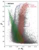 |
Fig. 3 CMD for all the stars detected in the field shown in Fig. 1. The hand drawn blue line shows the approximate location of the cluster sequences, while the red and green areas show the bulge RGB and disk MS, respectively. |
2.2. The master catalog
The previous steps yields a photometric catalog for each individual epoch. In order to compare the position of each star in all these epochs, we need to ensure that the pixel scale is uniform across the field of view. That is because a given star may fall on slightly different positions within the field, on different epochs. To this end, the geometric distortion correction specifically derived for the VIRCAM camera in Libralato et al. (2015) has been applied to each catalog. This correction provides distortion-free coordinates with residuals of the order of 0.023 pixels.
We then need to define a master catalog, to use as zero point reference in the computation of the displacement of each star, in each epoch. This was done by selecting ~10 000 well measured stars in common among all the epochs, and use them to derive six-parameter linear transformations between each distortion-corrected catalog and the epoch (refframe) previously used as reference for the coordinate transformations described in Sect. 2.1. These transformations were then applied to each catalog, in order to obtain, for each star, Nepochs positions that it would have, if it had no PM, in the refframe system. For each star, these Nepochs positions were then averaged to derive a single (Xref,Yref) pair, that will be the reference point for the calculation of all the ΔX = Xi−Xref and ΔY = Yi−Yref, with i = 1,Nepochs. The catalog with the reference positions for all the stars is our (initial) master catalog. The latter is iteratively refined, by going back to the determination of the six-parameter linear transformations, this time with respect to the master catalog instead of the refframe one. Convergence was typically achieved in less than five iterations.
It is worth emphasizing that the advantage of creating a reference master catalog, instead of using a single epoch, is that the reference catalog contains more stars than any single epoch catalogs. At this stage the coordinate transformations used to create the master catalog are global for the whole detector, rather than local as they will be in the actual PM calculation (see below). This does not introduce more scatter because the positions in the master catalog define the zero point of the coordinate displacement of each star. Because the PM will be the slope of the ΔX (or ΔY) vs time relation, if the zero points are slightly different for stars located in different regions of the field, this does not affect the PM calculation.
2.3. Deriving proper motions
In order to derive the PMs, we will now transform the coordinate of every star, in each single epoch, to the coordinate system of the master catalog created above. Then, the displacement of each star in each epoch with respect to the master catalog will be calculated, relative to the displacement of a sample of nearby stars selected as reference population. In other words, we will calculate how much starN has moved, compared to how much its nearby stars have moved. This relative displacement, both in X and Y, is then plotted against time, and fitted with a linear relation whose slope (relative movement per unit time) is by definition the PM of starN along the X and Y-axis.
An example of the PM of a star with magnitude Ks = 12.40 mag is shown in the upper panel of Fig. 4. A 3σ clipping has been applied before the least square fit. The error on the derived slope is, by definition, the statistical error (SE) on the PM in each axis. The combined statistical error (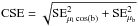 ), as a function of Ks magnitude is shown in the lower panel of Fig. 4 for all the stars. The distribution of the PM CSE at each given magnitude is obviously skewed, with a long tail toward large PM errors. Two lines, representing the median PM CSE for the unclipped stars and a 3σ clipping of the distribution are included for comparison. The mean CSE in bins of 0.5 mag is also indicated. The inset shows the histogram of the PM CSE for stars with 11.5 <Ks< 15 mag before and after the 3σ clipping. The mean CSE within this magnitude range is 0.50 mas yr-1.
The astrometric reference stars selected for the present work were bulge RGB stars. In previous studies (e.g., Bellini et al. 2014; Libralato et al. 2015) it has been common to select cluster stars, because they have a smaller internal velocity dispersion, that is, they move coherently. Bulge stars on the other hand, have a larger velocity dispersion, therefore one needs a larger sample of them in order to average out the different individual motions. They have been preferred in this work because our ultimate goal is to design a method that can be applied to the whole VVV bulge area, even far away from star clusters.
Well measured, non saturated bulge RGB stars were initially selected based on their location in the CMD (see Fig. 3) and their small photometric error. After the first iteration in the calculation of PMs, this initial selection will be refined adding their PMs as a selection criterion. Iterations are repeated until the number of selected reference stars converges.
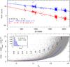 |
Fig. 4 Top: example of PM determination by means of the least square fitting for one of the cluster stars (#98166), with magnitude Ks = 12.4 mag. Each point is the star position in different epochs after been locally-transformed to the reference system of the master catalog. Bottom: CSE in the PM, computed as the error on the slope in the linear fit shown above, as a function of Ks magnitude. The thin red line marks a 3σ clipping on the error distribution; the thick blue line is the median error. Numbers list mean errors in bins of 0.5 mag. The figure inset shows the histogram of errors for 11.5 <Ks< 15 mag before (gray) and after (blue) the 3σ clipping. |
Following (Anderson et al. 2006), the transformations used in the last step of the PM calculation are local, that is, restricted to a small region of the chip close to each starN. This is more time consuming, but it ensures that residual astrometric distortions across the field of view of each chip do not have an impact on our results. Specifically, in this work the displacement of each star, in each epoch, was calculated with respect to a sample of the closest reference stars provided they are between 10 and 50 in number, and are located within a distance of 300 pixels from the center of starN. Stars with less than 10 reference stars were not analyzed. These nearby reference stars were used to derive a linear local transformation between each epoch and the reference catalog, valid only for starN. The final PM in pixels yr-1 was then converted to mas yr-1 by means of the VIRCAM pixel scale (0.̋339 pixel-1).
3. Kinematical decontamination of the cluster’s CMD and error budget
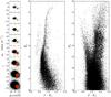 |
Fig. 5 Left: vector point diagrams for all the stars detected in the field, divided in eight one-magnitude bins according to the CMDs on the right. The green circle shows the adopted membership criterion used to selected cluster members in each magnitude interval. We adopted a radius of 4 mas on the brightest bin and allowed a bigger selection region for poorer measured stars (7.5 at the bottom). Middle: clean CMD for the stars assumed to be cluster members (red points inside the green circle in the VPD). Right: CMD for the field counterpart after excluding likely cluster stars. |
The main result of our PM analysis is illustrated in Fig. 5. On the left we show the Vector Point Diagram (VPD) of all the stars plotted in Fig. 3 in steps of magnitude, increasing toward the bottom. We can clearly separate (at least) two kinematically distinct populations, a warmer one roughly centered at the zero of the VPD, and another one with lower dispersion, centered at (μlcos(b),μb) ~ (−10.6,−6.6) mas yr-1. By construction, because we choose bulge stars as reference, the cloud centered at (0, 0) mas yr-1 is made of bulge stars, while the tighter clump is made up of cluster stars.
Bona fide cluster stars were selected as those having PMs within the small green circle, centered in the tight clump. The calculation of the center of this circle is explained in Sect. 5. The radius was arbitrarily chosen to vary smoothly between 4 mas yr-1 for the brightest stars and 7.5 mas yr-1 for the faintest ones. Cluster stars selected in this way, and marked in red in the left panels, are plotted in the middle panel of Fig. 5. All the other stars, marked in black in the VPD, are mostly field stars and are shown in the right panel of the same figure. As expected, cluster stars lie along relatively narrow sequences in the CMD, showing a blue horizontal branch and a well defined main sequence turnoff at Ks ~ 15.5 mag. Field stars, on the other hand, show the usual bulge + disk CMD, with a prominent bulge RGB, a red clump at (J−Ks, Ks) ~ (1.5, 13) mag, both of them widely spread in color due to differential extinction, and the disk main sequence on the blue side (see Fig. 3).
The PM distribution of cluster stars and the SEs obtained in the previous section allow us to estimate the total error of our method. Indeed, the spread of cluster stars in the VPD is the convolution of the real PM dispersion due to the orbital motion of cluster stars and the total (statistical + systematic) PM error. The observed dispersion of cluster stars in the VPD was calculated by selecting non-saturated stars with Ks< 15 mag, and PM CSE smaller than 3σ, resulting in a dispersion of 0.77 mas yr-1. The central velocity dispersion of NGC 6544 is not included in the Harris catalog, but according to the spectroscopic analysis by Gran et al. (in prep.) seven confirmed NGC 6544 member stars have a radial velocity dispersion σ ~ 6 km s-1. The analyzed stars are located at a mean distance of  from the cluster center, thus imposing a lower limit for the central velocity dispersion of the cluster. Adopting a cluster distance of 2.5 kpc (Cohen et al. 2014) this corresponds to an intrinsic PM dispersion of 0.51 mas yr-1. Subtracting in quadrature this value from the observed dispersion in the VPD, we derive a total error of 0.57 mas yr-1, in each component, valid for cluster stars with Ks< 15 mag. As mentioned above, this is the combination of the SE plus the contribution of several possible sources of systematics, such as geometrical-distortion residuals, image motion, differential chromatic refraction, S/N bias, local-transformation bias, among others (see e.g., Anderson et al. 2006; Bellini et al. 2014; Libralato et al. 2015, and references therein). The CSE was derived in Sect. 2.3 from the slope of the relations shown in Fig. 4 for all the stars, resulting in 0.50 mas yr-1. The total error estimated above, however was calculated for cluster stars, which are, on average, more crowded than field stars, and therefore have slightly larger SEs. Indeed, if we repeat the calculation in Fig. 4 for cluster members only, we get a mean CSE of 0.62 mas yr-1. By subtracting in quadrature the SE (~
 ) from the total errors estimated above (0.57 mas yr-1) we conclude that the contribution of the systematics to the error budget is 0.37 mas yr-1 along each galactic coordinate. The total error for field stars in each coordinate can now be estimated by adding in quadrature this systematic (0.37 mas yr-1) to the SE measured in Sect. 2.3 for disk and bulge stars separately (0.40 and 0.32 mas yr-1), which yields 0.54 and 0.50 mas yr-1, respectively.
4. The disk-bulge relative proper motion
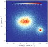 |
Fig. 6 Hess diagram of the VPD for all the stars with PM CSE lower than 10 mas yr-1. Stars belonging to NGC 6544 cluster in the lower right corner, while field stars are the cloud around zero. This cloud is significantly elongated along the longitude axis, because of the presence of two populations, disk and bulge, with the disk having a significant rotation. |
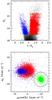 |
Fig. 7 Top: CMD showing our selection of RGB bulge stars (red) and main sequence disk stars (blue) after excluding likely cluster members. Bottom: VPD showing the relative PM displacement between the selected stars from the CMD. NGC 6544 stars have been included in green for comparison. |
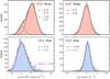 |
Fig. 8 PM distribution of bulge and disk stars selected as shown in Fig. 7. Left panels: μlcos(b) distributions. The disk distribution is well fitted with a single Gaussian (black solid line) if the positive tail is excluded. The otherwise better skewed Gaussian fit is shown with a dashed magenta line. The bulge distribution is fitted with two Gaussians, with the centroid of the leftmost one fixed to the value found for the disk. Right panels: μb distributions of bulge and disk are symmetric, allowing a clean fit with one Gaussian. In all panels, centroid and dispersion of the fitted profiles are quoted. |
Figure 6 shows the VPD for all the stars with CSE lower than 10 mas yr-1 (see Fig. 4) color coded according to the density of stars. The PM distribution for field stars is highly elongated along the longitude axis, suggesting either a large rotation or the presence of two populations (or both). In fact, from the Galactic position of the cluster, and from the total CMD, one would expect the presence of disk stars in front of the cluster and both disk and bulge stars behind it. In order to trace the position of disk and bulge stars in the VPD, in Fig. 7 (top panel) we select a sample of bona fide disk stars, in the upper MS, and a sample of bona fide bulge RGB stars. These two populations partially overlap in the VPD (bottom panel), although disk stars are flatter in this plane, due to their smaller velocity dispersion and larger rotation. To compute the centroids and dispersion of both components, we use the PM histograms shown in Fig. 8 to plot the bulge and disk stars selected in Fig. 7. As can be seen, along the Galactic longitude axis the PM distribution of the bulge (upper left panel) shows a secondary bump located at μlcos(b) ~ 5.0 mas yr-1, which coincides with the peak of the disk distribution in the same direction (lower left panel). This feature is produced by disk stars in the RGB evolutionary sequence. Taking this into account the procedure was the following: we started analyzing the disk component shown in the lower left panel of Fig. 8 where the best fit was found to be a skewed Gaussian, shown with a dashed magenta line. To overcome this asymmetry, the distribution was truncated at μlcos(b) = 2.0 mas yr-1 which allowed a single symmetric Gaussian centered at μlcos(b) = 4.78 mas yr-1 to be fitted. Fixing the disk centroid value to perform a double Gaussian fitting of the bulge component along the same axis, the centroid of this component was found to be at μlcos(b) ~ −0.4 mas yr-1. The dotted lines in the upper left panel of Fig. 8 are the two fitted Gaussians whose sum is the solid line. Along the latitudinal axis, both components show a symmetric distribution, thus allowing a clean fit with one Gaussian each. Notice that the exclusion of disk stars when fitting the bulge component along the longitude axis moved the latter slightly off from the (0,0) position where reference stars are centered by construction. The described procedure resulted in an offset of the disk with respect to the bulge RGB centroid, by a Δμlcos(b) = 5.2 ± 0.04 mas yr-1 and Δμb = −0.63 ± 0.04 mas yr-1, somewhat higher when compared with the relative velocities found in previous studies by Clarkson et al. (2008) and Vásquez et al. (2013). The bulge RGB stars, have an observed dispersion of (σl,σb) = (2.33 ± 0.02,2.02 ± 0.02) mas yr-1. Deconvolving these values from the total PM errors estimated in Sect. 3 (errl = 0.50, errb = 0.50) mas yr-1 we obtain (σl,σb) = (2.28 ± 0.02,1.96 ± 0.02) mas yr-1, slightly smaller than the values obtained by Soto et al. (2014) and Kuijken & Rich (2002) but in very good agreement with Zoccali et al. (2001). The mild PM anisotropy found σl/σb = 1.16 is in perfect agreement with Zhao (1996) and is explained as the effect of the bulge mean rotation.
5. NGC 6544 space velocity
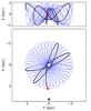 |
Fig. 9 Computed orbit for NGC 6544 using an axisymmetric model. The actual location of the cluster is indicated by a red dot while the position of the Sun by a black cross. Blue and black paths show the orbit of the cluster 3 Gyr back and 0.25 Gyr ahead in time, respectively. |
In order to compute the space motion of NGC 6544 we first determine the relative PM of the cluster with respect to the bulge, as the offset between their centroids in the VPD. To this end, only clusters stars with Ks< 15 mag and PM CSE below the 3σ limit (see bottom panel of Fig. 4) were selected, to calculate their mean PMs in both axis. The centroid of NGC 6544 turned out to be at (μlcos(b),μb) = (−10.57 ± 0.03,−6.63 ± 0.03) mas yr-1. Subtracting the latter from the value of the bulge centroid computed in the previous section we obtain a relative motion of the cluster stars with respect to the bulge Δμlcos(b) = −10.17 ± 0.04 mas yr-1 and Δμb = −6.62 ± 0.04 mas yr-1. To determine absolute PMs for the cluster, we have cross-correlated the cluster catalog with the UCAC5 catalog recently published by Zacharias et al. (2017) obtaining 330 stars in common. From their comparison, we computed a mean relative shift of −6.34 ± 0.39 and −1.09 ± 0.39 mas yr-1 along galactic longitude and latitude, respectively. The derived absolute PM for NGC 6544 resulted in (μlcos(b),μb) = (−16.91 ± 0.39,−7.72 ± 0.39) mas yr-1. In order to trace the orbit of the cluster, given the current absolute PMs, we have used the program galpy develped by Bovy (2015) adopting for NGC 6544 a heliocentric radial velocity of Vr = −27.3 km s-1 from Harris et al. (1996) and a distance d = 2.5 kpc from Cohen et al. (2014). Moreover, we have asumed a Solar motion with respect to the Local Standard of Rest of (U⊙,V⊙,W⊙) = (11.1,12.24,7.25) km s-1 from Schönrich et al. (2010), a rotational velocity of the LSR of 220 km s-1 and a distance of the Sun to the Galactic center of 8.2 kpc (Bland-Hawthorn & Gerhard 2016). The calculation requires the assumption of a potential, that in our case includes three components, a spherical component (bulge) with a power-law density distribution and an exponential cut-off, a Miyamoto-Nagai disk, and a Navarro Frenk and White halo potential (Navarro et al. 1997). The orbit has been sampled 10 000 000 times using a Runge-Kutta 6th integrator, in a time interval corresponding to −3 Gyr to + 250 Myr. Figure 9 shows the orbit of NGC 6544 projected in the XY and RZ planes. In our integration, the cluster reaches to be closer than ~0.5 kpc to the galactic center. As discussed by Minniti (1995) and Bica et al. (2016), Galactic GCs can be divided in bulge, disk and halo GCs according to their metallicity, relative position and kinematics. Taking into account its relatively low metallicity and based on the integration of this simple potential, we find that NGC 6544 is more consistent with the halo population than with the bulge or disk components. It should be noted, however, that the bulge potential assumed here is axisymmetric, which is certainly an oversimplification.
6. Membership probabilities
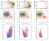 |
Fig. 10 Upper row: membership probability as a function of magnitude for the bulge, disk and cluster, color coded by point density. The blue and red dashed lines depict the p = 0.66 and p = 0.90 levels used to select likely members of the respective components of the mixture. Middle row: VPD of the whole sample is displayed identically in each panel, color coded by density. The blue and red points stand for subsamples of bulge, disk, and cluster stars selected as those with membership probabilities to the respective component larger than p = 0.66 and p = 0.90 (and with error in their probabilities smaller than 0.35). Lower row: CMD for the most probable members of the bulge, disk and cluster, color coded as above. |
In order to calculate the likelihood of each star to belong to the disk, bulge, or GC we consider a probabilistic approach based on the Bayesian partial membership (BPM) model for continuous data (Heller et al. 2008; Gruhl & Erosheva 2014; Blei & Laffertyet 2007). Contrary to standard mixture models, partial membership models do not restrict data samples to belong to only one of the constituent distributions, but allows data points to have fractional membership to multiple components. In the BPM each data point is modeled as arising from a geometric average of the constituent distributions weighed by a membership probability vector πi ∈ [0,1] K such that  (Heller et al. 2008). In other words, each data point has an associated membership probability vector πi which relates it to the components of the mixture. This approach allows modeling data in scenarios with high overlap between the generating distributions, for example, the samples coming from the disk and the bulge. In the present case we have a three-component mixture model, that is, K = 3. We set the components of each population as a multivariate normal distribution MvN(μk,Σk), where a full covariance and a single variance matrix (Σ = Iσ2) are adopted in the case of disk/bulge and cluster, respectively. In order to define values for the mean vector and dispersion of each MvN distribution in the VPD, we consider only bright stars (Ks ≤ 15 mag) with PM CSE ≤3 mas yr-1. The centroids of the bulge, disk and cluster are known and kept fixed at (μxb,μyb) = (−0.40,0) mas yr-1, (μxd,μyd) = (4.78,−0.62) mas yr-1 and (μxc,μyc) = (−10.57,−6.63) mas yr-1, respectively. In the same vein, initial values for the scale parameter, that is, the diagonal of the covariance matrix, were set to
  ,
,  and
and  , corresponding to the intrinsic PM dispersion (observed dispersion deconvolved by the total PM errors) of each population. The associated errors of each individual PM measurement and weakly informative priors were also included in the covariance matrices of the components. A detailed description of the hierarchical model and the specification of the priors can be found in Appendix A. In order to compute membership distributions, covariance components and their respective priors we use an optimization approach based on automatic differentiation variational inference (ADVI; Jordan et al. 1999; Kucukelbir et al. 2017). We run the ADVI procedure for approximately 1000 iterations and after convergence, new estimations of mean values and standard deviations for the model parameters were drawn from the variational distribution. The described procedure was run on a sample containing 280 000 stars located in the inner 12′ from the cluster center and with PMs errors lower than 10 mas yr-1. The average concentration of the bulge, disk and cluster found after convergence are 0.847, 0.145, and 0.0074, respectively.
Figure 10 summarizes the main results of this analysis. The top panels show the average membership probabilities as a function of Ks magnitudes in the PM space, for each of the three elements of the mixture. The upper right panel shows that likely cluster members, that is, stars with more than 90% membership probability to belong to NGC 6544 separate clearly from field stars down to at least Ks ~ 16 mag. For fainter magnitudes the PM errors become larger and therefore many stars have a lower probability to belong either to the cluster or to the field, that is, the two distributions merge. This effect is even clearer in the VPDs shown in the middle panels. There we highlight the stars with probabilities higher that 66% and 90% of belonging to the cluster (right), disk (middle) or bulge (left) populations. In particular, stars with 90% probability of being cluster members set aside from field stars, while for probabilities lower than ~70% the cluster blob merges with the bulge+disk one and the contamination from the field steadily grows. The bottom panels of Fig. 10 show the CMD for bulge, disk and cluster stars obtained using the same color code as the middle panels. As can be seen, stars with a 90% probability of being cluster members can be found even ~2 mag below the main sequence turnoff. This kind of quantitative assessment of the probability membership of each star will be particularly relevant in the context of future spectroscopic follow-ups of cluster (or bulge and/or disk) stars.
7. Metallicity, interstellar reddening and age
A major benefit of the membership probability analysis is that we can now separate the cluster population from the field stars and produce a CMD with the most likely cluster members. However, differential reddening can still produce a significant width on the evolutionary sequences of the cleaned CMD. To correct for this effect, a relatively extended field centered in NGC 6544 was divided in 64, 2′ × 2′ square subfields. One of them with well defined and populated sequences was selected to be the reference subfield. A fiducial line was extracted from it and used to apply the technique described in Piotto et al. (1999). Namely, the CMD of each subfield is shifted along the reddening vector to match the fiducial line of the reference CMD. In this manner we obtained the CMD corrected for differential reddening of each single subfield.
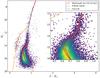 |
Fig. 11 CMD including only those stars with Pc(i) greater than 70% of being cluster members. The blue solid lines represent the ridge line obtained using VVV data. We adopted a distance modulus of DM0 = 11.96 from Cohen et al. (2014) to match the isochrones from Dartmouth (red) and PGPUC (yellow) databases. The inset shows that, at the level of the SGB-MS, the best fit of the isochrones with the fiducial line is obtained for an age between 11 and 13 Gyr. |
Selecting only stars with membership probability higher than 70% from the reddening corrected CMD, the main evolutionary sequences of NGC 6544 can be easily traced and can be used to derive reliable cluster parameters as shown in Fig. 11. Most of the bright stars in this CMD (Ks< 12.0 mag) are saturated in the VVV catalogues. Accordingly, they were included here from the photometry by Valenti et al. (2010), transformed from the 2MASS JHKs system to the VISTA JHKs system using the most up to date color transformations from Gonzalez-Fernandez et al. (in prep.). To determine the metallicity and reddening of the cluster, the fiducial line was used to match at the RGB level a set of isochrones from the Dartmouth stellar evolution database (Dotter et al. 2008), adopting the distance modulus derived by Cohen et al. (2014, DM0 = 11.96 mag). The best coincidence was obtained for values of −1.5 dex and 0.36 mag in metallicity and reddening respectively. We note that across the studied area, the computed reddening varies between 0.34 to 0.66 mag and therefore the value given here applies only to the area selected to constructed the fiducial line of the cluster. We also have included a zero-age horizontal branch isochrone from the PGPUC database (Valcarce et al. 2012) transformed to the filters used in the VVV survey. We have excluded the hydrogen burning locus in the analysis since these isochrones do not include He diffusion along the RGB phase, which in this particular case produces a clear shift to the blue when comparing with isochrones from the Dartmouth database for the same adopted distance and metallicity values. The fit with the horizontal branch population confirms that the adopted distance modulus is correct within the observational errors. In order to estimate the age of NGC 6544, we visually compared the fiducial line with the five isochrones that best match our data, representing ages from 10 to 14 Gyr respectively (see Fig. 11). As the inset of Fig. 11 shows, the fiducial line of the cluster falls down along the sub giant branch and main sequence intersecting the three innermost isochrones, suggesting that the age of NGC 6544 lies between 11−13 Gy.
8. Elongation of NGC 6544
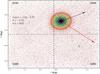 |
Fig. 12 Galactic coordinate map of the area covered by the tiles b295, b296, b309 and b310. Black points depict the position of likely cluster stars with low PM errors. A color map highlights their surface count density, and a set of contour lines is drawn around the center of NGC 6544. The black and red arrows points toward the Galactic center and along the direction of the cluster orbit, respectively. The cluster center, eccentricity of the outermost contour line, and the angle between its major axis and the Galactic equator are quoted. |
Based on the cluster rather flat radial density profile and inverted mass function, Cohen et al. (2014) suggested that it might be more extended than previously thought, loosing stars due to the gravitational interaction with the Galaxy. PMs can be very helpful to trace cluster members well outside the tidal radius, hence we decided to extend our analysis to a region ~3° × 2° wide across the cluster. Specifically, we applied the procedure described in Sect. 2 to tiles b295, b296, b309 and b310, compiling a PM catalog for more than 15 million stars. In order to identify probable cluster members, we have selected stars with PM CSE smaller than 1.5 mas yr-1 (Ks ≲ 15.5 mag) and within a radius of 2 mas yr-1 centered at (−10.57,−6.63) in the VPD. The resulting sample includes 11 217 stars, whose spatial distribution is shown in Fig. 12. The map shown here, at the distance of NGC 6544, corresponds to an area of 129 × 96 pc2. Far from the cluster center, the map shows a rather uniform distribution of stars, evidence that a small contamination from the field is still present inside the “cluster” zone of the VPD. If tidal tails would be present, however, we would expect an enhancement of this density in the direction of the cluster orbit, which is not seen. Obviously, we are considering here only stars with mass slightly smaller than about 0.8 M⊙ (Ks ≲ 15.5 mag). The present data do not allow us to rule out the possibility that, due to dynamical segregation, the stars that were tidally stripped were only the low mass ones.
In Fig. 12 we also show the surface stellar density, obtained via a Gaussian kernel estimation (with a kernel bandwidth set by the custom Scott’s rule). The spatial distribution of cluster stars across the inner ~12 arcmin from the cluster center is clearly elongated. This shape is accentuated by a set of contour lines, which were used to estimate an axial ratio b/a = 0.82. According to the elongation values presented by Chen & Chen (2010) for 116 Galactic GCs, NGC 6544 is among the 30% most elongated clusters. Interestingly, the cluster elongates roughly in the direction pointing toward the Galactic center. The origin of this morphological signature might be related with the gravitational potential of the MW causing a tidal perturbation in the direction of the Galactic center, an encounter with the Galactic plane or by a relatively high rotation of NGC 6554. However, according to Chen & Chen (2010), those GCs close to the bulge and exhibiting obvious flattening tend to have their elongation pointing toward the Galactic center due to tidal effect from the bulge. This is in very good agreement with the results obtained in Sect. 5, where the simulated orbit locates NGC 6544 as close as 0.5 Kpc from the Galactic center.
9. Summary and conclusions
In this paper we described the procedures adopted by our team to compute PMs using VVV data. In particular we have followed the local coordinate transformations approach described by Anderson et al. (2006) and Bellini et al. (2014). In order to validate the method, we have applied it to a region ~3° × 2° wide (4 tiles), toward the MW bulge, including the GC NGC 6544. The six-year time baseline of Ks-band observations provided by the VVV survey allowed us to achieve a typical accuracy in each PM coordinate lower than 0.51 mas yr-1 (statistical + systematics), for Ks< 15 mag gradually increasing up to 10 mas yr-1 at Ks = 18 mag. The PMs allowed us to establish solid membership for cluster stars, which separate very well from field stars in the VPD, and to derive for the first time, the absolute PM of this system, resulting in (μlcos(b),μb) = (−16.91 ± 0.39,−7.72 ± 0.39) mas yr-1.
Based on the computed PMs and spatial distribution, we applied a BPM model to select the most likely cluster members, and produced a decontaminated CMD, essentially free of field stars. Additionally, we correct for differencial reddening, allowing us to better define the evolutionary sequences in the CMD. From the comparison of the clean and differential reddening corrected cluster CMD with isochrones from Dartmouth database, the metallicity and reddening of the cluster were derived, finding values in good agreement with those from literature. Additionally, an age of ~11−13 Gyr was estimated for NGC 6544. Combining PMs and the values for the distance and radial velocity taken from literature, we computed the Galactic orbit of this cluster assuming an axisymmetric model for the MW gravitational potential. Based on this simplified assumption, we concluded that NGC 6544 is likely a GC associated with the halo component of our Galaxy. This is in accordance with its low metallicity (Fe/H ~ −1.5 dex), given that bulge clusters are usually relatively more metal rich (Minniti 1995; Bica et al. 2016).
The PM distribution of both disk and bulge stars were also obtained in this work. The relative PM between the two was found to be (Δμlcos(b),Δμb) = (5.2 ± 0.04,−0.63 ± 0.04) mas yr-1, while the PM dispersion of bulge and disk stars, along each galactic axis was measured to be σμlcos(b) = 2.28 ± 0.02, σμb = 1.96 ± 0.02 and σμlcos(b) = 2.41 ± 0.04, σμb = 1.30 ± 0.04 mas yr-1, respectively. The slightly higher PM dispersion of the bulge along the longitude axis would be due to its rotation, in agreement with previous studies.
The extended spatial coverage of this study allowed us to look for the footprints of the interaction between NGC 6544 and the Galaxy. Although no signatures of extra tidal stars have been found in the distribution of cluster stars, we detected a relatively high elongation of the cluster in the direction of the Galactic center, possibly associated to the tidal forces exerted by the Galaxy. Membership probabilities computed in this work will be of great value for future spectroscopic follow-up studies of cluster stars, as well as the bulge and disk. The present study shows that, although not optimized for this purpose, VVV data are suitable for high-quality PM studies. The VVV eXtended (VVVX) Survey is now ongoing and will increase the time baseline by three more years, thus further improving the PM accuracy.
Each individual component of πi is positive and  .
.
Acknowledgments
We gratefully acknowledge support by the Ministry of Economy, Development, and Tourism’s Millennium Science Initiative through grant IC120009, awarded to The Millennium Institute of Astrophysics (MAS), by FONDECYT Regular 1150345, 1170121, 1170305, 1171678 and by the BASAL-CATA Center for Astrophysics and Associated Technologies PFB-06. F. G. acknowledge support from CONICYT-PCHA Doctorado Nacional 2017-21171485. M.G. acknowledges financial support from the Millennium Nucleus RC130007 (Chilean Ministry of Economy) and from FONDECYT grant 1141175. A.A.R.V. acknowledges support through FONDECYT postdoctoral grant 3140575. We warmly thank Andrea Bellini for sharing with us his experience in astrometry, at the beginning of this work. We also thank the referee for its comments which greatly improved the present manuscript.
References
- Anderson, J., Bedin, L. R., Piotto, G., Yadav, R. S., & Bellini, A. 2006, A&A, 454, 1029 [NASA ADS] [CrossRef] [EDP Sciences] [Google Scholar]
- Bellini, A., Piotto, G., Bedin, L. R., et al. 2009, A&A, 507, 1393 [NASA ADS] [CrossRef] [EDP Sciences] [Google Scholar]
- Bellini, A., Bedin, L. R., Pichardo, B., et al. 2010, A&A, 513, A51 [NASA ADS] [CrossRef] [EDP Sciences] [Google Scholar]
- Bellini, A., Anderson, J., van der Marel, R. P., et al. 2014, ApJ, 797, 115 [NASA ADS] [CrossRef] [Google Scholar]
- Bica, E., Ortolani, S., & Barbuy, B. 2016, PASA, 33, e028 [NASA ADS] [CrossRef] [Google Scholar]
- Bland-Hawthord, J., & Gerhard, O. 2016, ARA&A, 54, 1 [CrossRef] [Google Scholar]
- Blei, D., & Lafferty, J. 2007, Ann. Appl. Stat., 1, 17 [CrossRef] [Google Scholar]
- Bovy, J. 2015, ApJS, 216, 29 [NASA ADS] [CrossRef] [Google Scholar]
- Chen, C. W., & Chen, W. P. 2010, ApJ, 721, 1790 [NASA ADS] [CrossRef] [Google Scholar]
- Clarkson, W., Sahu, K., Anderson, J., et al. 2008, ApJ, 684, 1110 [NASA ADS] [CrossRef] [Google Scholar]
- Cohen, R. E., Mauro, F., Geisler, D., et al. 2014, AJ, 148, 18 [NASA ADS] [CrossRef] [Google Scholar]
- Dalton, G. B., Caldwell, M., Ward, A. K., et al. 2006, Proc. SPIE, 6269, 62690X [CrossRef] [Google Scholar]
- Dotter, A., Chaboyer, B., Jevremović, D., et al. 2008, ApJS, 178, 89-101 [NASA ADS] [CrossRef] [Google Scholar]
- Emerson, J. P., Irwin, M. J., Lewis, J., et al. 2004, in Optimizing Scientific Return for Astronomy through Information Technologies, eds. P. J. Quinn, & A. Bridger, SPIE Conf. Ser., 5493, 401 [Google Scholar]
- Emerson, J. P., & Sutherland, W. J. 2010, Proc. SPIE, 7733, 773306 [Google Scholar]
- Gruhl, J., & Erosheva, E. A. 2014, in Handbook of mixed membership models and their applications, 15 [Google Scholar]
- Harris, W. E. 1996, AJ, 112, 1487 [NASA ADS] [CrossRef] [Google Scholar]
- Heller, K. A., Williamson, S., & Zoubin, Z. 2008, in Proc. of the 25th international conference on Machine learning, 392 [Google Scholar]
- Kucukelbir, A., et al. 2017, J. Mach. Learn. Res., 18, 1 [Google Scholar]
- Kuijken, K., & Rich, R. M. 2002, AJ, 124, 2054 [NASA ADS] [CrossRef] [Google Scholar]
- Irwin, M. J., Lewis, J., Hodgkin, S., et al. 2004, in Optimizing Scientific Return for Astronomy through Information Technologies, eds. P. J. Quinn, & A. Bridger, SPIE Conf. Ser., 5493, 411 [Google Scholar]
- Jordan, M., et al. 1999, Mach. Learn., 37, 183 [CrossRef] [Google Scholar]
- Libralato, M., Bellini, A., Bedin, L. R., et al. 2015, MNRAS, 450, 1664 [NASA ADS] [CrossRef] [Google Scholar]
- Minniti, D. 1995, AJ, 109, 1663 [NASA ADS] [CrossRef] [Google Scholar]
- Minniti, D., Lucas, P. W., Emerson, J. P., et al. 2010, New Astron., 15, 433 [NASA ADS] [CrossRef] [Google Scholar]
- Minniti, D., Saito, R. K., Gonzalez, O. A., et al. 2014, A&A, 571, A91 [NASA ADS] [CrossRef] [EDP Sciences] [Google Scholar]
- Mendez, R. A., Rich, R. M., van Altena, W. F., et al. 1996, The Galactic Center, 102, 345 [NASA ADS] [Google Scholar]
- Moffat, A. F. J. 1969, A&A, 3, 455 [NASA ADS] [Google Scholar]
- Montalto, M., Piotto, G., Desidera, S., et al. 2009, A&A, 505, 1129 [NASA ADS] [CrossRef] [EDP Sciences] [Google Scholar]
- Navarro, J. F., Frenk, C. S., & White, S. D. M. 1997, ApJ, 490, 493 [NASA ADS] [CrossRef] [Google Scholar]
- Piotto, G., Zoccali, M., King, I. R., et al. 1999, AJ, 118, 1727 [NASA ADS] [CrossRef] [Google Scholar]
- Saito, R. K., Hempel, M., Minniti, D., et al. 2012, A&A, 537, 107 [Google Scholar]
- Salvatier, J., Wiecki, T., & Fonnesbeck, C. 2016, PeerJ Comput. Sci., 2, e55 [Google Scholar]
- Sariya, D. P., & Yadav, R. K. S. 2015, A&A, 584, A59 [NASA ADS] [CrossRef] [EDP Sciences] [Google Scholar]
- Sariya, D. P., Yadav, R. K. S., & Bellini, A. 2012, A&A, 543, A87 [NASA ADS] [CrossRef] [EDP Sciences] [Google Scholar]
- Sariya, D. P., Jiang, I.-G., & Yadav, R. K. S. 2017, AJ, 153, 134 [NASA ADS] [CrossRef] [Google Scholar]
- Schönrich, R., Binney, J., & Dehnen, W. 2010, MNRAS, 403, 1829 [NASA ADS] [CrossRef] [Google Scholar]
- Soto, M., Zeballos, H., Kuijken, K., et al. 2014, A&A, 562, A41 [NASA ADS] [CrossRef] [EDP Sciences] [Google Scholar]
- Spaenhauer, A., Jones, B. F., & Whitford, A. E. 1992, AJ, 103, 297 [NASA ADS] [CrossRef] [Google Scholar]
- Sumi, T., Wu, X., Udalski, A., et al. 2004, MNRAS, 348, 1439 [NASA ADS] [CrossRef] [Google Scholar]
- Stetson, P. B. 1987, PASP, 99, 191 [NASA ADS] [CrossRef] [Google Scholar]
- Stetson, P. B. 1994, PASP, 106, 250 [NASA ADS] [CrossRef] [Google Scholar]
- Valcarce, A. A. R., Catelan, M., & Sweigart, A. V. 2012, A&A, 547, A5 [NASA ADS] [CrossRef] [EDP Sciences] [Google Scholar]
- Valenti, E., Ferraro, F. R., & Origlia, L. 2010, MNRAS, 402, 1729 [NASA ADS] [CrossRef] [Google Scholar]
- Vásquez, S., Zoccali, M., Hill, V., et al. 2013, A&A, 555, A91 [NASA ADS] [CrossRef] [EDP Sciences] [Google Scholar]
- Vieira, K., Casetti-Dinescu, D. I., Méndez, R. A., et al. 2007, AJ, 134, 1432 [NASA ADS] [CrossRef] [Google Scholar]
- Yadav, R. K. S., Bedin, L. R., Piotto, G., et al. 2008, A&A, 484, 609 [NASA ADS] [CrossRef] [EDP Sciences] [Google Scholar]
- Yadav, R. K. S., Sariya, D. P., & Sagar, R. 2013, MNRAS, 430, 3350 [NASA ADS] [CrossRef] [Google Scholar]
- Zacharias, N., Finch, C., & Frouard, J. 2017, AJ, 153, 166 [NASA ADS] [CrossRef] [Google Scholar]
- Zhao, H. 1996, MNRAS, 283, 149 [NASA ADS] [CrossRef] [Google Scholar]
- Zoccali, M., Renzini, A., Ortolani, S., Bica, E., & Barbuy, B., 2001, AJ, 121, 2638 [NASA ADS] [CrossRef] [Google Scholar]
- Zloczewski, K., Kaluzny, J., & Thompson, I. B. 2011, MNRAS, 414, 3711 [NASA ADS] [CrossRef] [Google Scholar]
Appendix A: Bayesian mixture model for partial clustering
In this section we describe the Bayesian hierarchical model for partial membership (Heller et al. 2008; Gruhl & Erosheva 2014; Blei & Laffertyet 2007) of PM for a mixture of K = 3 multivariate normal distributions MvN(μk,Σk). Let yi ∈ RD be the observations, i = 1,...,N with associated uncertainties 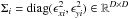 , where ϵi corresponds to the individual measurement errors. Each observation has an associated membership probability vector πi ∈ [0,1] K which relates it to the components of the mixture. Conditioned to the membership probability vector we have
 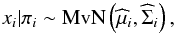 (A.1)where
 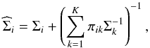 (A.2)and
 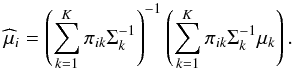 (A.3)We note that each xi is generated by a single multivariate normal distribution, where the natural parameters are weighted averages of the parameters of the individual distributions of the mixture (Heller et al. 2008). The membership probabilities πi are constrained to the simplex1, as done in Gruhl & Erosheva (2014) using the logit or softmax function
 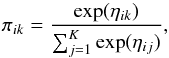 (A.4)where ηi ∈ RK is distributed as a multivariate normal
 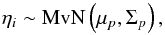 (A.5)with hyperparameters μp ∈ RK−1 and Σp ∈ RK−1 × K−1. To preserve identifiability on the simplex we fix ηiK = 0 ∀i, that is, only K−1 parameters are free. By using a logit multivariate normal prior instead of a typical Dirichlet prior we allow for correlations to exist between individual membership scores (Gruhl & Erosheva 2014), further enhancing the flexibility of the BPM.
In what follows we describe the priors that are used for the variables of the model. We decompose the covariance matrices of the component distributions Σkk ∈ 1,2,3 and of the multivariate prior Σp as 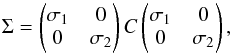 (A.6)where C is a K−1 × K−1 symmetric and positive-definite correlation matrix. For the correlation matrix we use a LKJ prior with one degree of freedom, which corresponds to the uniform distribution for correlation matrices. For the standard deviations a Half-Cauchy prior with a scale parameter γ = 5 is used. The LKJ and Half-Cauchy are standard choices for weakly informative priors. The mean vector of the components is set as defined in Sect. 4. Finally, for μp a normal prior with standard deviation σ = 10 is used. The mean hyperprior of μp is set to (2,1) which translates into to (0.66,0.24,0.09) in the simplex, corresponding to our expectation that the concentration of the bulge is larger than the disk and the disk larger than the cluster.
We are interested in obtaining distributions for the membership vectors, the components covariance, and their respective priors given the data. In traditional Bayesian settings, distributions for the parameters are obtained via approximating the joint posterior of the model using Markov chain Monte Carlo (MCMC) methods. But MCMC scales poorly with high complexity and high dimensionality models, as multi-modality and non-identifiability issues may slow or stall convergence of the chain. Due to this we opt for an optimization approach based on automatic differentiation variational inference ADVI. With ADVI one fits the posterior with a much simpler variational distribution by minimizing their Kullback-Liebler (KL) divergence using gradient-descent based routines. Contrary to expectation-maximization, ADVI is fully Bayesian in the sense that we can draw from the variational posterior and obtain distributions for the parameters rather than point estimates.
The hierarchical model is programmed using the PyMC3 package (Salvatier et al. 2016), which includes an ADVI routine. Because the model is continuous and differentiable on its parameters we can use ADVI straightly. We consider that the procedure has converged when the difference in successive KL divergences is smaller than 0.5%. The results of this procedure are presented in Sect. 6.
All Figures
|
Fig. 1 Color image of chip #15, in pawprint #2 of VVV field b309. The field of view of this image is 12′ × 12′; north Galactic pole is up, positive galactic longitudes are left. |
| In the text | |
|
Fig. 2 Flow chart illustrating the three main steps adopted to computed PMs and explained in detail in the text. |
| In the text | |
|
Fig. 3 CMD for all the stars detected in the field shown in Fig. 1. The hand drawn blue line shows the approximate location of the cluster sequences, while the red and green areas show the bulge RGB and disk MS, respectively. |
| In the text | |
|
Fig. 4 Top: example of PM determination by means of the least square fitting for one of the cluster stars (#98166), with magnitude Ks = 12.4 mag. Each point is the star position in different epochs after been locally-transformed to the reference system of the master catalog. Bottom: CSE in the PM, computed as the error on the slope in the linear fit shown above, as a function of Ks magnitude. The thin red line marks a 3σ clipping on the error distribution; the thick blue line is the median error. Numbers list mean errors in bins of 0.5 mag. The figure inset shows the histogram of errors for 11.5 <Ks< 15 mag before (gray) and after (blue) the 3σ clipping. |
| In the text | |
|
Fig. 5 Left: vector point diagrams for all the stars detected in the field, divided in eight one-magnitude bins according to the CMDs on the right. The green circle shows the adopted membership criterion used to selected cluster members in each magnitude interval. We adopted a radius of 4 mas on the brightest bin and allowed a bigger selection region for poorer measured stars (7.5 at the bottom). Middle: clean CMD for the stars assumed to be cluster members (red points inside the green circle in the VPD). Right: CMD for the field counterpart after excluding likely cluster stars. |
| In the text | |
|
Fig. 6 Hess diagram of the VPD for all the stars with PM CSE lower than 10 mas yr-1. Stars belonging to NGC 6544 cluster in the lower right corner, while field stars are the cloud around zero. This cloud is significantly elongated along the longitude axis, because of the presence of two populations, disk and bulge, with the disk having a significant rotation. |
| In the text | |
|
Fig. 7 Top: CMD showing our selection of RGB bulge stars (red) and main sequence disk stars (blue) after excluding likely cluster members. Bottom: VPD showing the relative PM displacement between the selected stars from the CMD. NGC 6544 stars have been included in green for comparison. |
| In the text | |
|
Fig. 8 PM distribution of bulge and disk stars selected as shown in Fig. 7. Left panels: μlcos(b) distributions. The disk distribution is well fitted with a single Gaussian (black solid line) if the positive tail is excluded. The otherwise better skewed Gaussian fit is shown with a dashed magenta line. The bulge distribution is fitted with two Gaussians, with the centroid of the leftmost one fixed to the value found for the disk. Right panels: μb distributions of bulge and disk are symmetric, allowing a clean fit with one Gaussian. In all panels, centroid and dispersion of the fitted profiles are quoted. |
| In the text | |
|
Fig. 9 Computed orbit for NGC 6544 using an axisymmetric model. The actual location of the cluster is indicated by a red dot while the position of the Sun by a black cross. Blue and black paths show the orbit of the cluster 3 Gyr back and 0.25 Gyr ahead in time, respectively. |
| In the text | |
|
Fig. 10 Upper row: membership probability as a function of magnitude for the bulge, disk and cluster, color coded by point density. The blue and red dashed lines depict the p = 0.66 and p = 0.90 levels used to select likely members of the respective components of the mixture. Middle row: VPD of the whole sample is displayed identically in each panel, color coded by density. The blue and red points stand for subsamples of bulge, disk, and cluster stars selected as those with membership probabilities to the respective component larger than p = 0.66 and p = 0.90 (and with error in their probabilities smaller than 0.35). Lower row: CMD for the most probable members of the bulge, disk and cluster, color coded as above. |
| In the text | |
|
Fig. 11 CMD including only those stars with Pc(i) greater than 70% of being cluster members. The blue solid lines represent the ridge line obtained using VVV data. We adopted a distance modulus of DM0 = 11.96 from Cohen et al. (2014) to match the isochrones from Dartmouth (red) and PGPUC (yellow) databases. The inset shows that, at the level of the SGB-MS, the best fit of the isochrones with the fiducial line is obtained for an age between 11 and 13 Gyr. |
| In the text | |
|
Fig. 12 Galactic coordinate map of the area covered by the tiles b295, b296, b309 and b310. Black points depict the position of likely cluster stars with low PM errors. A color map highlights their surface count density, and a set of contour lines is drawn around the center of NGC 6544. The black and red arrows points toward the Galactic center and along the direction of the cluster orbit, respectively. The cluster center, eccentricity of the outermost contour line, and the angle between its major axis and the Galactic equator are quoted. |
| In the text | |
Current usage metrics show cumulative count of Article Views (full-text article views including HTML views, PDF and ePub downloads, according to the available data) and Abstracts Views on Vision4Press platform.
Data correspond to usage on the plateform after 2015. The current usage metrics is available 48-96 hours after online publication and is updated daily on week days.
Initial download of the metrics may take a while.