| Issue |
A&A
Volume 606, October 2017
|
|
|---|---|---|
| Article Number | A90 | |
| Number of page(s) | 7 | |
| Section | Celestial mechanics and astrometry | |
| DOI | https://doi.org/10.1051/0004-6361/201731544 | |
| Published online | 17 October 2017 | |
Gaia and VLT astrometry of faint stars: Precision of Gaia DR1 positions and updated VLT parallaxes of ultracool dwarfs⋆
1 Main Astronomical Observatory, National Academy of Sciences of the Ukraine, Zabolotnogo 27, 03680 Kyiv, Ukraine
e-mail: This email address is being protected from spambots. You need JavaScript enabled to view it.
2 Space Telescope Science Institute, 3700 San Martin Drive, Baltimore, MD 21218, USA
Received: 10 July 2017
Accepted: 1 August 2017
Abstract
Aims. We compared positions of the Gaia first data release (DR1) secondary data set at its faint limit with CCD positions of stars in 20 fields observed with the Very Large Telescope (VLT) FORS2. We aim at an independent verification of the DR1 astrometric precision taking advantage of the FORS2 position uncertainties which are smaller than one milli-arcsecond (mas).
Methods. In the fields that we observed with FORS2, we projected the Gaia DR1 positions into the CCD plane, performed a polynomial fit between the two sets of matching stars, and carried out statistical analyses of the residuals in positions.
Results. The residual root mean square (rms) roughly matches the expectations given by the Gaia DR1 uncertainties, where we identified three regimes in terms of Gaia DR1 precision: for G ≃ 17−20 stars we found that the formal DR1 position uncertainties of stars with DR1 precisions in the range of 0.5–5 mas are underestimated by 63 ± 5%, whereas the DR1 uncertainties of stars in the range 7−10 mas are overestimated by a factor of two. For the best-measured and generally brighter G ≃ 16−18 stars with DR1 positional uncertainties of <0.5 mas, we detected 0.44 ± 0.13 mas excess noise in the residual rms, whose origin could be in both FORS2 and Gaia DR1. By adopting Gaia DR1 as the absolute reference frame, we refined the pixel scale determination of FORS2,leading to minor updates to the parallaxes of 20 ultracool dwarfs that we published previously. We also updated the FORS2 absolute parallax of the Luhman 16 binary brown dwarf system to 501.42 ± 0.11 mas.
Key words: astrometry / methods: data analysis / surveys / catalogs / parallaxes / stars: individual: WISE J104915.57 / 531906.1
Based on observations made with ESO telescopes at the La Silla Paranal Observatory under programme IDs 086.C-0680, 087.C-0567, 088.C-0679, 089.C-0397, and 090.C-0786.
© ESO, 2017
1. Introduction
Gaia’s first data release (DR1) provides accurate astrometric and photometric data for about one billion stars in the magnitude range G ≃ 3−20.7 (Gaia Collaboration 2016a,b). Independently of the mission’s own validation effort (Arenou et al. 2017), several studies have found generally excellent agreement between external measurements and parallaxes (e.g. Gaia Collaboration 2017; Casertano et al. 2017) and proper motions (e.g. van der Marel & Sahlmann 2016; Watkins & van der Marel 2017) of bright stars in the Gaia DR1 primary data set (Lindegren et al. 2016). The bulk content of DR1, however, is the secondary data set of generally fainter stars for which it lists stellar positions at the epoch 2015, but no parallax or proper motions.
The DR1 positions were tested with numerous methods, including the comparison with external catalogues of sufficient precision (Arenou et al. 2017). The external validation of the astrometric accuracy of positions was made with two catalogues:the First U.S. Naval Observatory Astrometric Robotic Telescope (URAT1) catalogue (Zacharias et al. 2015) with a precision of positions 10–30 milli-arcsecond (mas), and with positions of quasars inthe International Celestial Reference Frame (ICRF2) catalogue of quasi-stellar objects (Fey et al. 2015), and no deviations from the model of uncertainties adopted in DR1 were found.
Mignard et al. (2016) compared ICRF2 positions (Ma et al. 2009; Fey et al. 2015) of G = 16−20 sources with the auxiliary quasar table of DR1. They reported that if a comparison is made with the secondary data set of DR1, the dispersion of the normalised coordinate differences is about 30% higher than expected for the defining ICRF2 sources, probably because the positional uncertainties in DR1 are underestimated.
So far, no other validation of the DR1 secondary data set astrometry has been made at the mas-level because most external catalogues have insufficient accuracy. Here, we address this issue using CCD astrometric data sets obtained with the Focal Reducer and low dispersion Spectrograph 2 (FORS2) camera installed at the Very Large Telescope (VLT) as described by Lazorenko et al. (2014a). Our ground-based astrometry has a typical precision of 0.1–0.5 mas for individual stars. Comparison with DR1 is made by projecting its star positions into CCD space, computing the residuals of positions, and performing the statistical analysis of the scatter of these residuals. This investigation concerns only the random component of astrometric errors, because FORS2 astrometry is inherently differential and is applied to G ≃ 16−20 stars that are towards the faint end of the DR1 secondary data set. We also better characterise the distortion of the FORS2 camera, which allows us to re-calibrate the pixel scale and to update the parallaxes of ultracool dwarfs observed in our programmes.
2. Differential CCD data sets of FORS2 field stars
In 2010 we started an astrometric planet search targeting 20 ultracool dwarfs and very low-mass stars (Sahlmann et al. 2014, 2015a,b). Observations were obtained with the FORS2/VLT camera (Appenzeller et al. 1998), whose focal plane is composed of two CCD chips.Images obtained with the high-resolution collimator have an approximate pixel scale of s0 = 0.1261″/px (Lazorenko et al. 2014a). Our observations’ design and reduction methods reach precisions of ~0.05−0.07 mas for I = 15−17 mag stars (Lazorenko et al. 2009, 2014a). Our CCD data setbased on observations in 2010–2013 contains images of I ≃ 16−22 mag stars in 20 fields close to the southern galactic plane, each covering ~ 4′ × 4′. The list of fields with a numbering adopted in Lazorenko et al. (2014a) is given in Table 1.
Sky fields,root mean square (rms) of the positional differences between DR1 and FORS2 data sets, and average values of σG and σF for chip1.
The main application of this data set is the search for reflex motion of the targets measured relative tothe fieldstars in the plane of the sky. To ensure the best elimination of the atmospheric image motion and optical distortion of the telescope, the positions of the targets were computed relative to a reference frame formed by the dense grid of reference stars. The reference areas are circular and centred on the target. The reduction within each individual CCD image was made using a polynomial model with M = (n + 1)(n + 2)/2 basic functions per each CCD axis, which include full two-dimensional polynomials of x, y with the maximum power n, removing in this way the most important low-frequency components of the image motion spectrum (Lazorenko et al. 2009). Besides the reduction within the CCD plane, this model also takes into account the change of positions due to the proper motion, parallax, and colour effects.
2.1. RF data set of FORS2 field stars
A first supplementary result of the programme are the astrometric parameters of every star measured relative to the reference frame centred on the target ultracool dwarf: CCD positions x, y for the epoch 2011.38, proper motions in the CCD system, parallaxes, and chromatic parameters. The precision of our stellar positions σF ~ 0.1−1 mas is comparable to that of Gaia DR1 secondary data set, which is 0.1−20 mas (Gaia Collaboration 2016a), so we use the results of the n = 4 (M = 15) reduction for the current investigation. We will refer to it as the reference frame (RF) data set and it contains 6208 stars in 20 fields. There are two sub-sets, one per CCD chip.
The argumentation in the next sections relies on the fact that the system of these astrometric parameters is strictly homogeneous because it is defined by the samereference frame and basic functions.It means that for each RF star the differential x, y and the “absolute” xabs, yabs positions in some external catalogue given in the ICRF system, for example Gaia, are related by the expression  (1)along the X axis (the equivalent equation holds for the Y axis), wherexF = −s0(x−xdwarf) are the FORS2 positions expressed in units of arc and measured relative to the approximate position xdwarf of the target, and Fn(x−xdwarf,y−ydwarf) is a sum of M two-dimensional basic functions of the maximum power n, with free model coefficients, which describe the transformationbetween the local reference frames in some sky fields and Gaia (Lazorenko et al. 2009). The term Fnoise models random noise that is not correlated across the field. The variance of Fnoise is equal to the quadratic sum of σF and the positional uncertainty in the external catalogue.
2.2. FOV data set of FORS2 field stars
A second result of these FORS2 observations is the astrometric parameters of stars obtained also with n = 4, but in a slightly different way. Specifically, each star was reduced with its own circular reference area. Therefore the locations of the reference frames are not fixed and move in the CCD plane. These individual areas cover the whole field of view (FOV) of the CCD and therefore we will refer to them as the FOV data set.
The system of astrometric parameters in the FOV data set is not exactly homogeneous because the set of reference stars is different for every star, thus we are using multiple reference frames. In comparison to RF, the FOV data set is larger and contains about 12 000 stars, because it includes stars outside the central reference areas aligned to the programme targets. These data were converted to the ICRF system using the US Naval Observatory (USNO-B) catalogue (Monet et al. 2003) and are available in the Strasbourg astronomical Data Center(Lazorenko et al. 2014b) as a deep catalogue of positions, proper motions, and parallaxes of faint stars in 20 sky fields. Because that conversion was based on USNO-B, the absolute precision of the astrometry degraded to ~0.2′′, which is insufficient for a comparison with Gaia DR1. Therefore, to take advantage of the sub-mas precision of FORS2 differential astrometry, we instead used the original CCD positions and proper motions of FOV stars set by the reference frame fixed to the CCD pixels.
Both FORS2 data sets are based on exactly the same measured photocentres of star images and an identical reduction method, but differ in the reference frame definition. Although this difference may appear subtle, the discussion in Sect. 3 demonstrates that the RF positions are in better agreement with Gaia. We present the analysis of both data sets because the FOV data set has twice as many stars and therefore allows for a more robust comparison with DR1 positions.
3. Data analysis
We compared the positions of stars in Gaia DR1 that are in common with the RF and FOV data sets, which were converted from their average epoch2011.5–2012.1 to the Gaia DR1 epoch 2015.0 using the proper motions measured with FORS2. These FORS2 positions refer to the barycentre of the solar system, because the proper motions and parallaxes were accounted for and atmospheric chromaticity parameters were incorporated into the astrometric model. The position uncertainties σF in 2015 were computed using the uncertainty and covariance matrix of the astrometric parameters of FORS2 stars, and include input from all known types of errors. The average value of σF over all sky fields is given in Table 1. Because the proper motions of FORS2 catalogues were obtained with a short timebase of about two years, the conversion between epochs significantly degraded the precision of FORS2 positions. For example, the typical precision for bright stars is roughly 0.1 mas for positions and 0.07−0.15 mas/yr for proper motions. After conversion to 2015, the proper motion errors propagated for a three and a half years difference increase the uncertainty of positions four-fold, to about 0.4 mas.
3.1. Error budget and unbiased rms of the residuals
We define the residuals, for example along the X axis, between FORS2 xF and DR1 positions xabs computed as a tangent projection to the CCD plane, as Δ = xF−xabs that indicates the left side of Eq. (1). The expected variance of the residuals is modelled by the sum  , which includes the formal uncertainty σG of DR1 and the uncertainty σF of FORS2 positions at 2015. The average value of σF is 0.64 mas and small or comparable to σG for stars cross-identified with DR1. It is reasonable to assume that the measured variance of Δ can deviate from this model, and a more realistic error budget is
  (2)where we introduced an additional noise component ν to balance the discrepancy between the observed rms of the residuals and the nominal uncertainties in the catalogues. The ν component may be related to Gaia DR1 or FORS2 or both.
The problem is that the residuals Δ cannot be measured directly because xF and xabs are related by the polynomial relation in Eq. (1). While xabs represents a flat coordinate system, the FORS2 positions xF are affected by high-order geometric distortion. We therefore considered the corrected position residuals and the corrected residual rms. The corrections are based on the fact that the unbiased variance of the residuals  computed with the least squares fit of i = 1...N measurementsper axis for N common stars is
  , where M is the number of fit parameters and wi are the weights which depend on a factor (e.g. on σG). For a limited sub-sample of N′<N residuals in a narrow range of σG where the wi are approximately constant, the unbiased estimate of the variance is
  , where the angle brackets denote an average taken over N′ measurements. Therefore the unbiased estimate of the residual rms is
  where
where  is a factor that compensates for the decrease in the degrees of freedom.
The original residuals Δ are affected by the least squares fit and cannot be restored exactly. However, they can be approximated by the corrected residuals  with an unbiased variance. In the following discussion we deal with the bias-corrected rms and residuals Δ defined in this way.
3.2. Individual residuals between DR1 and FORS2
Equatorial star positions of DR1 stars were converted to Cartesian coordinates in the CCD plane using a tangent-plane projection. The reference point of the projection corresponded to the position of target objects, that is to the geometric centres of the RF data sets.Then we proceeded with stars whose uncertainty σG is better than 20 mas, cross-identified DR1 and FORS2 stars, and applied the polynomial model (Eq. (1)) to transform between these two sets of positions. The data for FORS2 chip1 and chip2 were reduced separately because the relative offset and orientation between the chips are known only approximately. Cross-matching between catalogues consisted in the initial rough identificationof stars in a 1′′ window and three iteration cycles of fitting the residuals Δ by polynomial functions of degree n = 3 and rejection of outliers over 60 mas. With two concluding iterations, detailed below, we obtained the final identification and derived the residuals Δ.
The main parameters of the fitting procedure are shown in Table 1. We present parameters for chip1 only because those for chip2 are similar, except for a smaller star number N and polynomial degree n. For every field and chip we had to choose the optimal polynomial degree n with number M of fit parameters. Naturally, an increase of M will lead to smaller residuals because there are more free parameters. Fitting polynomials with an arbitrarily high degree is undesirable and it is therefore necessary to identify the highest M for a particular data set. Since our model is linear and the errors are reasonably well-behaved, we used the F-test of additional model parameters,which yields the probability that the simpler model is true. This approach is described in detail by Sahlmann (2017) who applied it to the comparison between Gaia DR1 and Hubble Space Telescope (HST) observations of the James Webb Space Telescope (JWST) calibration field.
The weights in the system Eq. (1) of the transformation of FORS2 to DR1 were set to  initially computed with ν = 0, which therefore assumes that the uncertainties σG and σF are good estimates. The stars were considered identified when the residuals in positions were within 5σΔ. Still, many stars were rejected as outliers because their residuals were slightly above the adopted five-sigma limit. The unusually high rate of outliers detected at this phase of identification, especially for stars with σG< 1 mas, indicates that the distribution of the residuals deviates from prediction (2). To obtain a more stable identification and to find a reasonable compromise between the number of identified stars and the rms of the residuals, we therefore computed the final weights in most fields with different values of ν = [0,0.7,1] mas.
3.3. rms of the residuals
The number of stars cross-identified with the RF and FOV data sets is 1421 and 3705, respectively, and the residual scatter is smaller for the comparison of DR1 with RF. To illustrate the statistics of the residuals, we computed for every field and FORS2 chip the rms of the residuals Δ and the (quadratic) average value of ⟨ σG ⟩ (see Table 1). These values are visualised in Fig. 1 and show an approximately linear correlation at 2 < ⟨ σG ⟩ < 5 mas where σG dominates over the other error components, including the FORS2 noise σF that has an amplitude below 1 mas (Table 1).
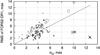 |
Fig. 1 Average rms of the residuals Δ between DR1 and FORS2 data sets FOV (open circles) and RF (grey circles) versus average value of σG for each sky field (field No. 20 marked by crosses) and each chip.The circle size is proportional to the number of stars, from 11 to 285. |
The rms is systematically higher for the residuals between DR1 and FOV in comparison to the residuals between the DR1 and RF data set, which is due to the difference of their construction as discussed in Sect. 2.2. We note that field No. 20 has unexpectedly small residuals at large σG.
We investigated how well the measured rms matches the model precision σΔ along a full range of σG = 0...20 mas. For this purpose the residuals FORS2−DR1 were binned in 1 mas intervals of σG and quadratically averaged separately for every field and chip. The results presented in Fig. 2 demonstrate significant deviations from the model dependence Eq. (2) computed with ν = 0 and shown by the dashed line, especially for σG< 0.5 mas. In that region, associated with brighter stars, σG and σF are much smaller than the measured rms values. This allowed us to derive a reliable estimate of ν by fitting the excess in rms with the expression (2). In this way we obtained ν = 2.04 ± 0.11 mas for the comparison of DR1 with FOV and ν = 0.66 ± 0.08 mas for the comparison of DR1 with RF. The significantly smaller excess ν in the latter case is a consequence of the more homogeneous astrometric system of the RF data set. The error component ν could be due to unaccounted excess noise in either DR1 or FORS2 astrometry, and the smaller value of 0.66 ± 0.08 mas can be put forward as an upper limit of ν potentially related to DR1. This estimate is strictly valid only for stars with G-band photometric magnitudes of 16.0–17.5, and average values of σG ≃ 0.31 mas and σF ≃ 0.38 mas. The value ν = 2.04 mas obtained from the comparison of DR1 with FOV is likely caused by noise related to the multiple reference frames used in the compilation of the FOV data set (Sect. 2.2).
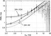 |
Fig. 2 rms of the positional residuals Δ between DR1 and FOV and between DR1 and RF for chip1 (circles) and chip2 (triangles) in every 1 mas bin of σG. Three-sigma error bars are drawn under the assumption of a normal error distribution. These data are compared with the model uncertainty σΔ computed with ν = 0 in Eq. (2) (dashed lines) and with a value of ν that fits the rms at σG < 0.5 mas (dashed-dotted lines). Solid lines show the fit function Eq. (3). |
Since we determined the value of ν, Eq. (2) is fully defined in the range of σG and for any star sample we can compute σΔ, which models the expected value of the rms. The functional dependence of σΔ on σGis shown by the dashed-dotted lines in Fig. 2. The measured rms values now are well fitted with the model at σG < 1 mas. However, at σG = 1−5 mas we note a systematic positive bias of about a factor of 1.5, which remains constant in the logarithmic scale of the plot. Figure 2 suggests that the model (2) is not adequate in the σG = 1−10 mas range because here we found rms > σΔ. In this interval, σG is much larger than the other noise components in Eq. (2), including ν and σF, which typically are 0.5–0.7 mas. Therefore, the discrepancy with the observations is likely due to an underestimated variance  . We laid out the improved error budget
 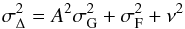 (3)with an additional parameter A that modulates the DR1 uncertainties.The two cases, A> 1 and A < 1 indicate that σG is under- and over-estimated, respectively. We fitted the complete sample of all residuals with this model, where we ingested both data sets of FORS2 and used three fit parameters: νFOV for the residuals “DR1”-“FOV”, νRF for the residuals “DR1”-“RF”, and A as a common parameter. The data were fit in the σG range 0−5.5 mas and produced the model parameters νFOV = 2.13 ± 0.09 mas, νRF = 0.44 ± 0.13 mas, close to the previous estimate, and A = 1.63 ± 0.05. The fit approximates the observed data well for σG< 5 mas. At larger σG in the interval of 7–20 mas, the measured rms reaches a ceiling of about 5–8 mas, therefore Eq. (3) is not applicable there.
The solution of Eq. (3) differs between data sets in the range of σG< 1 mas because there σF is comparable to σG. We fit the observed rms in this region separately for both FORS2 data sets but obtained similar solutions for A. Therefore, we fit the combined (FOV and RF) data set with Eq. (3) and obtained A = 1.83 ± 0.07, similar to the above result obtained in a wider range of σG. It means that Eq. (3) is applicable at least within a range of 0.5 <σG< 5 mas and our results suggest that in this region the uncertainties of the DR1 secondary data set are underestimated.
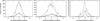 |
Fig. 3 Distribution of the normalised position residuals Δ between DR1 and RF (solid curves) and between DR1 and FOV (dashed curves) for stars with 1 <σG < 5 mas.Left panel: the normalisation is based on σΔ computed with A = 1.63; middle panel: the same with A = 1; right panel: the same for stars with σG> 7 mas assuming that A = 1. The corresponding Gaussian distributions are shown by dotted lines. |
We studied whether there is a difference in the residual rms for stars with large and small astrometric excess noise ε, which indicates the quality of the astrometric fit for every star in DR1 (Lindegren et al. 2016). The stars were divided into two groups with “large” and “small” ε as defined by a threshold value. Using different thresholds from 0.5 to 2 mas, we found no clear difference in the rms value for the subsets of stars, partly due to the small number of stars with large ε.
We found that Eq. (3) fits well the measured rms in every field, except for field No. 20 with an rms significantly below σΔ and three to five times smaller than σG. This field is unusual in terms of the stellar brightness and σG distributions. Whereas in most fields only ~10% of stars have σG values of 10−20 mas, about half of the stars in field No. 20 have such large uncertainties. This is despite the fact that those stars are relatively bright (G ≃ 17−19) and should therefore have σG ≃ 0.5−2 mas as typical in the other fields. The reason for this peculiarity may be that Gaia observed this field less often, as reported by the average number of good CCD observations in DR1 (catalogue entry astrometric_n_good_obs_al), which is smaller than for the other fields. Our findings therefore may demonstrate variations of the DR1 uncertainties in different areas in the sky.
3.4. Distribution of the residuals
The position residuals contain information on the distribution of DR1 errors, which can deviate from the normal law. Figure 3 shows the observed distribution of the residuals between FORS2 data sets and DR1 normalized to σΔ computed with the derived fit parameters. Because the uncertainty σΔ is correctly modelled by Eq. (3) only within a limited range of σG, we generated the histograms for stars in a conservative 1 <σG< 5 mas range. We rejected residuals with large correction factors γ> 1.3, a situation usually related to sky fields with an insufficient number of identified stars N. The derived distributions follow a Gaussian distribution with no excess in the wings.
To demonstrate how the distribution shape depends on the value of A, we computed the uncertainties σΔ with A = 1 (that is, using the original uncertainties of DR1) and obtained the distributions in the middle panel of Fig. 3 with the best-fit estimates of νFOV and νRF. The difference relative to the left panel demonstrates the effect of the bias in the σΔ. Finally, we obtained the residual distribution for stars with σG> 7 mas (right panel). The strong concentration at zero indicates an overestimation of σG by at least a factor of two, as is also seen in Fig. 2.
3.5. Discussion
It is unlikely that the entirety of these results can be caused by errors in the FORS2 astrometry. For instance, excess noise ν can also originate if σG is correct but instead our value of σF is underestimated. For stars with σG < 1 mas the average value of σF is 0.41 mas. Increasing this value quadratically by ν = 0.44 mas yields a new estimate of σF = 0.73 mas (78% over its nominal value), which removes the discrepancy between the measured and model variance of the residuals FORS2−DR1, while keeping σG untouched in this range. In this scenario, because σF is dominated by the uncertainty in proper motion, the 78% excess in our errors would refer almost entirely to FORS2 proper motions. However, applying the same argument in the range of σG > 1 mas, the excess noise ν cannot be due to underestimated FORS2 errors because that would lead to unrealistic manifold corrections to σF.
Potential sources of unaccounted noise in FORS2 positions are systematic errors in the measured photocentres of stars caused by imperfect modelling of the point spread function or from unmodelled blended light from nearby stars. We investigated other potential sources of the excess noise by looking for correlations between the residuals and brightness, position on the CCD, proper motion, and chromaticity parameters of individual stars. We did not find any significant correlation.
4. Update of the FORS2 pixel scale
The conversion of relative to absolute positions on the basis of Gaia DR1 allows us to derive the coefficients of the function Fn(x−xdwarf,y−ydwarf), which determine the optical distortions of the FORS2 camera, the perpendicularity of the CCD axes, the pixel scale and its variation across the CCD, and the differences of scales along X and Y directions. It is convenient to present Eq. (1) in the conventional form s0x′−xG = ax′ + by′ + x′0 + ... and s0y′−yG = cx′ + dy′ + y′0 + ..., where x′ = −(x−xdwarf), y′ = y−ydwarf, and the high-order terms of the function Fn were omitted. Here we define the scale s and the coefficients of geometric distortion as  (4)where sx−sy characterises the scale difference between the two axes and the skew term gives information on the non-perpendicularity of those axes. Above expressions are applicable at the location of the target, where x′ = y′ = 0.In general, s(x,y) and the other distortion coefficients are functions of field location and can be computed from the partial derivatives of Fn including the higher order terms (Sahlmann 2017).
Pixel scales, the skew and rotation parameters, and updated ultracool dwarf parallaxes ϖ.
The values of s for each sky field at the position of the target x = xdwarf, y = ydwarf are given in Table 2 both for RF and FOV data sets. For comparison, the table contains scales s0, which were previously derived on the basis of the USNO-B catalogue (Lazorenko et al. 2014a). Those scales were smaller than sFOV and sRF. This underestimation of the pixel scale was caused by the small degree of the polynomial transformation Fn that we used in Lazorenko et al. (2014a) that was fixed to n = 3 for all fields, but did not carry the x2y and xy2 terms because of the insufficient precision of USNO-B. Function Fn allowed for the transformation to ICRF with a precision of 40–70 mas, however, the absence of the x2y, xy2, and higher-order terms prevented it from resolving the field distortion. This is evident in Fig. 4, which shows how the scale s(x,y) changes along the X axis of chip1 at Y = 100 px, close to the chip gap. The figure corresponds to the FOV data set, but it is nearly the same for the RF set. The function s(x,y) is symmetric and reaches a maximum value of 126.33 mas at the chip centre (column X = 1000 px). The use of a simpler transformation Fn broadened the peak of s(x,y) and yielded the lower value of 126.1 mas reported in Lazorenko et al. (2014a).
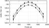 |
Fig. 4 Change of FORS2 pixel scale s in chip1 along the X axis for each sky field at Y = 100 px (open circles) and at Y = 500 px (crosses). The average scales (solid curves), the scale obtained by Lazorenko et al. (2014a, horizontal dashed line),and the scale s computed with use of distortion coefficients in chip 2 at Y = 0 (dotted curve) are shown. |
The function Fn represents the difference between the local reference frame and Gaia, but not directly between the star positions in the CCD system and Gaia. This induces additional distortions in the differences x−xdwarf and y−ydwarf and is the reason why the individual values of s are scattered by over three sigma (see Table 2). In particular, the scatter of points in Fig. 4 is due to this effect. Figure 4 shows that the scale changes across the chip and in the outer regions of Y = 500 px are about 0.5 mas/px lower compared to at Y = 100 px. This confirms that the conversion from pixel to angular units should be done with a scale evaluated at the position x = xdwarf, y = ydwarf of the target. In our observations xdwarf and ydwarf varied by ~ 100 pixels for different targets, thus adding additional scatter in the measured scale (Table 2) because that is a function s(x,y).
The pixel scales in chip 1 and chip 2 of FORS2 cannot be directly compared because they are modulated by the optical distortion. To investigate possible scale differences between chips, we used the coefficients of Fn of chip 2 and computed s(x,y) at the dividing gap between the chips, where Fn is still applicable. These scales correspond to Y = 0 in chip 1 (dottedcurve in Fig. 4) and are in good agreement with scales at the nearby location defined by Y = 100 px. Attributing the common curved shape to the optical distortion and the offset to the separation in Y, we find no scale discontinuity between the two chips.
The skew parameter given in Table 2 shows that the axes’ non-perpendicularity is small (0.01–0.02 mas/px) and consistent with zero. However, it formally varies by over three sigma between the sky fields due to the skew of the local reference frames.The difference sx−sy shows a similar random scatter with an average close to zero. This disagrees with our former estimate of −0.37 ± 0.06 mas/px (Lazorenko et al. 2014a), possibly for a reason similar to the discussed difference of the pixel scale.
The Flexible Image Transport System (FITS) headers of FORS2 indicate a relative rotation of 0.083° between the two CCD chips. We verified this by evaluating the coefficients of the function Fn. For chip 1, we find the inclination θ1 = (b−c)/2 between the ICRF and the axes of the FOV reference frames at the position of the target, which approximately corresponds to the inclination between the ICRF and the CCD axes. We used the function Fn for chip 2 to determine the inclination θ2 about 200 px below the target. Instead of b and c we used their exact local values computed with the partial derivatives of Fn. The difference θ1−θ2 between the inclination angles is the rotation between the chips, which is given in Table 2 for each field. Its median value is (0.202 ± 0.016) mas/px, thus the Y axis of chip 1 is rotated clock-wise relative to that of chip 2. This corresponds to a rotation of (0.092 ± 0.009)° and agrees with the value given in the FITS headers.
5. Updated parallaxes of ultracool dwarfs
With the now better-determined pixel scales, we corrected the (absolute) parallaxes ϖ0 of 20 ultracool dwarfs reported in Sahlmann et al. (2014) that were computed with scales s0 given in Table 2 by applying a multiplicative factor β = s/s0. We used scales obtained in individual sky fields to take into account variations related to the local reference frames. We used s = sRF because of the better internal precision, but the factors β computedwith s = sFOV are nearly the same. The applied β factors vary from 0.9990 to 1.0028, thus the corrections are small and change the parallaxes ϖ by about 0.1 mas, comparable to the formal parallax uncertainties.
The effect is more significant for the binary brown dwarf WISE J104915.57−531906.1 (LUH16, Luhman 2013). By analysing the FORS2 images obtained by Boffin et al. (2014) we derived the relative (500.23′′) and absolute parallax ϖ = 500.51 ± 0.11 mas of this system located ~2 pc from the Sun (Sahlmann & Lazorenko 2015). Using HST observations in 2014–2016, a pixel scale determined on the basis of Gaia DR1, and the parallax correction of Sahlmann & Lazorenko (2015),Bedin et al. (2017) derived the relative and absolute parallax of LUH16 of 501.118 mas and 501.398 ± 0.093 mas, respectively, significantly larger than the values of Sahlmann & Lazorenko (2015). Applying the correction factor β computed with s0 = 126.1 mas from Sahlmann & Lazorenko (2015) and s = 126.329 ± 0.010 mas, which is the median of the complete set of sFOV and sRF, we obtained the updated relative 501.139 mas and absolute ϖ = 501.419 ± 0.11 mas FORS2 parallax of LUH16, in agreement with Bedin et al. (2017).
6. Conclusion
We compared the predicted and measured residual rms in position between the Gaia DR1 and FORS2 astrometric data sets of 20 astrometric fields. The relationships between these two data sets are non-trivial and require the introduction of an auxiliary term ν to take into account the excess in the residual scatter. In addition, the behaviour depends on the Gaia position uncertainty σG and is different in the ranges smaller than 5 mas and larger than 7 mas. Our study is sensitive to the random component of position errors that are uncorrelated on spatial scales of about 2−4′ because of the limitations of the FORS2 differential astrometry. Our results apply to the faint end of the Gaia DR1 content, that is to stars with G> 16.
In the range of σG = 0.5−5 mas, our results suggest that the actual value of the DR1 uncertainty is underestimated by 63% for 80% of stars typically fainter than G = 17. This conclusion agrees with the finding of Mignard et al. (2016, Appendix A), on
the uncertainty of the Gaia DR1 secondary data set. In contrast, we find that for σG> 7 mas, that is mostly G> 20 stars, the actual DR1 uncertainties are overestimated by a factor of two.
The excess noise ν in our model was detected primarily in the residual rms of G = 16−18 stars with σG< 0.5 mas. This noise could originate from Gaia DR1 and/or from FORS2. We cannot pinpoint the likely source, but we determined that the component related to Gaia DR1 cannot exceed 0.44 ± 0.13 mas, which corresponds to νRF for the RF data set. We expect that the situation will be clarified with the second Gaia data release that will provide us with astrometry of even higher quality.
Finally, the availability of the Gaia astrometry allowed us to more precisely calibrate the geometric distortions of our extensive FORS2 data sets, to derive a better pixel scale, and consequently update the parallaxes of the 20 ultracool dwarfs in our planet search programme and that of the LUH16 binary. Whereas for most of our targets the correction is smaller than 0.1 mas, the updated FORS2 parallax of the LUH16 system is larger by about 1 mas.This demonstrates the value of the accurate, optically faint, and dense reference frame that Gaia provides for high-precision ground-based differential astrometry.
Acknowledgments
This work has made use of data from the ESA space mission Gaia (http://www.cosmos.esa.int/gaia), processed by the Gaia Data Processing and Analysis Consortium (DPAC, http://www.cosmos.esa.int/web/gaia/dpac/consortium). Funding for the DPAC has been provided by national institutions, in particular the institutions participating in the Gaia Multilateral Agreement.
References
- Appenzeller, I., Fricke, K., Fürtig, W., et al. 1998, The Messenger, 94, 1 [NASA ADS] [Google Scholar]
- Arenou, F., Luri, X., Babusiaux, C., et al. 2017, A&A, 599, A50 [NASA ADS] [CrossRef] [EDP Sciences] [Google Scholar]
- Bedin, L. R., Pourbaix, D., Apai, D., et al. 2017, MNRAS, 470, 1140 [NASA ADS] [CrossRef] [Google Scholar]
- Boffin, H. M. J., Pourbaix, D., Mužić, K., et al. 2014, A&A, 561, L4 [NASA ADS] [CrossRef] [EDP Sciences] [Google Scholar]
- Casertano, S., Riess, A. G., Bucciarelli, B., & Lattanzi, M. G. 2017, A&A, 599, A67 [NASA ADS] [CrossRef] [EDP Sciences] [Google Scholar]
- Fey, A. L., Gordon, D., Jacobs, C. S., et al. 2015, AJ, 150, 58 [NASA ADS] [CrossRef] [Google Scholar]
- Gaia Collaboration (Brown, A. G. A., et al.) 2016a, A&A, 595, A2 [NASA ADS] [CrossRef] [EDP Sciences] [Google Scholar]
- Gaia Collaboration (Prusti, T., et al.) 2016b, A&A, 595, A1 [NASA ADS] [CrossRef] [EDP Sciences] [Google Scholar]
- Gaia Collaboration (Clementini, G., et al.) 2017, A&A, 605, A79 [NASA ADS] [CrossRef] [EDP Sciences] [Google Scholar]
- Lazorenko, P. F., Mayor, M., Dominik, M., et al. 2009, A&A, 505, 903 [NASA ADS] [CrossRef] [EDP Sciences] [Google Scholar]
- Lazorenko, P. F., Sahlmann, J., Ségransan, D., et al. 2014a, A&A, 565, A21 [NASA ADS] [CrossRef] [EDP Sciences] [Google Scholar]
- Lazorenko, P. F., Sahlmann, J., Ségransan, D., et al. 2014b, VizieR Online Data Catalog: J/A+A/565/A21 [Google Scholar]
- Lindegren, L., Lammers, U., Bastian, U., et al. 2016, A&A, 595, A4 [NASA ADS] [CrossRef] [EDP Sciences] [Google Scholar]
- Luhman, K. L. 2013, ApJ, 767, L1 [NASA ADS] [CrossRef] [Google Scholar]
- Ma, C., Arias, E. F., Bianco, G., et al. 2009, IERS Technical Note, 35 [Google Scholar]
- Mignard, F., Klioner, S., Lindegren, L., et al. 2016, A&A, 595, A5 [NASA ADS] [CrossRef] [EDP Sciences] [Google Scholar]
- Monet, D. G., Levine, S. E., Canzian, B., et al. 2003, AJ, 125, 984 [NASA ADS] [CrossRef] [Google Scholar]
- Sahlmann, J. 2017, Astrometric accuracy of the JWST calibration field catalog examined with the first Gaia data release, Analysis Report JWST-STScI-005492, STScI [Google Scholar]
- Sahlmann, J., & Lazorenko, P. F. 2015, MNRAS, 453, L103 [NASA ADS] [CrossRef] [Google Scholar]
- Sahlmann, J., Lazorenko, P. F., Ségransan, D., et al. 2014, A&A, 565, A20 [NASA ADS] [CrossRef] [EDP Sciences] [Google Scholar]
- Sahlmann, J., Burgasser, A. J., Martín, E. L., et al. 2015a, A&A, 579, A61 [NASA ADS] [CrossRef] [EDP Sciences] [Google Scholar]
- Sahlmann, J., Lazorenko, P. F., Ségransan, D., et al. 2015b, A&A, 577, A15 [NASA ADS] [CrossRef] [EDP Sciences] [Google Scholar]
- van der Marel, R. P., & Sahlmann, J. 2016, ApJ, 832, L23 [CrossRef] [Google Scholar]
- Watkins, L. L., & van der Marel, R. P. 2017, ApJ, 839, 89 [NASA ADS] [CrossRef] [Google Scholar]
- Zacharias, N., Finch, C., Subasavage, J., et al. 2015, AJ, 150, 101 [NASA ADS] [CrossRef] [Google Scholar]
All Tables
Sky fields,root mean square (rms) of the positional differences between DR1 and FORS2 data sets, and average values of σG and σF for chip1.
Pixel scales, the skew and rotation parameters, and updated ultracool dwarf parallaxes ϖ.
All Figures
|
Fig. 1 Average rms of the residuals Δ between DR1 and FORS2 data sets FOV (open circles) and RF (grey circles) versus average value of σG for each sky field (field No. 20 marked by crosses) and each chip.The circle size is proportional to the number of stars, from 11 to 285. |
| In the text | |
|
Fig. 2 rms of the positional residuals Δ between DR1 and FOV and between DR1 and RF for chip1 (circles) and chip2 (triangles) in every 1 mas bin of σG. Three-sigma error bars are drawn under the assumption of a normal error distribution. These data are compared with the model uncertainty σΔ computed with ν = 0 in Eq. (2) (dashed lines) and with a value of ν that fits the rms at σG < 0.5 mas (dashed-dotted lines). Solid lines show the fit function Eq. (3). |
| In the text | |
|
Fig. 3 Distribution of the normalised position residuals Δ between DR1 and RF (solid curves) and between DR1 and FOV (dashed curves) for stars with 1 <σG < 5 mas.Left panel: the normalisation is based on σΔ computed with A = 1.63; middle panel: the same with A = 1; right panel: the same for stars with σG> 7 mas assuming that A = 1. The corresponding Gaussian distributions are shown by dotted lines. |
| In the text | |
|
Fig. 4 Change of FORS2 pixel scale s in chip1 along the X axis for each sky field at Y = 100 px (open circles) and at Y = 500 px (crosses). The average scales (solid curves), the scale obtained by Lazorenko et al. (2014a, horizontal dashed line),and the scale s computed with use of distortion coefficients in chip 2 at Y = 0 (dotted curve) are shown. |
| In the text | |
Current usage metrics show cumulative count of Article Views (full-text article views including HTML views, PDF and ePub downloads, according to the available data) and Abstracts Views on Vision4Press platform.
Data correspond to usage on the plateform after 2015. The current usage metrics is available 48-96 hours after online publication and is updated daily on week days.
Initial download of the metrics may take a while.