© The Authors 2024

1 Introduction

High-precision relative astrometry is a powerful technique used to study the dynamics of various stellar objects, particularly those near the Galactic center (it also has many other astrophysical applications not discussed in this paper). For these purposes, the astrometric precision required should be of 10–100 μas or better. For bright objects, this requirement has been well realized with the space mission Gaia (Lindegren et al. 2021). However, because space telescopes are limited in the size of their light collecting areas, faint objects are measured with a lower accuracy.

The new generation of extremely large ground-based telescopes with apertures of about 40 m and adaptive optics have a diffraction-limited resolution, and they can measure very faint stars with a good accuracy. For the Extremely Large Telescope (ELT) (Pott et al. 2018; Trippe et al. 2010; Rodeghiero et al. 2021) and the Thirty Meter Telescope (Schöck et al. 2014), the accuracy is expected to be 5–40 μas. However, ground-based telescopes work in an unfavorable environment (gravity and atmosphere). A common factor is the Earth’s atmosphere, which affects the image quality and displaces star positions in the telescope detector, depending on the star color (Pravdo & Shaklan 1996; Lazorenko 2006). Another atmospheric effect discussed in this article is the differential image motion (DIM) caused by high layer atmospheric turbulence and detected as a random displacement of star images relative to each other. The DIM is closely related to differential atmospheric tilt jitter (Cameron et al. 2009), but it refers to different quantities: the displacement of the image photocenters (not specifying its origin) and, in the second definition, to the wavefront aberrations, which finally results in the same DIM effect.

The segmented structure of the main mirror, a usual feature of very large telescopes (e.g., ELT, TMT), may affect the image quality. However, when analyzing observations with the OSIRIS camera at the Gran Telescopio Canarias 10.4 m telescope, Sahlmann et al. (2016) found no degradation of astrometric precision caused by the segmented primary mirror.

Modern 8–10 m very large telescopes placed in favorable observing conditions also demonstrate rather good astrometric precision. An excellent 100 μas or better precision was reached on Gemini with a multi-conjugate adaptive optic system (Taheri et al. 2022). With the Very Large Telescope (VLT) camera FORS2 (Appenzeller et al. 1998) and no adaptive optics, a single-epoch astrometric accuracy of ~100 μas was reached for 15–20 mag stars (Lazorenko et al. 2009, hereafter Paper I, Sahlmann et al. 2014; Lazorenko et al. 2014), for a series of 30 images.

Based on a single (Lazorenko 2006) or a few series of FORS2 observations (Paper I), we have already analyzed the DIM effect, but we did not obtain sufficiently reliable results due to the limited data that we used. In this work, we use a large amount of observational data with over ten thousand sky images collected between 2010 and 2019 with FORS2 under observational programs that led to discoveries of a few binary objects (Sahlmann et al. 2014, 2015a,b). The reduction of the observations was based on a specially developed technique (Lazorenko & Lazorenko 2004) aimed at decreasing DIM. After some modifications, the final version of the method was presented in Paper I and Lazorenko et al. (2014). The approach takes into account the geometric distortion of the field, the motion of the stars in the sky caused by proper motions and parallaxes, the differential chromatic effects dependent on star colors, the zenith distance, the relative motion between CCD chips of the FORS2 detector, and some more minor effects. Also we applied a special procedure for the measurements of star image photocenters in crowded fields, which provided the accuracy at the photon noise limit (Lazorenko 2006).

In this article, we try to find a final solution to the atmospheric image motion problem for observations made with very large telescopes that did not use adaptive optics. In spite of the fact that astrometric precision is usually limited by the uncertainty of the photocenter measurements, DIM is nevertheless an important component of the error budget, and it has a long history of investigations.

2 Outline of investigation

The study was run along two independent directions, but each led to the estimate of the same atmospheric DIM variance term ${\sigma }_{\mathrm{a}}^2$. The first line of investigation (Sect. 3) is purely observational and based on differential reduction of simple imaging observations with the camera FORS2. We derived the residuals Δ between the measured and the model-predicted single-frame photocenter position of the target object. The average square value ⟨Δ²⟩ of the observed differences Δ was modeled by a sum of error components: $${\sigma }_{\text{mod\hspace{0.17em}}}^2={\sigma }_{\mathrm{p}}^2+{\sigma }_{\mathrm{r}}^2+{\sigma }_{\mathrm{a}}^2+{\sigma }_{\text{extr\hspace{0.17em}}}^2.$$(1)

Here, σ_p, σ_r, σ_a, and σ_extr are respectively the uncertainty of the photocenter measurements, the reference frame noise, atmospheric DIM noise, and an additive sum of other unaccounted error terms. The first two principal terms (unlike the third term σ_a, which depends on the specific atmospheric turbulence above the observation site) are well estimated (Sec. 4). Thus, we had at hand a well-balanced model of errors. A good visual match between the model ${\sigma }_{\text{mod}}^2$ and the observed ⟨Δ²⟩ values for astro-metric observations with FORS2 was demonstrated by some plots in Paper I and Lazorenko et al. (2014). It means that the bias term σ_extr is small; therefore $⟨{\mathrm{\Delta }}^2⟩={\sigma }_{\text{mod}}^2$, and we found the DIM variance ${\sigma }_{\mathrm{a}}^2$ simply by subtracting model variances ${\sigma }_{\mathrm{p}}^2$ and ${\sigma }_{\mathrm{r}}^2$ from the observed variance ⟨Δ²⟩. To obtain the best results, we applied a sequence of additional calibrations (Sect. A.2) of error components. This step of the investigation is based on the reduction method Paper I and Lazorenko et al. (2014) not because of a good astrometric accuracy but because it provides sufficiently reliable estimates of error terms in Eq. (1) and a small component σ_extr.

The second line of investigation is an entirely mathematical description of DIM as a random process analyzed irrespective of actual observations. Spectral consideration of this process (Sect. 5) and use of data on the measured vertical turbulence allowed us to find σ_a as a numeric function of parameters related to observations (telescope aperture, exposure, zenith distance, and sky star distribution) and to astrometric reduction details (order of transformation polynomials β used for the reduction to the reference frame). Introduction of the corresponding filter functions simplified the problem to computation of the specific metric integral I (Sect. 5.2), which incorporates all observation parameters and gives a solution for ${\sigma }_{\mathrm{a}}^2$ induced by each turbulent layer of the atmosphere. Its final value is a sum over a full atmosphere.

In our final steps (Sects. 6.2–6.4), we compared the results of the observational and model lines of investigation and generalized this method for prediction of ${\sigma }_a^2$ for other very large telescopes, including ELT (Sect. 7), that do not use adaptive optics.

3 Observations and data reduction

The observational database of the study should ensure extraction of error components in Eq. (1) with small noise σ_extr and be statistically rich. The observations obtained with the FORS2 camera of the VLT during 2010–2019 for the detection of companions of 20 nearby ultracool dwarfs (Sahlmann et al. 2014) meet these requirements well, and we used images obtained in 14 star fields near the Galactic plane with the best observational history. Table 1 provides the list of fields, their sequential numbers (Nr.) assigned in Sahlmann et al. (2014), the number of stars N_p selected for probing the DIM variance, the average exposure time T, the number M of exposures, and sec z at the average zenith distance of observations.

Each field was observed in a simple imaging mode during 13–40 observational epochs of 20–50 exposures per epoch. Observations were made with the I filter, which allowed us to obtain 260–2500 non-saturated field star images per a single exposure. The target was set near the field center. To maintain a good astrometric accuracy, we used a high-resolution collimator, ensuring a 126.1 mas px⁻¹ CCD scale.

The images were calibrated, and the photocenters (x_i, y_i) of all sufficiently bright stars were measured. Photocenter positions (x₀, y₀) of the target measured at exposures m′ = 1, 2...M were transformed to the reference image m′ = 0 using a circular group of reference stars centered at the target. We used N_R = 11 discrete field sizes with R = 200 (= 0.42′), 280 ... 1000 px (=2.1′).

Technically, the transformation of star positions from image m′ to the reference frame was made as described in Paper I by the least-squares fit using bivariate functions f_iw(x, y) enumerated with a sequential number w and defined by the star i position in frame m = 0 (reference frame). Explicitly, $f_{i,1}(x,y)=1,f_{i,2}(x,y)=x_i,f_{i,3}(x,y)=y_i,f_{i,4}(x,y)=x_i^2,\dots$ $f_W(x,y)=x_i^{{\beta }_1}{y}_i^{{\beta }_2}$, where β = β₁ + β₂ is the highest polynomial order. For each β, we used a full set of W = k(k + 2)/8 functions f_iw(x, y), with no term omission and assigning effective weights $P_i={({\sigma }_a^2+{\sigma }_{\mathrm{p}}^2)}^{-2}$ for reference stars i > 0 and P₀ = 0 for the target i = 0 (Paper I). We applied in sequence all orders β from 2 to 6 in order to trace dependence of ${\sigma }_{\mathrm{a}}^2$ on β.

In vector representation, the best estimates $\hat{\mathit{x}}$ of positions x measured in frame m and transformed to the reference frame m′ = 0 is convenient to express as a linear projection, $$\hat{\mathit{x}}=\mathit{a}\mathit{x},$$(2)

of the measurements x (similar for y), where a = f F⁻¹ f^T P is a (N + 1) × (N + 1) matrix of coefficients a_{i′, i} with a projective property af = f and F is the normal matrix of the transformation. The elements in the first i = 0 column of a are zero (because we set P₀ = 0 for the target), and its first i′ = 0 line contains coefficients a_0,i that correspond to a_i in the model Eq. (10). Hence, the vector of the residuals is $$\mathbf{\Delta }=\mathit{x}-\hat{\mathit{x}}.$$(3)

The uncertainty σ_r of the transformation to the reference frame for a star i, either a reference or primary P-star, is called the reference frame noise, and it is a component term in Eq. (1). According to Paper I, it is equal to the i, i-th diagonal element, $${\sigma }_{\mathrm{r}}^2={\left(\mathit{f}{\mathit{F}}^{\mathbf{-}\mathbf{1}}{\mathit{f}}^{\mathit{T}}\right)}_{i,i},$$(4)

of the covariance matrix. It allows for a double interpretation. In the classic definition, it is the uncertainty of the low-order geometric field distortion correction, and with respect to the spectral description, it is the measure of how accurate low-spectral modes of the DIM are eliminated. In fact, the two interpretations are equivalent.

The full reduction model also includes displacements caused by the proper motion, parallax, and atmospheric chromatic model displacements of stars (Lazorenko et al. 2014) so that Δ are free from these effects. In addition, we considered the fact that while astrometric reduction eliminates geometric field distortion correspondent to the β order, the next higher-order distortions remain uncompensated, and in effect, they work as a term ${\sigma }_{\text{extr}}^2$ that biases ⟨Δ²⟩, and consequently ${\sigma }_{\mathrm{a}}^2$ is shifted to higher values. Fortunately, because within a single series of exposures (time span of 20–40 min) geometric distortions are approximately static, we mitigated this effect by forming differential Δ taken relative to its average value for the current series of CCD images, that is by subtracting a single-epoch average of Δ. This is a critically important step that clears Δ from static components uncorrelated in time, both of high-order geometric distortion and of the residual imprint of not fully excluded low-order geometric distortion.

Astrometric reduction produced the residuals Δ for a single star (brown dwarf) in the field center, which we then used as the object to probe the DIM variance ${\sigma }_{\mathrm{a}}^2$. In this study, we increased the probing star (P-star) number using (in addition to the brown dwarf) some more sufficiently bright stars within 100–200 px of the field center. Stars fainter by more than eightfold of the dwarf were not used because for these stars, the uncertainty of the photocenter measurements (Sects. 4 and A.2) is unacceptably large, which impedes accurate estimates of the DIM effect. Each field was provided with N_p = 2–6 P-stars (Table 1), including the dwarf itself, thus favoring better estimates of DIM characteristics. An example of P-star distribution used in the field Nr. 12 is shown in Fig. 1. Computations for additional stars were run independently using their unique set of reference stars considering each P-star in turn as a target. Thus, in each sky field, we derived N_R × N_p × M residuals Δ.

In addition, we had an opportunity to ingest the measurements of Δ derived for each P-star when they were used as reference (except the dwarf itself) for the nearby primary P-star. Despite the fact that Paper I explained that low-order DIM is completely eliminated for the target only, numerical estimates of ${\sigma }_{\mathrm{a}}^2$ were found to be equal for these two types of objects. In this way we increased the number of single measurements of Δ by a factor of (N_p − 1), improving statistics of the data. The number of residuals in a single field is N_R × N_p × (N_p − 1) × M, which is of the order of 10⁵ for each reduction mode k. In total, we collected 12 × 10⁶ residuals.

Finally, we derived the variance ⟨Δ²⟩ of a single image positional residual defined as the weighted average of Δ² over M exposures and two coordinate axes. After the rejection of outlier residuals (Sect. A.1), we recomputed these estimates.

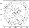Fig. 1 All stars (dots) and P-stars (asterisks) imaged near dwarf Nr.12 and the reference fields, shown by small (for R = 200 px) and large (for R = 1000 px) circles centered at the corresponding P-star.

4 Error terms in differential measurements and their calibration

For a target specified with P_i = 0, the observed variance ⟨Δ²⟩ of the residuals Δ is modeled by Eq. (1), but for a subset of reference P-stars with P_i > 0, a valid expression is ${\sigma }_{\text{mod}}^2=$ ${\sigma }_{\mathrm{p}}^2+{\sigma }_{\mathrm{a}}^2-{\sigma }_{\mathrm{r}}^2$ (Paper I). For consistency, we united them into a single expression: $${\sigma }_{\mathrm{m}\mathrm{o}\mathrm{d}}^2={\sigma }_{\mathrm{p}}^2\pm {\sigma }_{\mathrm{r}}^2+{\sigma }_{\mathrm{a}}^2,$$(5)

where ${\sigma }_{\mathrm{r}}^2$ is either added for the primary star or subtracted for the reference star. We omitted the term σ_extr since it was found to be small; thus, we expected that the observed variance ⟨Δ²⟩ would be approximately equal to ${\sigma }_{\text{mod}}^2$. Furthermore, we admitted a simple approximate relation, $${\sigma }_{\mathrm{r},(P_i>0)}^{-2}={\sigma }_{\mathrm{r},(P_i=0)}^{-2}+{({\sigma }_{\mathrm{p}}^2+{\sigma }_{\mathrm{a}}^2)}^{-1},$$(6)

between the reference frame noise in the above two cases (Paper I). In the next paragraphs, we specify expressions for these components used to find the initial estimates of σ_mod, and they are later updated in Sect. A.2.

The component σ_p in Eq. (5) is usually a dominant error component for even the brightest stars, and it is related to the statistical fluctuations of the photon number in pixels of the star image. For bright images and a low background noise, it depends on the full width half maximum (FWHM) and the full electron flux I_full in the star image. The theoretical expression ${\sigma }_{\mathrm{p}}=FWHM/\left(2.35\sqrt{I_{\text{full}}}\right)$ is given, for example, by Irwin (1985), Mendez et al. (2013) for Gaussian star image shape. For FORS2, the Gaussian approximation is not sufficient; thus, we represented the star profiles by a sum of three Gaussians where the core image component with a sigma parameter σ_G contains a flux I_G approximately equal to two-thirds of the total signal I_full (Paper I). Two other Gaussians represent the star profile widening in wings. For this compound model, the above-cited expression for σ_p is not valid, and a better empiric expression is $${\sigma }_{\mathrm{p}}=c_{1}FWHM/\left(2.34\sqrt{I_G}\right),$$(7)

where FWHM = 3.10σ_G (near 2.35σ_G, as expected for a Gaussian star profile) and c₁ = 1 + 0.15(σ_G − 1.5)² with σ_G expressed in pixels. This is a simplified expression valid for bright stars, and a full form is given in Paper I. All numeric terms in Eq. (7) of course slightly depend on seeing and varying geometry of star images. Equation (7) is therefore hardly expected to provide an exact estimate of ${\sigma }_{\mathrm{p}}^2$ for any image over a wide 0.5–1.0″ range of the seeing, which is a reason for the few percent of inconsistency between ⟨Δ²⟩ and ${\sigma }_{\text{mod}}^2$. By applying an extra scale-type calibration (Sect. A.2) of σ₂² (which can refer to numeric terms in expressions for FWHM and c₁), we arrived at a sufficiently good match of the model and the measured variances.

The reference frame noise ${\sigma }_{\mathrm{r}}^2$ for a star i, reference or primary, is defined by Eq. (4). It is accurate to within a few percent due to the above-discussed uncertainty in σ_p because it affects elements of the matrix F⁻¹.

As the initial raw model of ${\sigma }_{\mathrm{a}}^2$, we used the empirical expression $${\sigma }_{\mathrm{a}}^2=a(17/T)R^b$$(8)

valid for zenith (Lazorenko 2006). Here, the values of a and b are given in Table 1 of that paper for each reduction mode k. To be applicable in a general case, term a was preliminarily multiplied by a factor (sec z)^ν+p+1 (Sect. 5). Because the value of b is between 2.2 and 3.8, the ${\sigma }_{\mathrm{a}}^2$ variance quickly increases with R.

As commented, the above expressions are approximate only. Therefore, in Sect. A.2 we update them (individually for each P-star) by means of a calibration based on cross-comparison of the model to the measured variance ⟨Δ²⟩. Thus, ${\sigma }_{\mathrm{p}}^2,{\sigma }_{\mathrm{r}}^2$, and ${\sigma }_{\mathrm{a}}^2$ were updated as explained in Sect. A.2, and the following analysis was done with these nominal variances.

It is useful to compare the typical values of the terms in the budget of the total noise Eq. (5) for our P-stars. At an average seeing of 0.6″ and 0.1–0.5×10⁶ number of electrons in images, σ_p is 0.5–1.2 mas. The other two term magnitudes are between 0.1 and 0.5 mas or below, depending on the field star distribution, β, exposure, z, and R. Thus, the uncertainty of the photocenter measurement dominates, except short exposures, low k and wide R when σ_a increases. Also, at narrow R and high k the term σ_r may dominate because of the dependence σ_r ~ kR⁻¹ (Lazorenko & Lazorenko 2004).

5 Model of differential image motion

Image motion detected as a random displacement of star photocenter positions is caused by atmospheric turbulence, which introduces light phase fluctuations across the telescope entrance pupil and thus displaces differently the target object and reference star positions. A single layer turbulence concentrated at the altitude h works as the phase screen, which causes differential displacements in astrometric measurements. This random process is characterized by the 2D spectral power density (Lazorenko & Lazorenko 2004) $$G(q)=\frac{0.033(2\pi {)}^{1-p}{C}_n^2}{VT}Y(q)Q(q)q^{-2-p}\mathrm{\Delta }h,$$(9)

where q is a circular spatial frequency related to the screen, $C_n^2$ is the turbulent strength index in this layer, V is the wind velocity at the screen location, Δh is the layer thickness, and p is a constant, which in the case of the Kolmogorov turbulence is p = 2/3. Because there is some evidence of non-Kolmogorov-type turbulence (Lazorenko 2002), we treat the term p as a variable until in Sect. 6.4 we find that actually the observed data are fit well with p = 2/3, which is expected for Kolmogorov turbulence. Equation (9) is valid for long exposures T ≫ D/V and expresses the process of filtration of the light phase fluctuations by two filters specific to the measurements of differential displacements. The filter Y(q) = [2J₁(πDq)/(πDq)]² describes averaging of the phase fluctuations across a circular telescope entrance pupil D, and the filter Q(q) represents absorption of the DIM power spectrum by the grid of reference stars in differential astrometric measurements.

While Y(q) effectively reduces the high-frequency DIM spectrum, filter Q(q), $$Q(q)=N^{-2}\sum _{i,i^{\mathrm{\prime }}=1}^N{a}_i{a}_{i^i}[1-2J_0\left(2\pi dq{\rho }_i\right)+J_0\left(2\pi dq{\rho }_{i,i^{\mathrm{\prime }}}\right)],$$(10)

suppresses low-frequency components and represents absorption of the DIM power spectrum by a grid of i = 1, 2 . . . N reference stars imaged in the field of the angular radius R. Here, J₀ is a Bessel function of the first kind, ρ_i and ρ_i,i′ are the angular distance between the target i = 0 and the reference star i′ or between i and i′ reference stars, d = h sec z is the inclined distance to the turbulent layer for observations made at the zenith distance z, and a_i represents values that depend on the astrometric reduction mode k and are specified in Sect. 5.1.

The integration of function G(q) produces the variance of DIM $${\sigma }_{\mathrm{a}}^2=CI(d)\left(T_0/T\right)\sec z$$(11)

generated by a single turbulent screen where term $$C=0.033(2\pi {)}^{2-p}{C}_n^2{\left(V{T}_0\right)}^{-1}\mathrm{\Delta }h$$(12)

depends only on the atmospheric turbulence and is numerically equal to ${\sigma }_{\mathrm{a}}^2$ at exposure T₀ for observations characterized by a unit integral I. The integral $$I(d)={\int }_0^{\mathrm{\infty }}Y(q)Q(q)q^{-1-p}dq$$(13)

is a natural metric of DIM variance in a sense that ${\sigma }_{\mathrm{a}}^2$ depends on a numeric value of I that inherits most of the principal parameters of the observations: telescope aperture D, the current exposure specification (R, sec z), the star distribution in the field, photon flux from stars, background, and the inclined distance d = h sec z to the phase screen. Also, in Eq. (11), we added a factor sec z to take into account the additional increase of the turbulence proportionally to the depth of the turbulent medium for observations at zenith angle z. Modification of Eq. (13) for the von Karman spectrum (finite outer scale of turbulence) is considered in Appendix C.

The variance ${\sigma }_{\mathrm{a}}^2$ can be reduced for very narrow angle observations when Rd ≪ D/2, making the product of filters Y(q) and Q(q) small. In practice, it forces use of very large ground-based telescopes of the VLT class or bigger to ensure good precision with R ~1–2′. For narrow angle observations, the integral I(d) in Eq. (13) permits approximate dependence, $$I(d)\sim (Rd{)}^{\nu +p}{D}^{-\nu },$$(14)

on R, where ν is a constant related to the entrance pupil shape and which for a circular objective is ν = 3. Hence, according to Eqs. (11)–(13), the DIM variance ${\sigma }_{\mathrm{a}}^2$ generated by a single turbulent screen follows the dependence $${\sigma }_{\mathrm{a}}^2\sim C(Rh{)}^{\nu +p}{D}^{-\nu }(\sec z{)}^{\nu +p+1}\left(T_0/T\right).$$(15)

5.1 Modal structure of the image motion

Bessel functions in Eq. (10) can be expanded into an infinite series of even powers of q. Hence, Q(q) has a modal structure $Q(q)=\sum _{s=1}^{\mathrm{\infty }}{g}_{2s}{q}^{2s}$ with coefficients g_2s dependent on coordinates x_i, y_i of reference stars and the target object x₀, y₀ (Lazorenko & Lazorenko 2004; Lazorenko et al. 2014). The expressions for coefficients g₂,g_4··g_k−2 until some even integer mode $$k=2(\beta +1)$$(16)

can be represented (Paper I) as the sum of quadratic terms of the type ${[\sum _{i=1}^N{a}_i{f}_{iw}-f_{0,w}]}^2$.

Remarkably, all the terms g₂, ... up to and including g_k−2 can be turned to zero by a proper choice of coefficients a_i that meet w = 1,... k(k + 2)/8 conditions $\sum _{i=1}^N{a}_i{f}_{iw}-f_{0,w}=0$. One may note that the least-squares transformation (Sect. 3) to the reference frame (Eq. (2)) is made with a projection matrix a whose first-line elements meet the above conditions; at the same time, they are used in Eq. (10). Thus, the least-squares transformation leads to a complete elimination of low expansion modes 2s = 2,4... k − 2 of Q(q), which is now nearly opaque for frequencies below about q₀ = k/(4πRd) (Lazorenko & Lazorenko 2004). The result is a cutoff of the G(q) spectrum at low frequencies, which contains the principal energy of the DIM and consequently leads to a strong decrease of the integral (13) and σ_a values. An even integer k, referred hereto as the reduction mode, is the first active (not eliminated) mode of filter Q(q) with dominating energy, so that Q(q) ≈ g_kq^k. The effect of the image motion filtration favors use of the high k (or β) modes because it expands the opaque zone of filter Q(q).

It makes clear that it is not correct to speak of the DIM variance ${\sigma }_{\mathrm{a}}^2$ in general as the quantity dependent on the atmosphere only. Instead, we should specify the mode k of the transformation procedure and refer to the DIM variance as a function ${\sigma }_{\mathrm{a}}^2(k)$. Thus, the variance ${\sigma }_{\mathrm{a}}^2$ for the reduction with mode k = 6 is the measure of the DIM spectrum G(q) including the filter Q(q) modes q⁶, q⁸..., while the reduction with k = 8 is sensitive to modes q⁸, q¹⁰... With each subsequent k, we access different spectral ranges, with a natural decrease of ${\sigma }_{\mathrm{a}}^2$ at each next k value. Because the Q(q) filter suppresses frequencies below q₀, we find that the largest linear size of the phase fluctuations related to Q(q) is $$L_Q\simeq 4\pi Rd/k.$$(17)

For instance, at a distance of d = 18 km to the turbulent layer, a field size R = 2.1′, and k = 6, its value is L_q ⋍ 20 m irrespective of D. In particular, this means that the DIM is only marginally affected by the actual value of the outer scale of turbulence if it is longer than 20 m for telescopes of VLT or ELT size (Appendix C).

5.2 Metric integral I and its properties

The measured DIM variances (estimates of ${\sigma }_{\mathrm{a}}^2$) are not homogeneous and not directly comparable between fields because they correspond to different z. Of course, it is easy to reduce ${\sigma }_{\mathrm{a}}^2$ to zenith using the approximate dependence ${\sigma }_{\mathrm{a}}^2\sim (\sec z{)}^{\nu +p+1}$ of DIM variance on z valid for narrow fields Eq. (15), but it is possible to apply exact conversion, leading to a better accuracy. Another problem arises when we want to develop a universal model for ${\sigma }_{\mathrm{a}}^2$ that allows us to predict its value for any star field and for any altitude of the telescope above the sea level. In this case, we should take into consideration the fact that the ${\sigma }_{\mathrm{a}}^2$ value depends on the distribution of the stars. Moreover, they are not comparable even for P-stars within the same field because of essentially different values of I defined by Eq. (13). All of these problems are solved with the introduction of a standard star distribution. As this standard template, we considered easily handled continuous distribution of reference stars (CSD). The properties of I for the standard distribution allowed us to model ${\sigma }_{\mathrm{a}}^2$ based on the atmosphere turbulence data (Sec. 5.3) with a subsequent comparison to FORS2 observations.

5.2.1 Continuous distribution of reference stars

The value of ${\sigma }_{\mathrm{a}}^2$ is a linear function Eq. (11) of the metric I(d), which via the filter Q(q) significantly depends on the star distribution in the field and the brightness of the stars, and therefore, it is strongly variable. Its properties are easily analyzed in the tutorial case of continuous (non-discrete) distributions of equally bright stars completely filling the circular reference field and placing the target object exactly in the field center. These distributions serve as a good model of the FORS2 field’s properties, which in this study are located near the Galactic plane and are very rich in stars. We consider them to be a template distribution with expressions for Q(q) available as functions (Lazorenko & Lazorenko 2004) $$\begin{array}{rl}& \begin{array}{lll}& {[1+\frac{4J_1(y)}{y}-\frac{24J_2(y)}{y^2}]}^2,& k=6,8;\beta =2,3\\ Q(q)==& {[1-\frac{6J_1(y)}{y}+\frac{96J_2(y)}{y^2}-\frac{480J_3(y)}{y^3}]}^2,& k=10,12;\beta =4,5\\ & [1+\frac{8J_1(y)}{y}-\frac{240J_2(y)}{y^2}+\frac{2880J_3(y)}{y^3}& \\ & {-\frac{13440J_4(y)}{y^4}]}^2,& k=14,16;\beta =6,7\end{array}\end{array}$$(18)

of the variable y = 2πdqR, where dR is the linear size of a star field at distance d. Above, we added one more expression for k = 14, 16 derived using the analytic approach in Sect. 6.1 of the paper cited, where a factor (k/4 − i + 1)! in Eq. (41) is (due to a misprint) to be read as (k/4 + i − 1)!. For odd k/2 (for k = 6, 10, 14 or β = 2, 4, 6) functions, the value of Q(q) is identical to the nearby next even modes k/2 (for k = 8, 12, 16 or β = 3, 5, 7) because the least-squares solutions are identical in these cases at the target location (of course, solutions in other field points are different, but we note that function Q is defined for the field center only). Functions Q(q) in Eq. (18) are expanded into powers of spatial frequencies with the first non-zero member q^k, with all lower expansion terms turned to zero (Sect. 5.1). The integration Eq. (13) that uses expressions from Eq. (18) yields I_c(d, k, R) values for CSD as a function of d, R, and k, but in the following, we stick to a shorter designation I_c(d). Otherwise, we explicitly specify the variables.

Figure 2 makes a general impression on the absolute magnitude of I for CDS and for FORS2 fields for some parameters R and k. Both integrals approximately follow a power dependence R^ν+p; therefore, their change is over three decades within a quite moderate range of R.

At some fixed R, the values of I_c(d) increase quickly with d following a power law I_c(d,R) ~ d^ν+p (14) valid for narrow fields but not exactly. In order to examine minor deviations from the power law, we formed integrals $I_{\mathrm{c}}^{\ast }(d)=I_{\mathrm{c}}(d){\left(d_0/d\right)}^{\nu +p}$ normalized to some reference distance d₀ and computed at some fixed R. We adopted d₀ = 16 km because for this distance, we initially computed integrals I_F,i(d₀) for each i-th P-star in the FORS2 fields. For illustration, Fig. 3 presents normalized functions $I_{\mathrm{c}}^{\ast }(d)$ versus distance d to the phase screen. These functions vary quite moderately within a full range of distances, while the original function I_c change is ~ 1000.

We present $I_{\mathrm{c}}^{\ast }$ functions computed in two ways: one for a fully open circular entrance aperture of diameter D = 8.2 m and another for the actual VLT optical design with a secondary mirror of D_s = 0.9 m diameter. In the latter case, instead of Eq. (9), we used a modified expression Y(q) = [2J₁(πDq)/(πDq) − (D_s/D)²2J₁(πD_sq)/(πD_sq)]² derived from a difference of the Fourier transforms of two mirrors. The computed integrals in both cases are quite similar in shape, but in the following, we keep to the version with a secondary mirror.

The original metric integrals I_c and their modifications $I_{\mathrm{c}}^{\ast }$ in Fig. 3 were computed for even k/2 only because functions Q(q) and, consequently, the integrals for nearby smaller k are the same. For instance, the integral values for k = 6 and k = 8 are equal. Therefore, use of the higher k = 8 mode instead of k = 6 results in no decrease of $I_{\mathrm{c}}^{\ast }$, but the next k = 10 mode leads to a significant, roughly fivefold, decrease of $I_{\mathrm{c}}^{\ast }$ (and consequently of the DIM variance ${\sigma }_{\mathrm{a}}^2$).

We also note that Fig. 3 refers to R = 2.1′. For other R′, in accordance with the definition of the y variable in Eq. (18), the $I_{\mathrm{c}}^{\ast }(d)$ shape is the same if plotted versus a distance scaled with a factor R′/R.

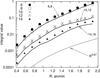Fig. 2 Metric integral I dependence on the field size R for CSD (thick solid lines) and for FORS2 fields in average (different symbols). Approximate dependence I ~ R3.67 (dashed line). All integral values were computed at d = 18 km.

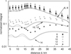Fig. 3 Normalized integral $I_{\mathrm{c}}^{\ast }(d)$ dependence on distance d to the turbulent phase screen for CSD if the VLT design is with (solid lines) or without a secondary mirror (dashed lines). Integral $⟨I_{\mathrm{F}}^{\ast }(d)⟩$ averaged over all P-stars (different type symbols for each k mode shown) within a sky field No. 12. Integral $I_{\mathrm{F},i}^{\ast }$ for each P-star in those fields (gray symbols, k = 6 only). Integrals were computed for R = 2.1′.

5.2.2 Metric Integral I for FORS2 fields

The integral I values for the FORS2 fields are easily evaluated in terms of effective reference field size S = ${\left|N^{-2}\sum _{i{i}^{\prime }}^N{a}_i{a}_i^{\prime }{d}^k({\rho }_i^k+{\rho }_{i^{\prime }}^k-{\rho }_{i{i}^{\prime }}^k)\right|}^{1/k}$; however, these estimates are approximate only (Lazorenko & Lazorenko 2004). In this study, we wanted to meet the best accuracy provided by diverse observational statistics. Therefore, we computed I values by direct integration. The numerical results were found to be quite stable to seeing conditions, and therefore, the computations were done using a single typical image in a sky field. We revealed quite similar features of this integral dependence on d for FORS2 and for CSD. This is illustrated, for example, in the field Nos. 12 and 14, for which we computed k_F,i for each calibration star i. For these fields, the normalized functions $I_{\mathrm{F},i}^{\ast }(d)=I_{\mathrm{F},i}(d){\left(d_0/d\right)}^{\nu +p}$ are quite similar in shape to the functions $I_{\mathrm{c}}^{\ast }(d)$ of the corresponding order k, but they differ a little in magnitude (Fig. 3). A useful quantity specifying this feature is the ratio $${\mu }_i=I_{\mathrm{F},i}^{\ast }(d)/I_{\mathrm{c}}^{\ast }(d)=I_{\mathrm{F},i}(d)/I_{\mathrm{c}}(d)$$(19)

formed for each i-th calibration star. We find that it nearly does not depend on d, so we could assume that μ_i = const within a sky field for each i at a fixed k and R. At the same time, in different fields, its magnitude can vary between 0.5 and 1.5, with a scatter more often detected for k/2 odd (k = 6, 10, 12). Especially distinct variability is detected at smaller R ≈ 0.5′. Even in a single field variation of μ_i for the nearby calibration stars are quite significant (compare the scatter of individual I_F,i marked by gray symbols in Fig. 3) but natural and caused by use or exclusion of only a single bright (nearby calibration) star in the list of reference stars. A stronger concentration of bright stars in the field center leads to smaller I_F,i values and the least amount of scatter of their individual values.

The significant variability of I_F,i in star fields should be taken into consideration in this study in cases (Sect. 6.4) where we want to derive image motion characteristics for a typical (average) FORS2 field. Therefore, to remove the variable component in μ_i dependent on the sample, we averaged these values over calibration stars and star fields and obtained the terms ⟨μ_k,R⟩ or typical excesses of I_F,i over I_c at fixed k and R, shown in Fig. 4 as a function of R. We note that we found a small value for the excess of μ over a unit for even k/2, which indicates a good astro-metric quality of reference fields near the Galactic plane. For odd k/2, the discreteness of the star distributions led to a large, about 30%, excess at R = 2.1′. For narrower fields, this effect increases further to ~50%. Thus, for odd k/2, use of the next k + 2 reduction mode decreases the variance ${\sigma }_{\mathrm{a}}^2$ by the values indicated.

Some useful expressions for the computation of the FORS2 metric integral at any d and R are given in Appendix B. In the following analysis, we often refer to these expressions.

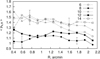Fig. 4 Average excesses ⟨μk,R⟩ of integrals IF for FORS2 over Ic for CSD, for each reduction mode k (different symbols). Approximate 1-sigma uncertainty of ⟨μk,R⟩ due to variations of μk,R in separate sky fields (error bars).

5.3 Model of the DIM variance based on the turbulence profile

As commented in this section, a single atmospheric turbulent layer causes the DIM variance ${\sigma }_{\mathrm{a}}^2$ expressed by Eq. (11). A full cumulative atmosphere effect in the zenith is a sum over all layers $${\sigma }_{\mathrm{a}}^2=\left(T_0/T\right)\sum _j{C}_{j}I\left(h_j\right),$$(20)

where h_j is the layer altitude above the telescope (2.65 km above the sea level) and C_j (defined by Eq. (12)) is its input to the DIM variance at exposure T = T₀ and I(h_j) = 1. The impact of the layers strongly depends on h_j because $I\left(h_j\right)\sim h_j^{\nu +p}$, in accordance with Eq. (15). This is illustrated by Fig. 5, where $C_n^2$ is the median turbulent index for the VLT site, which we adopted as a combination of observed data (Osborn et al. 2018; Sarazin et al. 2017; Butterley et al. 2020), and the wind velocity provided by radio soundings (Masciadri et al. 2013). The range of the effective altitudes is narrow and limited by 16–18 km only because the DIM is strongly suppressed at low altitudes by the factor h^ν+p peculiar to astrometric reduction procedure and, at higher h, by the decrease of $C_n^2$. Within this narrow range of h, approximation (B.2) is precise enough to estimate I(h_j) at any h_j via its value at some reference altitude 16 ≤ h_ref ≤ 18 km as I(h_j) = F(h_j)/F(h_ref)I(h_ref)(h_j/h_ref)^ν+p because a ratio F(h_j)/F(h_ref) is nearly a unit within this range of altitudes. We let h_ref = 18 km, and hence we arrived at a rough but useful approximation, $${\sigma }_0^2=A_{0}I\left(h_{\text{ref\hspace{0.17em}}}\right)\left(T_0/T\right),$$(21)

for ${\sigma }_{\mathrm{a}}^2$, where $$A_0={\tau }_0\sum _j{C}_j{\left(h_j/h_{\mathrm{r}\mathrm{e}\mathrm{f}}\right)}^{\nu +p}.$$(22)

The above expressions allowed us to easily find ${\sigma }_0^2$ by summation over turbulent layers, which is the estimate of ${\sigma }_{\mathrm{a}}^2$ at zenith. In view of the following results, we inserted a factor τ₀ = 0.84 just to make roughly equal the model and the DIM variances measured with FORS2. With the measured turbulence data adopted and shown in Fig. 5 and T₀ = 30 s, we found A₀ = 44.5 mpx² = 0.708 mas². It is equal to ${\sigma }_0^2$ in the case of an imaginary star field with a unit integral I(h_ref) and T = 30 s; thus, σ₀ = 0.841 mas. Half of the variance ${\sigma }_0^2$, or 22.3 mpx² = 0.35 mas², is generated at 16–18 km altitudes. For fields with an arbitrary star distribution, ${\sigma }_0^2$ is consequently computed with Eq. (21), which by its content coincides with Eq. (11) for a single layer at z = 0 but generalized to the full atmosphere; in addition, it contains the predicted amplitude A₀. The integral I(h_ref) depends on R and the reduction mode k and should be computed using Eq. (13) with the Q(q) function with the actual star distribution and the corresponding brightness at d = 18 km.

The estimate of A₀ refers to some average atmospheric conditions, but we note that instant turbulent profiles are strongly variable (Le Louarn et al. 2000, Fig. 2). For instance, the rms variability of $C_n^2$ and V per day mounts roughly to 50% of its average value (Masciadri et al. 2013); therefore, a similar uncertainty is expected in the DIM estimates based on Eq. (22). Some deviations between the sources of the turbulence profile measurements we used and a lack of precise data on V at high altitudes lead to a roughly 20% uncertainty in the prediction of ${\sigma }_{\mathrm{a}}^2$; therefore, we expect that our estimate of A₀ is accordingly approximately accurate. In particular, not having a unit value of τ₀ is probably due to an inconsistency between the adopted profile in Fig. 5 and the actual turbulent profiles, or, alternatively, due to the finite outer scale of turbulence (Appendix D). The actual variations of $C_n^2$ for a single night mount to an even larger ±50% relative uncertainty of the DIM.

The expressions (21)–(22) are applicable to any R and k, as they are universal in this respect, and they are easy to apply. However, they were obtained assuming the exact validity of the dependence I(h_j) = I(h_ref)(h_j/h_ref)^ν+p. More accurate estimates based on this model can be obtained using numeric values of integrals I_c(d) or I_F(d) expressed by Eq. (B.1) for summation over altitudes, which results in the variances $$\begin{array}{rl}& {\sigma }_{\mathrm{c}}^2(k,R)=\left(T_0/T\right){\sum }_j{C}_j{I}_{\mathrm{c}}(h_j,k,R)\\ & {\sigma }_{\mathrm{F},i}^2(k,R)=\left(T_0/T\right){\mu }_{i,k,R}{\sum }_j{C}_j{I}_{\mathrm{c}}(h_j,k,R)\end{array}$$(23)

representing estimates of ${\sigma }_{\mathrm{a}}^2$ for each R and k. Here, the second line refers to the DIM variance in FORS2 fields for an individual star i, and it contains the factor μ_i,k,RI_c(h_j, k, R) defined by Eq. (19) and which in the narrow range of effective altitudes is nearly independent on h_j. It is useful to rewrite Eq. (23) as $$\begin{array}{rl}& {\sigma }_{\mathrm{c}}^2(k,R)=A_{\mathrm{c}}(k)I_{\mathrm{c}}(h_{\mathrm{r}\mathrm{e}\mathrm{f}},k,R)\left(T_0/T\right)\\ & {\sigma }_{\mathrm{F},i}^2(k,R)=A_{\mathrm{c}}(k)I_{\mathrm{F},i}(h_{\mathrm{r}\mathrm{e}\mathrm{f}},k,R)\left(T_0/T\right),\end{array}$$(24)

keeping a linear dependence of the variance on I_c(h_ref) or I_F,i(h_ref) (computed at a given k and R) just as in the approximate model (21), but instead of A₀, there are a better defined terms $$A_{\mathrm{c}}(k)=\sum _j{C}_j{I}_{\mathrm{c}}(h_j,k,R)/I_{\mathrm{c}}(h_{\mathrm{r}\mathrm{e}\mathrm{f}},k,R)$$(25)

that are functions of k and R and universally defined both for the CSD and FORS2 fields. We computed A_c(k) for each R and found that the variation of these terms with R is within ±10%, and it can therefore be neglected. Thus, in Table 2 we give their median over R as an adequate approximation. Also, because the variation of values A_c(k) with k is moderately low, we find that sometimes it is reasonable to represent them roughly with a single quantity A_c(⟨k⟩) = 0.701 mas² (or σ_c = 0.837 mas) that is the weighted average over k. We conclude that Eq. (24), which is the updated version of the model (21), leads to the estimate close to the amplitude A₀ = 0.708 mas² obtained for a simpler model based on approximation of the very narrow fields.

Furthermore, we found that the variances ${\sigma }_{\mathrm{c}}^2$ and ${\sigma }_{\mathrm{F}}^2$ computed with Eq. (23) are numerically well fit by a power dependence $$\begin{array}{rl}{\hat{\sigma }}_{\mathrm{c}}^2(k,R)& =a_{\mathrm{c}}^2(k)F_{\mathrm{e}\mathrm{f}\mathrm{f}}^2(R){\left(R/R_0\right)}^{\nu +p}\left(T_0/T\right)\\ {\hat{\sigma }}_{\mathrm{F}}^2(k,R)& =a_{\mathrm{F}}^2(k)F_{\mathrm{e}\mathrm{f}\mathrm{f}}^2(R){\left(R/R_0\right)}^{\nu +p}\left(T_0/T\right)\end{array}$$(26)

on the field size R. This representation follows from Eq. (B.4), and $F_{\text{eff}}^2(R)$ is the effective value of the function F(d₀R/R₀) accumulated over all layers. The fit terms $a_{\mathrm{F}}^2(k)$ we computed in approximation $F_{\text{eff}}^2(R)=1$ and by replacing I_F,i(h_ref) in Eq. (24) by ⟨μ_k,R⟩I_c(h_ref) therefore ${\sigma }_{\mathrm{F}}^2(k,R)$ refer to typical FORS2 fields. The amplitude terms computed for R₀ = 1′ and T = T₀ are given in Table 2. We find that $a_{\mathrm{F}}^2(k)>a_{\mathrm{c}}^2(k)$ mostly for k = 6, 10, 14, which is in accordance with the excess in function ⟨μ⟩ values demonstrated by Fig. 4.

We summarize this section with a remark that the ${\sigma }_{\mathrm{a}}^2$ can be modeled either by direct summing Eq. (B.4) over each layer input to the DIM variance or alternatively by compressing all the turbulence into a single layer at h_ref, with an amplitude Eq. (25) caused by all the atmosphere (Eq. (24)). In the following, we compare the derived estimates based on the turbulence profile and on the actual observations.

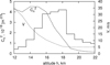Fig. 5 Relative input to the DIM variance (steps) induced by turbulent layers with the measured turbulent index $C_n^2$ (dashed) and the wind velocity V (dotted). Altitude h is above the VLT telescope.

6 DIM variance derived from FORS2 observations

According to Eqs. (21) and (24), we expected that the DIM variance for FORS2 observations, in zenith, to be proportional to I(h_ref). This is valid if our concept of the DIM effect (Sect. 5) is correct and, on the other side, astrometric reduction of FORS2 observations and extraction of the DIM variance were performed sufficiently good. This was a key item of investigation to verify in the next Sections.

6.1 Conversion to zenith

At first, we reduced the observed variances ${\sigma }_{\mathrm{a}}^2$, which refer to some zenith angle z, to zenith. As discussed in Sec. 5.3, the effective range of the altitude of the turbulent layers is very narrow, from 16 to 18 km. For this reason, we could assume that the DIM effect from a full atmospheric depth is approximately equal to that from a single layer located at some reference altitude h_ref within this range. Then, according to Eq. (11), the measured DIM variance is proportional to I(h_ref sec z). Using conversion (B.2) of the integral from the inclined distance h_ref sec z to h_ref, we found that the measured estimate of ${\sigma }_{\mathrm{a}}^2$ at zenith is $${{\sigma }_{\mathbf{a}}^2|}_{z=0}(k,R)={{\sigma }_{\mathbf{a}}^2|}_{z>0}[F\left(h_{\text{ref\hspace{0.17em}}}/F(h_{\text{ref\hspace{0.17em}}}\sec z)\right](\sec z{)}^{-\nu -p-1}.$$(27)

In this way, we transformed the observed variances to conditions comparable for all fields, thus arriving at a uniform dataset to be analyzed jointly. Conversion (27) is quite stable in respect to h_ref choice because the ratio F(h_ref /F(h_ref sec z) is not very sensitive to this term value. Further reduction to the standard exposure T₀ = 30 s provided variances $${\sigma }_{\mathrm{a}}^2(k,R)={{\sigma }_{\mathrm{a}}^2|}_{z=0}\left(T/T_0\right),$$(28)

that are also not dependent on T.

6.2 Dependence of FORS2 DIM variance on the integral I

Considering that the location of the effective turbulence is likely within 16 and 20 km, reduction to zenith was made for a sequence of reference altitudes h_ref in this range, with the results, in terms of ${\hat{\sigma }}_{\mathrm{F},i}^2$, deviating within ±2% only. In parallel, we converted I_F,i(d₀), computed originally for d₀ = 16 km, to this set of distances d = h_ref using Eq. (B.2). In this way we converted both the observed DIM variances and the integrals I_{F, i} to conditions uniform for all fields irrespective of z and T.

We proceeded with validation of the approximate model Eq. (21), assuming that ${\sigma }_0^2$ and I(h_ref) in this equation are represented, respectively, by a set of the measured values ${\sigma }_{\mathrm{a},i}^2(k,R)$ and I_F,i(h_ref, k, R) for each i-th P-star irrespective of its status (primary or reference). Thus, we wanted to find whether ${\sigma }_{\mathrm{a},i}^2(k,R)$ is a linear function of I_F,i(h_ref) not taking dependence on the k mode into consideration. The immediate fit of these data with Eq. (21), however, revealed a certain systematic pattern in the fit residuals at small R ≤ 1′ very similar in all sky fields for each separate k. We found that this inconsistency is well modeled by two offset terms, off_k and ${\delta }_k^{\ast }$, that are introduced for each k. The first term is a general offset to the DIM variance, and the second is a correction to the zero-point of the adopted reference frame uncertainty (parameter δ_r in Eq. (A.4)). These terms were incorporated for each k mode separately, and instead of Eq. (21), we used the updated model of DIM variance, $${\sigma }_{\mathrm{a},i}^2(k,R)={\hat{A}}_0{I}_{\mathrm{F},i}\left(h_{\mathrm{r}\mathrm{e}\mathrm{f}}\right)+{\mathrm{o}\mathrm{f}\mathrm{f}}_k+{\delta }_k^{\ast }{R}_i^{-2},$$(29)

to fit the full set of measurements combined for all P-stars, k, and R. Here, ${\delta }_k^{\ast }{R}_i^{-2}$ is a minor approximate correction to ${\sigma }_{\mathrm{r},i}^2$. Both offsets produce an effect below ±0.005 mas² (= ±0.3 mpx²), or about 2–4% of the DIM variance magnitude in the range of R from 0.7 to 2.1′, which is the most important for this variance derivation. We repeated computations with different h_ref, and they led to quite a similar quality of the fit, but with a slightly better convergence of the residuals for h_ref = 18 km. Therefore, in the following we used this parameter value as the best, and the I_F,i values refer to this distance from hereon.

Figure 6 demonstrates the good linearity of the measured variances ${\sigma }_{\mathrm{a},i}^2(k,R)$ on I_F for a full data set using all k modes. We derived Â₀ = 0.715 mas² = 44.95 mpx² with a formal uncertainty of ±0.002 mas² = ±0.13 mpx². This is close, but it is a factor 1.009 over the A₀ or a factor τ = 1.019 over the A_c(⟨k⟩) (averaged over k) estimates expected from the model Eq. (21). In the following, we recomputed the variances ${\sigma }_{\mathrm{a},i}^2(k,R)$, applying corrections for the offset terms off_k and ${\delta }_k^{\ast }{R}_i^{-2}$.

We proceeded in this investigation as described above but separately for each k reduction mode. We wanted to fit the measured variances ${\sigma }_{\mathrm{a},i}^2(k,R)$ with a linear function, $${\sigma }_{\mathrm{a},i}^2(k,R)=A_{\mathrm{F}}(k)I_{\mathrm{F},i}(h_{\mathrm{r}\mathrm{e}\mathrm{f}},k,R),$$(30)

similar to Eq. (29) using data for each mode k separately. The derived values (Table 3) slightly deviate from Â₀, and the deviation pattern correlates well with A_c(k) in Table 2. We show this in Fig. 7, where A_F(k) is compared with τA_c(k) using a factor τ = 1.019 applied to match the model to FORS2 estimates at k averaged. For most k, the inconsistency between both estimates is within three sigma, meaning that the extraction of the DIM variance from FORS2 astrometry is correct, and the conservative accuracy of the coefficients A_F(k) derivation is better than 2% when considering the worst mismatch between τA_c(k) and A_F(k). These conclusions also remain valid for von Karman turbulence (Appendix D).

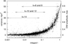Fig. 6 Measured variance ${\sigma }_{\mathrm{a},i}^2(k,R)$ at zenith for the 30 s exposure as a function of IF metric computed at href =18 km for all k modes mixed and a full data set (dot sizes show the star brightness). A linear Eq. (29) fit (solid line) visually coincides with the model dependence (21) based on the turbulence profile. Typical ranges of IF for each k are shown.

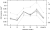Fig. 7 DIM variances AF(k) (solid) and ĀF(k) (dashed lines) derived from FORS2 astrometry at any seeing for each k (and k modes mixed); the variances τAc(k) derived from the model Eq. (24) at τ = 1.019 are shown by circles. Average of AF(k) and ĀF(k) for a good 0.4–0.6″ and worse 0.8–1.0″ seeing are shown by dash-dotted and dotted lines, respectively. The right axis τ is the ratio of DIM variances to A0 = 0.708 mas2 estimated with the model Eq. (21).

6.3 Direct comparison of the observed and atmospheric turbulence model variances

We exploited another yet slightly different possibility in order to directly compare the measured ${\sigma }_{\mathrm{a},i}^2(k,R)$ variances for each P-star to those expected from the turbulence model. For that purpose, we computed the DIM variance at zenith for the adopted atmospheric model for each P-star, which in accordance with Eq. (24) is ${\sigma }_{\mathrm{F},i}^2(k,R)={\mu }_{i,k,R}{\sigma }_{\mathrm{c}}^2(k,R)$ at T = T₀, and using terms μ_i,k,R individually for each star. Then we assumed that the observed ${\sigma }_{\mathrm{a},i}^2(k,R)$ and the model ${\sigma }_{\mathrm{F},i}^2(k,R)$ variances are equal with an accuracy to the scaling fit parameter $\overline{\tau }(k)$: $${\sigma }_{\mathrm{a},i}^2(k,R)=\overline{\tau }(k){\sigma }_{\mathrm{F},i}^2(k,R).$$(31)

Thus, the corrected estimate of the DIM amplitude in Eq. (25), which now matches the FORS2 observations for each k separately, is $${\overline{A}}_{\mathrm{F}}(k)=\overline{\tau }(k)A_{\mathrm{c}}(k).$$(32)

The fit parameters $\overline{\tau }(k)$ and the corresponding DIM amplitudes Ā_F(k) computed with Eq. (32) are given in Table 3. The amplitudes match well with the A_F(k) derived also from FORS2 data (Fig. 7) but differ over three sigma from the τ(k)A_c(k) correspondent to the turbulence model. We consider that the possible reason of this discrepancy is a minor variability of μ_i,k,R with d, which we neglected in the computation of both values, and of course the inconsistency between the actual and the model turbulence. In any case, the relative discrepancy is below about 3% and is thus sufficient for practical purposes.

Figure 8 compares the observed ${\sigma }_{\mathrm{a},i}^2(k,R)$ with the model ${\sigma }_{\mathrm{F},i}^2(k,R)$ variances for all k modes. It also shows a linear dependence (31) with the parameter $\overline{\tau }(⟨k⟩)=1.002\pm 0.002$ equal to the average of $\overline{\tau }(k)$ overall k. This parameter value is comparable at five sigma to the ratio τ = 1.019 ± 0.002 between FORS2 and the model data obtained as described above in this Section. Furthermore, with Eq. (32), we derived Ā_F(⟨k⟩) = 0.703 ± 0.002 mas² (= 44.2 mpx²) near the parameter A₀ value defined by Eq. (22).

Considering that the coefficients A_F(k) and Ā_F(k) in Table 3 are little dependent on k, we found a quite accurate approximation, $${\sigma }_{\mathrm{a}}\approx (860\pm 40)\mu \mathrm{a}\mathrm{s}\sqrt{I(k,R)}{\left(T_0/T\right)}^{0.5},$$(33)

valid for polynomial orders β from two to six. Here, T₀ = 30 s and the metric integral I(k, R) is computed at h_ref = 18 km. This equation allows one to roughly estimate σ_a without any computations of the integral I, instead taking its approximate value from Fig. 2.

As an additional control, we inspected the sample of the least-squares fit of Eq. (29) residuals. If the data treatment is correct, they should have a Gaussian distribution with a sigma parameter: $$\epsilon =E{\hat{\sigma }}_{\mathrm{m}\mathrm{o}\mathrm{d}}^2\left[F\left(h_{\mathrm{r}\mathrm{e}\mathrm{f}}\right)/F(h_{\mathrm{r}\mathrm{e}\mathrm{f}}\sec z)\right](\sec z{)}^{-\nu -p-1}\left(T/T_0\right),$$(34)

where the E values are those already derived in Sect. A.2.1 for each field and are of the order of a unit. We find that after normalization with ϵ, they are distributed approximately by a normal law, with a moderate asymmetry in the histogram of the residuals. Further, the rms of the normalized residuals is equal to 1.03, near the expected unit value.

We also tested the stability of the A_F and Ā_F terms with seeing by splitting data into a few narrow FWHM ranges, and we found a moderate increase of the DIM variance by about 20% when comparing the best seeing (FWHM = 0.4–0.6″) to the worst (0.8–1.0″) seeing (Fig. 7). Thus, they are comparable in spite of a twofold seeing variation. Hypothetically, this increase can be caused by a weak correlation between the FWHM and the $C_n^2$ at high altitudes, which leads to the observed effect. Some evidence of an actual correlation between these quantities has been found by Sarazin et al. (2017), who formed average $C_n^2$ profiles over Paranal for different classes of atmospheric conditions, particularly when the turbulence concentrated above the ground layer is high or when it is low along any altitudes. The value of $C_n^2$ in the first case is a factor of three over that in the second case (Sarazin et al. 2017, Fig. 9) for altitudes 5–13 km. This is also reflected in a nearly twofold-different median seeing, correspondingly 0.76″ and 0.46″, which is quite near the FWHM ranges we tested. We numerically verified that the 5–13 km altitudes produce about 8% of the DIM variance; thus, the twofold increase of $C_n^2$ at these altitudes is likely sufficient to explain the 20% change in the DIM variance considered. However, we also admit the possibility that the detected change of the DIM variance with seeing is false and caused by an insufficiently good reduction model. In this case, we should restrain ourselves to the results derived for the average seeing.

In this section, we have demonstrated that the measured DIM variance matches that expected for the turbulence profile over a wide (three decades) range of the metric integrals’ change and data represented by the mix of parameters R, k, for observations obtained under various star distributions in sky fields and variable seeing. We conclude the following:

• The astrometric reduction of the FORS2 observations, the calibration of error terms, and the extraction of the DIM variance were performed sufficiently well;

• The FORS2 data, treated with different approaches, produced estimates of the DIM amplitude in zenith in the range of 0.705–0.722 mas² for a 30 s exposure and a reference field with a unit integral I. This is 0.995–1.019 of the value based on the turbulent vertical profile if it was preliminary scaled by a factor τ₀ = 0.84;

• The DIM variance is stable to within ±20% of its variations with respect to the seeing change.

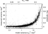Fig. 8 Same as in Fig. 6 but the horizontal axis refers to the DIM variance (24) based on the vertical turbulence profile and using I for each P-star. The fit function (31) with parameter $\overline{\tau }(⟨k⟩)$ is shown with a solid line.

6.4 Dependence of the DIM variance on the field size

The significant variability of the metric integral I_F,i between the individual P-stars and star fields is a problem when we consider the dependence of the measured ${\sigma }_{\mathrm{a},i}^2(k,R)$ on R or T. This is because ${\sigma }_{\mathrm{a},i}^2\sim I$ above the effect propagates to a significant scatter of individual DIM measurements at a fixed R or T, and it can be erroneously interpreted as incorrect data processing. Moreover, it can bias the model parameter estimates. Of course, this is of no importance for the modeled dependence of ${\sigma }_{\mathrm{a},i}^2(k,R)$ on I, whose variations are directly ingested by a linear function Eq. (29). In the following, we tried to reduce these problems.

As commented, because the ${\sigma }_{\mathrm{a},i}^2$ variances (28) are not exactly comparable in the domain of R, we converted them to normalized quantities (Fig. 9), $${\sigma }_{R,i}^2(k,R)=⟨{\mu }_{k,R}⟩{\sigma }_{\mathrm{a},i}^2(k,R)I_{\mathrm{c}}(h_{\mathrm{r}\mathrm{e}\mathrm{f}},k,R)/I_{\mathrm{F},i}(h_{\mathrm{r}\mathrm{e}\mathrm{f}},k,R),$$(35)

that are free from variations of values I_F,i(h_ref) for individual stars and rather represent the expectation of the DIM variance ${\sigma }_{\mathrm{a}}^2$ for a typical star field in the Galactic plane at a given R and k. Because in this study the data was split into 11 discrete sizes of R, within each R, we averaged the individual i-star estimates Eq. (35) to $⟨{\sigma }_{R,i}^2(k,R)⟩$, thus deriving well-defined estimates of the DIM variances ${\sigma }_{\mathrm{a}}^2$ shown in Fig. 9 by circles. At this step, we expected that individual estimates of ${\sigma }_{R,i}^2(k,R)$ are distributed as Gaussian values with a mathematical expectation $⟨{\sigma }_{R,i}^2(k,R)⟩$ and a sigma parameter ϵ₀(k,R) = ϵ⟨μ_k,R⟩I_c(h_ref, k,R)/I_F,i(h_ref, k, R), with ϵ defined by Eq. (34). We formed a histogram of normalized deviations ${\sigma }_{R,i}^2(k,R)-⟨{\sigma }_{R,i}^2(k,R)⟩$ for the data accumulated over R (each k mode was handled separately) and compared it with the normal law (Fig. 10). The observed distribution is slightly asymmetric, but it has a width parameter of approximately one unit (0.99 on average). We consider that this match with a normal distribution is sufficiently good, which suggests the level of correctness of the data processing.

To model the dependence of the observed variances ${\sigma }_{R,i}^2(k,R)$ on R, we fit them, for each k separately, by the expression $${\hat{\sigma }}_{R,i}^2(k,R)={\hat{a}}_R^2(k)F_{\mathrm{e}\mathrm{f}\mathrm{f}}^2(k,R){\left(R/R_0\right)}^{\nu +p}$$(36)

with a single free parameter â_R(k). By its structure, the function (36) is equivalent to Eq. (26), both representing the model fitting of the measured ${\sigma }_{R,i}^2(k,R)$ or the turbulence-based variances ${\sigma }_{\mathrm{F}}^2(k,R)$ via expressions valid for narrow fields. The terms ${\hat{a}}_R^2(k)$ are therefore the measured equivalent of the model amplitudes $a_{\mathrm{F}}^2(k)$ in (26). For computations, we assumed that $F_{\mathrm{eff}}^2(k,R)=$ 1 is a good approximation, which requires only some small second-order corrections applied later.

The amplitudes â_R(k) derived for each reduction k mode (with χ² = 1.07 reduced residuals of the fit) are given in Table 4 for exposure T = 30 s and R₀ = 1′. Computations were made for the data with any seeing and separately for good and bad seeing. We found an about 10% increase of the amplitude in the observations under bad seeing conditions, which agrees with a similar 20% increase of the DIM variances found in Sect. 6.3.

In addition, we modified the model Eq. (36), introducing an extra free fit parameter instead of the constant order ν + p = 3.67. We derived the estimates 3.73 ± 0.06, 3.75 ± 0.06, 3.39 ± 0.07, 3.74 ± 0.07, and 3.91 ± 0.31, listed in ascending order of k from six to 14, correspondingly. The average is 3.65, which actually coincides with the 3.67 expected for the Kolmogorov turbulence. The only over three-sigma deviation is seen for k = 10, probably due to a high (0.97) correlation between the model parameters â_R and ν + p. Thus, our data support the Kolmogorov type of the turbulence at altitudes 16–18 km.

Using the coefficients ${\hat{a}}_R^2(k)$ in Table 4 and Eq. (36), it is easy to find the DIM variance σ_a for any field size R. However, we should note a problem, namely that the coefficients ${\hat{a}}_R^2(k)$ in Eq. (36) were obtained with approximation of $F_{\text{eff}}^2(k,R)=$ 1 because these terms are unknown. In order to handle this problem, we exploited CSD as a good imitator of the FORS2 fields properties easily modeled for any R. This observation allowed us to note a similar problem for CDS fields when the variances ${\sigma }_{\mathrm{c}}^2(k,R)$ in Eq. (23) were fit by the model Eq. (26) under the approximation $F_{\text{eff}}^2(k,R)=1$. In this case, the quantity ${\hat{F}}^2(k,R)={\sigma }_{\mathrm{c}}^2(k,R)/{\hat{\sigma }}_{\mathrm{c}}^2(k,R)$ applied as a correcting factor to ${\hat{\sigma }}_{\mathrm{c}}^2(k,R)$ in a trivial way removes the mismatch between the functions referred to here for the CSD fields, allowing one to restore ${\sigma }_{\mathrm{c}}^2(k,R)$ values via parameters $a_{\mathrm{c}}^2(k)$. Quite similarly, calibration of ${\hat{\sigma }}_R^2(k,R)$ with this factor removes the problem for FORS2 fields. Of course, the terms ${\hat{F}}^2(k,R)$ we estimated at R₀ are exactly equal in both fitting expressions (23) and (36), that is at R₀ = 1′. The computed values $\hat{F}(k,R)$ are all ±0.05 near to a unit, except for the smallest value R = 0.5′, where some deviations mount to ±0.13. It follows that use of Eq. (36), which does not contain a factor $F_{\text{eff}}^2$, is quite sufficient to derive the DIM variance with an accuracy to ~5%.

To find more accurate estimates of DIM amplitudes, we used $\hat{F}(k,R)$ as a scaling calibrator to (â_R(k) + â_T(k))/2 and computed σ_a for a few field sizes (Table 5). Due to the large quantity of statistics used, the formal uncertainty of these estimates is about 1% only. However, we note that for a single randomly selected sky field, even in the Galactic plane, we expect to encounter strong variations of μ_i,k, due to the peculiar distribution of the stars, leading to variations of the metric integral and DIM variance. Therefore, in Table 5 we give uncertainties that treat typical fluctuations of star distribution in fields expressed by μ_i,k as a random event. This is useful to predict a_R(k, R) by guessing for a randomly selected field near the Galactic plane without taking into consideration the details of star distribution. Numerically, this type of uncertainty exceeds the formal uncertainty very much, roughly by a factor of ten to 20. In many cases, it mounts to ~20% of the σ_a value, or even more.

Considering a decrease of â_R(k) for high k and low R, one can expect significant improvement of the astrometric accuracy when applying the extreme values of these parameters. However, its value, modeled by the quantity σ_mod in Eq. (1), is the sum of all noise components. Therefore, it is a bivariate function of k and R. The interplay between these variables is not obvious and depends on the peculiarity of the observations. In particular, while σ_r decreases with the increase of R, the component σ_a follows a reverse dependence. Hence, the minimum of σ_mod occurs at some optimal R size where σ_r = σ_a (Lazorenko 2006). For our observations, this value is usually between 0.5 and 1.5′, depending on k and the actual star distribution. A curious feature is that use of different sets of k and R often lead to a quite moderate (~20%) improvement in σ_mod.

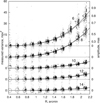Fig. 9 Each star variance ${\sigma }_{R,i}^2(k,R)$ as a function of field size R (dots; sizes are proportional to star brightness) for each reduction mode, their average $⟨{\sigma }_{R,i}^2(k,R)⟩$ for each R (large circles), fit functions Eq. (36) (solid), and the DIM variance ${\sigma }_{\mathrm{F}}^2(k,R)$ (Eq. (26)) based on the atmospheric model (dashed lines). For better visualization, the plots for each k > 6 are shown with a negative offset. The dots are dispersed horizontally for different star fields.

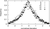Fig. 10 Frequency distribution of the normalized deviations ${\sigma }_{R,i}^2(k,R)-$ $⟨{\sigma }_{R,i}^2(k,R)⟩$ for a full sample of DIM probes at each reduction mode k (different signs). The normal distribution is shown with a solid line.

6.5 Dependence of the DIM variance on exposure

We tested also a well-known inverse dependence, Eq. (11), of ${\sigma }_{\mathrm{a}}^2$ on T for long exposures. For that purpose, we reduced the variances ${{\sigma }_{\mathrm{a},i}^2|}_{z=0}$ computed with Eq. (27) and related to zenith to the variances $${\sigma }_{T,i}^2(k)={⟨{\mu }_{k,R}⟩{\sigma }_{\mathrm{a},i}^2|}_{z=0}{I}_{\mathrm{c}}(h_{\mathrm{r}\mathrm{e}\mathrm{f}},R)/I_{\mathrm{F},i}(h_{\mathrm{r}\mathrm{e}\mathrm{f}},R){\left(R_0/R\right)}^{\nu +p}.$$(37)

In this way, due to a factor (R₀/R)^{ν +p}, the data obtained with several field radii R were converted to some common field size R₀. For verification, we used all the measurements available at R > 1.6′, where the DIM signal is highest, thus converting most of the accumulated data to conditions that differ by exposure T only. Values ${\sigma }_{T,i}^2$ obtained with R₀ = 1′ and that refer to a typical star field at the Galactic equator were fit by the model $${\sigma }_{T,i}^2(k)={\hat{a}}_T(k{)}^2{\left(T_0/T\right)}^{B(k)}$$(38)

with two free parameters â_T(k) and B(k) for each k mode with T₀ = 30 s (typical exposure in our observations). By its structure, Eq. (38) and the model expression Eq. (26) are identical if $F_{\mathrm{eff}}^2(k,R)=1$. For each k, the observed power indexes B(k) were found to be near the expectation, B = −1 (Fig. 11), varying between −0.990 ± 0.007 (for k = 14) and −1.005 ± 0.004 (for k = 6) and thus statistically equal to −1. The result B = −1 means that there is a small only input of components with a variance that does not depend on T; otherwise. we would register the deviation of B(k) from −1. In particular, this refers to geometric distortions of high orders (Sects. 5.1 and 3), at least those that vary between exposures. Consequently, our estimates of the measured DIM variance ${\sigma }_{\mathrm{a},i}^2$ and all the derived parameters, for example â_R(k), are not biased by these effects.

We proceeded by adopting B = −1 in Eq. (38) and recomputed the amplitude coefficients â_T(k) for each k mode. The fit values given in Table 4 are nearly the same for the mode pairs (6, 8) and (10, 12), as expected according to the discussion in Sect. 5.2; this comment refers to â_R(k) also. A comparison between â_R(k) and â_T(k), both related to R₀ = 1′ and T = 30 s, revealed a divergence between some estimates over the three-sigma nominal uncertainty. This means that the uncertainties are probably underestimated by a factor of 3.8. The conservative and more real error estimate is therefore roughly ±1 μas, or yet comfortable enough ~ ± 1% for any value in Table 4.

For clarity, in Table 4 we reproduce the estimates of a_F(k) from Table 2 based on the turbulence profile, our methodology of DIM estimation using the spectral approach, and the ⟨μ_k,R⟩ terms (the ratio between integrals I for FORS2 and for CSD). In spite that a_F(k) terms were obtained quite differently and irrespective of the actual observations, a good match of the model predicted with measured variances â_R(k) and â_T(k) is evident.

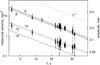Fig. 11 Dependence of the DIM variance ${\sigma }_{T,i}^2$ reduced to R = 1′ field size on the exposure T. The figure shows the individual estimates for each star (circle sizes are proportional to the star brightness) for the reduction with k = 6 (upper symbol sequence) and k = 12 (lower sequence); fit functions TB(k) (lines) for each k; theoretical dependence T−1. Dots are clustered in groups according to exposure in sky fields.

6.6 Change of DIM variance across the field of view

We especially emphasize that both the model and the observed DIM variances discussed in this article refer to a single target object indexed i = 0 near the field center, which corresponds to astrometry focused on precise measurement of a single binary system object. The estimate of DIM variance in other field points is of interest in works focused, for example, on astrometry of stellar clusters when science objects are spread over the field. We found the solution to this problem for a star at distance r off field from the center using the spectral description of the DIM process.

In the case concerned, we are interested in estimating the DIM for off-center stars indexed as i_off > 0 under the condition of using the least-squares transformation to the reference frame identical to that used for the reduction of the central i = 0 object, that is using the same projective matrix a (Sect. 5.1). The filter Q(q) for the relative shift of i_off star is computed with coefficients a_i in Eq. (10) equal, in this case, to elements a_ioff,i in the line i_off of the matrix a. Also, ρ_i in Eq. (10) are now the angular distances between i_off and the other i star. To derive the numerical solution, we adopted the CSD model, which matches well with the star distributions at the Galactic plane and the computed metric integrals I_r(k) as a function of off-center separation r. We found that I_r(k) for r till 0.1 R is within ±20% of the I_r=0(k) value in the field center. For off-center separations 0.3–0.5 R and k = 6, 10, 14, the excess of I_r(k) over I_r=0(k) increases respectively to 2.5, 1.5, and 1.2. Consequently, the DIM variance follows this change.

7 DIM in astrometric observations with other large seeing-limited telescopes

Using the methodology of DIM estimation based on the spectral description of this process and the availability of the vertical turbulence structure, we can compute variances ${\sigma }_{\mathrm{a}}^2$ expected for any other telescope location with any aperture D. We did it for the telescope of VLT size at the sea level and for the ELT at its actual location. In the first case, using Eq. (22) and adopting the same turbulent profile as for VLT, we obtained A₀ = 79.1 mpx² = 1.26 mas², or a factor 1.78 over that for VLT. Therefore, at the sea level for the VLT-size telescope, values a_R(k, R) are expected to be 1.3 times higher than those in Table 5.

Similar computations for the ELT located at 3046 m above the sea level and only 30 km away from VLT produced A₀ = 41.2 mpx² = 0.655 mas², or a factor 0.92 better than for VLT. Of course, the main improvement in the DIM variance follows from its large aperture D = 39 m due to the dependence ${\sigma }_{\mathrm{a}}^2\sim D^{-\nu }$, in accordance with Eq. (15). Using this dependence and adopting new A₀ value, we scaled a_R(k, R) from Table 5 known for VLT and thus derived the DIM variance for ELT (Table. 6). These amplitudes are on the order of ten better in comparison to those for VLT. In particular, we find that roughly a_R ≈ 2–5 μas for the R = 0.5′ field if transformation to the reference frame is made with orders k of the reduction polynomials from six to 14.

8 Conclusion

Astrometric reduction uses the least-squares transformation to the reference frame via coordinate polynomials of the order β, which is necessary to reduce geometric distortion of the field. At the same time, it mitigates the DIM effect caused by the atmospheric turbulence. We developed a model that adequately describes the image motion in the spectral domain, where instead of β, the use of the mode parameter k (Eq. (16)) is more convenient. This model allows us to translate the turbulence profile, if known, to the amplitude of the DIM displacements σ_a. A key quantity in this model is the metric integral I(d) (Eq. (13)), which numerically represents observational parameters (telescope diameter, field size, exposure, zenith angle, star distribution, brightness, seeing, background) as well as reduction parameters (β or k) and is computed for the distance d to the turbulent layer.

By prime examination, we have found that the measured (derived from observations) and the turbulent model DIM variances are best comparable when the latter are scaled roughly by a factor of τ₀ = 0.84, which is not a unit, probably due to the uncertainty in the turbulence profile. With this correction, the numeric value of ${\sigma }_a^2$ in zenith at a 30 s exposure is equal to the parameters A_c(k) in Table 2 for an imaginary star field with a unit I(d) computed at an effective distance d = 18 km to the turbulent layers. Values of A_c(k) depending on k (or β) vary between 0.69 and 0.77 mas².

We ran several tests to compare the model predictions with the observations. In the first test, we fit FORS2 measured DIM variances by a linear function of I and derived coefficients A_F(k), which by definition should be equal to A_c(k), but which are the observed quantities not dependent of the turbulence profile. The coefficients derived with FORS2 vary in the comparable range of 0.67–0.84 mas² (Table 3), depending on k also, with a clear correlation between both results (Fig. 7, Sect. 6.2). Thus, the model A_c(k) and the observational A_F(k) estimates are quite close.

In the second test, the measured variances were compared directly with those expected from the turbulent model (Fig. 8) and fit by a linear dependence with a scaling coefficient $\overline{\tau }(k)$. We derived that $\overline{\tau }(k)$ is in the range of 0.995–1.019 (Sect. 6.3). Thus, the correlation between the two estimates is excellent. A good agreement of the observations with a model is supported by the fact that the residuals of the least-squares fit obtained for these two tests have a Gaussian distribution with an rms very near its model expectation.

For another test, we investigated the dependence of the measured variances on the field size R and found that it follows an expected power dependence R^ν+p, which supports the Kolmogorov type of the turbulence (specified by p = 2/3) at effective altitudes 16–18 km. With this power law, we derived the DIM amplitude â_R(k) for FORS2 at R = 1′ field, the zenith, and the 30 s exposure for each k or β (Table 4). Using the turbulence profile (not using the actual FORS2 observations), we derived an alternative expression (Eq. (26)) of a similar structure but with coefficients a_F(k) estimated using turbulent data. Both coefficients, â_R(k) and a_F(k) shown in Table 4, are comparable to within the uncertainty limits.

In addition, we analyzed the dependence of the measured DIM variance ${\sigma }_{\mathrm{a}}^2$ on T (Fig. 11) and found that for any k, the observed power law is T⁻¹, as predicted by the model Eq. (38). In this test, estimates â_T(k) of the measured DIM variances at R = 1′ and T = 30 s match well with both turbulence model coefficients, a_F(k) and â_R(k), derived from observations in a different way (Table 4). The observational fact that ${\sigma }_{\mathrm{a}}^2$ follows an expected power law ~T⁻¹ means, furthermore, that the input of the static (time-constant) field deformations is negligible in comparison to that of the DIM for any k or β applied.

All of these tests demonstrated the agreement, to ~1%, between the observational and the model lines of the investigation. We emphasize that the spectral-based model is not limited to FORS2 only and that it can be generalized to predict ${\sigma }_a^2$ for other very large telescopes, including ELT (Sect. 7). Of course, our model estimates are restricted to telescopes that do not use adaptive optics.

Appendix A Calibration of the model and observed data

A.1 Rejection of outliers

In this study, DIM variance ${\sigma }_{\mathrm{a}}^2$ is found analyzing the differences $⟨{\mathrm{\Delta }}^2⟩-{\sigma }_{\mathrm{p}}^2-{\sigma }_{\mathrm{r}}^2$. The estimated value of ${\sigma }_{\mathrm{a}}^2$ therefore can be affected by the outlier measurements in the analyzed sample of Δ. The outlier distribution besides can depend on R producing a false increase of ⟨Δ²⟩ in a similar way affecting the ${\sigma }_{\mathrm{a}}^2$ dependence on R. The first impression is that the influence of outliers is minor, but really it is significant because the amplitude of ${\sigma }_{\mathrm{a}}^2$ is only 20–50% of ⟨Δ²⟩ for most stars at R = 2′, decreasing even to a few percent only at R ~ 1′. Thus even a minor bias in ⟨Δ²⟩ is amplified in the estimated value of ${\sigma }_{\mathrm{a}}^2$, especially at small R. Therefore we had to perform a special calibration of the residuals Δ to make its sample robust to the outliers rejection and then additionally scaling ⟨Δ²⟩ values to remove secondary bias caused by the rejection of outliers.

The outliers are removed usually at 3-sigma, or when |Δ| > 3σ_mod. This is well justified when the residuals are distributed by a Gaussian law. In our case, residuals Δ are expected to follow this distribution with a sigma parameter σ_mod because the main error components σ_p and σ_r are caused by fluctuations of the photon number, which are Gaussian by nature. To verify this, we computed normalized deviations u = Δ/σ_mod and formed the frequency distribution of u. It was made separately for primary and secondary P-stars, also, for each R, k and for data accumulated over all R. Surprisingly, accumulated distribution for all ~ 2.5 · 10⁶ residuals available was found to be really very much like the Gaussian, with no visual difference between the two P-star types or mode k. However, if the data are split separately for the narrow and wide R fields, the difference in distributions becomes essential. Thus, it reveals an excess at the distribution peak (u ~ 0) by 5–20% for narrow R and 5–10% depletion for the measurements with wide R. It means that the model uncertainties σ_mod are overestimated for narrow fields and underestimated for wide fields. This is due to insufficiently good error model, which makes the outlier rejection a little complicated.

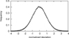Fig. A.1 Frequency distribution of the normalized positional residuals u′ obtained with the reduction mode k = 10 in an example sky field Nr.19 for the measurements reduced separately for narrow R < 360 px (triangles) and wide R > 840 px (crosses) fields. The normal law distribution is shown with a solid line.

We have found that any of the above partial distributions can be converted to being nearly Gaussian by introducing, instead of ${\sigma }_{\text{mod}}^2$, a new variance ${\sigma }_{\text{mod}}^2/{\alpha }^2$, where α is a constant (for some sky field and each R) scaling parameter, which makes the distribution of the deviations u′ = αΔ/σ_mod similar to the normal law distribution (Fig. A.1). Values α were derived by minimizing deviation between the measured and the normal distribution and they were obtained for each sky field, R, k, and separately for the target and reference stars. Most of values α are in the range of 0.9–1.1.

The sample distribution of deviations u′ is little dependent on R, k, and the star type (primary or reference P-star) in any sky field. This allowed us to perform rejection of outliers which exceed Zσ_mod/α at some cut level Z, not introducing a bias dependent on R. Thus we saved best dependence of the DIM variance on R. We applied levels Z = 2.5, 3, 4, Z = ∞ (no rejection) and whereupon abandoned the terms α.

The rejection procedure of course results in the decrease of the variance ⟨Δ²⟩ depending on Z. For a normal distribution this effect is easily estimated and can be corrected considering that after applying rejection at level Z the variance is ${\gamma }^2(Z)=\frac{1}{\sqrt{2\pi }}{\int }_{-Z}^Z{x}^2\exp (-x^2/2)dx<1$. Table A.1 provides values γ²(Z) for normal distribution with cut levels Z used in this investigation. Thus, assuming normal law distribution of the residuals Δ/σ_mod and having the variance ⟨Δ²⟩_Z computed at some rejection level Z, we can restore its unbiased variance $${⟨{\mathrm{\Delta }}^2⟩}_{\mathrm{\infty }}={⟨{\mathrm{\Delta }}^2⟩}_Z/{\gamma }^2(Z)$$(A.1)

correspondent to the full data sample (Z = ∞).

Similar numeric estimates of γ²(Z), showing the decrease of the variance, were computed for our measurements as the average of (Δ/σ_mod)² at each Z. We did it for all measurements of P-stars at all R, for each sky field, averaged over M exposures, and the resulting median for each k after normalization to a unit value at Z = 4 are given in Table A.1. These estimates match well those for the normal distribution mostly within ±0.02 and are little dependent on k. We consider this result acceptably good and as independent verification of the normal law distribution of single exposure residuals Δ. This means also validity of the correction (A.1) for our data. Finally, we applied rejection with Z = 3 only, recomputed ⟨Δ²⟩ as the weighted average of single frame variances Δ² and, using Eq. A.1, corrected these values with γ²(3) dependent on k (Table A.1).

A.2 Calibration of the error model components

According to Sect. A.1, Δ/σ_mod for single exposures follow a normal law distribution. It allows us to estimate uncertainty of ⟨Δ²⟩, which is the weighted average for a series of M exposures. It is known that a sum of squares of n normal values has a chi-square distribution with mathematical expectation n and a variance 2n. In our case, n = M because Δ² was defined as the average of this term in x and y. Therefore, mathematical expectation of ⟨Δ²⟩ is equal to ${\sigma }_{\text{mod}}^2$, and the uncertainty of this estimate is $${\sigma }_{⟨{\mathrm{\Delta }}^2⟩}=E{\sigma }_{mod}^2{M}^{-0.5},$$(A.2)

with E = 1 for exactly normal distribution of the residuals Δ. Ideally, the differences $⟨{\mathrm{\Delta }}^2⟩-{\sigma }_{\text{mod}}^2$ should have a zero expectation and nearly a Gaussian distribution with sigma parameter ${\sigma }_{⟨{\mathrm{\Delta }}^2⟩}$. Due to a large number M of images, a bias of the order of 5% in the model of ${\sigma }_{\text{mod}}^2$ is already detected as excessive value of deviations $⟨{\mathrm{\Delta }}^2⟩-{\sigma }_{\text{mod}}^2$. We searched for these inconsistencies and removed them by calibrations described below. This step of the study is quite necessary because inaccuracy in the initial ${\sigma }_{\text{mod}}^2$ model were found to mount to a few ${\sigma }_{⟨{\mathrm{\Delta }}^2⟩}$.

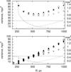Fig. A.2 Observed variance of the positional residuals ⟨Δ2⟩ (black dots) derived with an uncertainty of about 1–2 mpx2 as a function of the reference field radius for an example P-star in a sky field Nr.19. The initial model variance ${\sigma }_{\text{mod}}^2$ (crosses) and its components ${\sigma }_{\mathrm{p}}^2$ (dashed line), ${\sigma }_{\mathrm{r}}^2$ (dash-dotted), ${\sigma }_{\mathrm{a}}^2$ (dotted); updated (Sect. A.2.2) model variance ${\hat{\sigma }}_{\text{mod}}^2$ (circles). The star was reduced as a primary (upper panel) or a reference star (lower panel) using reduction mode k = 10.

In each sky field, we have at hand N_R = 11 estimates of the variances ⟨Δ²⟩ for each P-star reduced as a target, and yet (N_p − 1)N_R estimates for this star reduced as a reference object. Fig. A.2 illustrates typical change of the measured variance ⟨Δ²⟩ and its model components along the field size R for an example P-star in a sky field Nr.19. The upper panel corresponds to the primary status of this star and the error model Eq. 1. Deviations between the measured and the model variances is visually seen and largely exceed the uncertainty ${\sigma }_{⟨{\mathrm{\Delta }}^2⟩}$, which is only about 2 mpx² at R = 1000 px because of a large M = 2388.

The lower panel corresponds to the measurements of positional residuals of the same star i but now treated as a reference for nearby five primary P-stars, which results in a multiple set of ⟨Δ²⟩ and σ_r values shown in the plot. Unlike the upper plot, ⟨Δ²⟩ turns to zero at small R. This is a consequence of the fact that any errors in the photocenter measurements of a bright reference star cause bias in the transformation fit functions which results in equivalent change of the transformed positions and so to small residuals Δ.

A.2.1 Calibration withing sky fields

Figure A.2 demonstrates that model Eq. 5 represents the measured variance ⟨Δ²⟩ of the residuals far not perfect. In particular, this can be due to use of approximate parameters for the DIM taken from Lazorenko (2006). However, direct fit of a full set of ⟨Δ²⟩ by function Eq. 8 via parameters a and b leads to a large discrepancy between the measured and updated model variances. Besides, we derived strongly deviating estimates of a, b found separately for different sky fields, which is unacceptable. The problem therefore is in the approximate model values ${\sigma }_{\mathrm{p}}^2$ and ${\sigma }_{\mathrm{r}}^2$ which require correction at the level of ~10–20%. For instance, this may occur when the estimates (7) of ${\sigma }_{\mathrm{p}}^2$ are biased by errors in I_G flux, by deviations between the actual and the model star image shape, blending, other effects (Sect. 4).

We assumed that the components ${\sigma }_{\mathrm{p}}^2$ and ${\sigma }_{\mathrm{r}}^2$ require correction by a small scaling factor δ peculiar for each primary P-star. For instance, the actual value of ${\sigma }_{\mathrm{p}}^2$ for these stars i is ${\hat{\sigma }}_{\mathrm{p},i}^2=(1+{\delta }_{\mathrm{p},i}){\sigma }_{\mathrm{p},i}^2$ and the reference frame variance is ${\hat{\sigma }}_{\mathrm{r},i}^2=$ $(1+{\delta }_{\mathrm{r},i}){\sigma }_{\mathrm{r},i}^2+g_i$ with the scaling factor δ_r,i related to i-th primary star, which is constant for all R, and g_i is an offset. The DIM component was updated to the model ${\hat{\sigma }}_{\mathrm{a}}^2=a{R}^b$ with new constants fit values a and b estimated for each sky field. The calibration model contains 3N_p + 2 parameters (δ_p,i, δ_r,i, g_i, a and b) to be fit within each star field and which for primary stars have a simple structure: $${⟨{\mathrm{\Delta }}^2⟩}_i-{\sigma }_{\mathrm{p},i}^2-{\sigma }_{\mathrm{r},i}^2={\delta }_{\mathrm{p},i}{\sigma }_{\mathrm{p},i}^2+{\delta }_{\mathrm{r},i}{\sigma }_{\mathrm{r},i}^2+g_i+a{R}^b.$$(A.3)

We note that corrections δ_r,i refer to the case when the star i is a primary probing object. In the case of i-th star used as reference for i′ P-star, we first transformed the variance ${\sigma }_{\mathrm{r},i}^2$ (equal to ${\sigma }_{\mathrm{r},P_i>0}^2$ in Eq. 6) to the variance ${\sigma }_{\mathrm{r},P_i=0}^2$ which emulate reference frame noise related to the star i′ at location of i-th star. Because i and i′ are nearby stars, they have nearly same set of reference stars and the reference frame noise for these two stars with a status ‘primary’ is approximately equal. Thus ${\sigma }_{\mathrm{r},P_i=0}^2$ can serve as emulation ${\overline{\sigma }}_{\mathrm{r},i}^2$ of the reference noise ${\sigma }_{\mathrm{r},i}^2$ for i-th star in a ‘primary’ status. In terms of this variable, the model variance is expressed as ${\sigma }_{\text{mod}}^2={\sigma }_{\mathrm{p}}^2+{\sigma }_{\mathrm{a}}^2-{\overline{\sigma }}_{\mathrm{r},i}^2({\sigma }_{\mathrm{p}}^2+{\sigma }_{\mathrm{a}}^2)/({\sigma }_{\mathrm{p}}^2+{\sigma }_{\mathrm{a}}^2+{\overline{\sigma }}_{\mathrm{r},i}^2)$. Hence, we arrived at the calibration model: $${⟨{\mathrm{\Delta }}^2⟩}_i-{\sigma }_{\mathrm{p},i}^2+{\sigma }_{\mathrm{r},i}^2={\delta }_{\mathrm{p},i}\frac{\mathrm{\partial }{\sigma }_{mod}^2}{\mathrm{\partial }{\sigma }_{\mathrm{p}}^2}{\sigma }_{\mathrm{p},i}^2+{\delta }_{\mathrm{r},i}\frac{\mathrm{\partial }{\sigma }_{\mathrm{m}\mathrm{o}\mathrm{d}}^2}{\mathrm{\partial }{\overline{\sigma }}_r^2}{\overline{\sigma }}_{\mathrm{r},i}^2+g_i+a{R}^b,$$(A.4)

References

- Appenzeller, I., Fricke, K., Fürtig, W., et al. 1998, The Messenger, 94, 1 [NASA ADS] [Google Scholar]
- Butterley, T., Sarazin, M., Le Louarn, M., Osborn, J., & Farley, O. J. D. 2020, SPIE Conf. Ser., 11448, 114481W [NASA ADS] [Google Scholar]
- Cameron, P. B., Britton, M. C., & Kulkarni, S. R. 2009, AJ, 137, 83 [NASA ADS] [CrossRef] [Google Scholar]
- Clénet, Y., Gendron, E., Gratadour, D., Rousset, G., & Vidal, F. 2015, A&A, 583, A102 [NASA ADS] [CrossRef] [EDP Sciences] [Google Scholar]
- Conan, R., Avila, R., Sánchez, L. J., et al. 2003, in Rev. Mex. Astron. Astrofis. Conf. Ser., 19, eds. I. Cruz-Gonzalez, R. Avila, & M. Tapia, 31 [Google Scholar]
- Dali Ali, W., Ziad, A., Berdja, A., et al. 2010, A&A, 524, A73 [NASA ADS] [CrossRef] [EDP Sciences] [Google Scholar]
- Irwin, M. J. 1985, MNRAS, 214, 575 [NASA ADS] [Google Scholar]
- Lazorenko, P. F. 2002, A&A, 396, 353 [NASA ADS] [CrossRef] [EDP Sciences] [Google Scholar]
- Lazorenko, P. F. 2006, A&A, 449, 1271 [NASA ADS] [CrossRef] [EDP Sciences] [Google Scholar]
- Lazorenko, P. F., & Lazorenko, G. A. 2004, A&A, 427, 1127 [NASA ADS] [CrossRef] [EDP Sciences] [Google Scholar]
- Lazorenko, P. F., Mayor, M., Dominik, M., et al. 2009, A&A, 505, 903 (Paper I) [NASA ADS] [CrossRef] [EDP Sciences] [Google Scholar]
- Lazorenko, P. F., Sahlmann, J., Ségransan, D., et al. 2014, A&A, 565, A21 [NASA ADS] [CrossRef] [EDP Sciences] [Google Scholar]
- Le Louarn, M., Hubin, N., Sarazin, M., & Tokovinin, A. 2000, MNRAS, 317, 535 [NASA ADS] [CrossRef] [Google Scholar]
- Lindegren, L., Klioner, S. A., Hernández, J., et al. 2021, A&A, 649, A2 [EDP Sciences] [Google Scholar]
- Masciadri, E., Lascaux, F., & Fini, L. 2013, MNRAS, 436, 1968 [NASA ADS] [CrossRef] [Google Scholar]
- Mendez, R. A., Silva, J. F., & Lobos, R. 2013, PASP, 125, 580 [NASA ADS] [CrossRef] [Google Scholar]
- Osborn, J., Wilson, R. W., Sarazin, M., et al. 2018, MNRAS, 478, 825 [CrossRef] [Google Scholar]
- Pott, J.-U., Rodeghiero, G., Riechert, H., et al. 2018, SPIE Conf. Ser., 10702, 1070290 [NASA ADS] [Google Scholar]
- Pravdo, S. H., & Shaklan, S. B. 1996, ApJ, 465, 264 [NASA ADS] [CrossRef] [Google Scholar]
- Rodeghiero, G., Arcidiacono, C., Pott, J.-U., et al. 2021, J. Astron. Telescopes Instrum. Syst., 7, 035005 [NASA ADS] [Google Scholar]
- Sahlmann, J., Lazorenko, P. F., Ségransan, D., et al. 2014, A&A, 565, A20 [NASA ADS] [CrossRef] [EDP Sciences] [Google Scholar]
- Sahlmann, J., Burgasser, A. J., Martín, E. L., et al. 2015a, A&A, 579, A61 [NASA ADS] [CrossRef] [EDP Sciences] [Google Scholar]
- Sahlmann, J., Lazorenko, P. F., Ségransan, D., et al. 2015b, A&A, 577, A15 [NASA ADS] [CrossRef] [EDP Sciences] [Google Scholar]
- Sahlmann, J., Lazorenko, P. F., Bouy, H., et al. 2016, MNRAS, 455, 357 [NASA ADS] [CrossRef] [Google Scholar]
- Sarazin, M. S., Osborn, J., Chacon-Oelckers, A., et al. 2017, in Optics in Atmospheric Propagation and Adaptive Systems XX, eds. K. U. Stein, & S. Gladysz, Vol. 10425, International Society for Optics and Photonics (SPIE), 104250B [Google Scholar]
- Schöck, M., Do, T., Ellerbroek, B. L., et al. 2014, SPIE Conf. Ser., 9148, 91482L [Google Scholar]
- Taheri, M., McConnachie, A., Turri, P., et al. 2022, AJ, 163, 187 [NASA ADS] [CrossRef] [Google Scholar]
- Trippe, S., Davies, R., Eisenhauer, F., et al. 2010, MNRAS, 402, 1126 [NASA ADS] [CrossRef] [Google Scholar]
All Tables
Parameters Ac(k), ac(k) for CSD and aF(k) for FORS2 fields based on the turbulence profile at a 30 s exposure.
Differential image motion amplitude σa [μas] at 30 s exposure in the zenith for a typical FORS2 star field in the Galactic plane.