| Issue |
A&A
Volume 606, October 2017
|
|
|---|---|---|
| Article Number | A140 | |
| Number of page(s) | 13 | |
| Section | Stellar atmospheres | |
| DOI | https://doi.org/10.1051/0004-6361/201731422 | |
| Published online | 25 October 2017 | |
Spectroscopic properties of a two-dimensional time-dependent Cepheid model
I. Description and validation of the model
1 Zentrum für Astronomie der Universität Heidelberg, Landessternwarte, Königstuhl 12, 69117 Heidelberg, Germany
2 Max-Planck-Institut für Astronomie (MPIA), Königstuhl 17, 69117 Heidelberg, Germany
e-mail: vasilyev@mpia-hd.mpg.de
3 Department of Physics and Astronomy, Uppsala University, Regementsvägen 1, Box 516, 75120 Uppsala, Sweden
4 Zentrum für Astronomie der Universität Heidelberg, Astronomisches Recheninstitut, Mönchhofstr. 12-14, 69120 Heidelberg, Germany
5 INAF–Osservatorio Astronomico di Capodimonte, via Moiariello 16, 80131 Napoli, Italy
Received: 22 June 2017
Accepted: 28 August 2017
Context. Standard spectroscopic analyses of Cepheid variables are based on hydrostatic one-dimensional model atmospheres, with convection treated using various formulations of mixing-length theory.
Aims. This paper aims to carry out an investigation of the validity of the quasi-static approximation in the context of pulsating stars. We check the adequacy of a two-dimensional time-dependent model of a Cepheid-like variable with focus on its spectroscopic properties.
Methods. With the radiation-hydrodynamics code CO5BOLD, we construct a two-dimensional time-dependent envelope model of a Cepheid with Teff = 5600 K, log g = 2.0, solar metallicity, and a 2.8-day pulsation period. Subsequently, we perform extensive spectral syntheses of a set of artificial iron lines in local thermodynamic equilibrium. The set of lines allows us to systematically study effects of line strength, ionization stage, and excitation potential.
Results. We evaluate the microturbulent velocity, line asymmetry, projection factor, and Doppler shifts. The microturbulent velocity, averaged over all lines, depends on the pulsational phase and varies between 1.5 and 2.7 km s-1. The derived projection factor lies between 1.23 and 1.27, which agrees with observational results. The mean Doppler shift is non-zero and negative, −1 km s-1, after averaging over several full periods and lines. This residual line-of-sight velocity (related to the “K-term”) is primarily caused by horizontal inhomogeneities, and consequently we interpret it as the familiar convective blueshift ubiquitously present in non-pulsating late-type stars. Limited statistics prevent firm conclusions on the line asymmetries.
Conclusions. Our two-dimensional model provides a reasonably accurate representation of the spectroscopic properties of a short-period Cepheid-like variable star. Some properties are primarily controlled by convective inhomogeneities rather than by the Cepheid-defining pulsations. Extended multi-dimensional modelling offers new insight into the nature of pulsating stars.
Key words: radiative transfer / stars: variables: Cepheids / methods: numerical / stars: atmospheres / convection / stars: oscillations
© ESO, 2017
1. Introduction
Cepheid variable stars play an important role in astronomy. In cosmological applications they are standard candles to measure Galactic and extragalactic distances with unprecedented precision (Riess et al. 2016) due to a remarkable relation between the pulsation period and their intrinsic luminosity (the Leavitt law: Leavitt 1908; Leavitt & Pickering 1912). The period-luminosity relation can provide measurements of the distance up to approximately 30 Mpc. Despite the overall successful application of the period-luminosity relation, its universality has been one of the most debated issues concerning Cepheids in the last few decades (see e.g. Marconi et al. 2005; Romaniello et al. 2008; Marconi 2009; Marconi et al. 2010; Bono et al. 2010; Wielgorski et al. 2017, and references therein). Indeed, if the chemical composition affects Cepheid pulsation properties, this systematic effect will reflect on the associated extragalactic distance scale.
On the other hand, the chemical composition of Cepheids can provide information on the chemodynamical evolution of galaxies. Abundances and abundance ratios of many chemical elements can be measured from Cepheid spectra to derive their distribution in different environments within the Galaxy and beyond. For instance, abundance gradients in the Galactic disk for 25 chemical elements (from carbon to gadolinium) were measured (Andrievsky et al. 2002a,b, 2004; Luck et al. 2003; Lemasle et al. 2007).
The standard method for determining Cepheid atmospheric parameters and abundances is based on one-dimensional plane-parallel hydrostatic stellar model atmospheres. The models cover a wide range of the stellar parameters (e.g., Kurucz 1992) allowing one to estimate the effective temperature, surface gravity, and microturbulent velocity, which change with pulsational phase, as well as the phase-independent abundances (see e.g. Luck & Andrievsky 2004; Kovtyukh et al. 2005; Andrievsky et al. 2005; Luck et al. 2008). Physically, the pulsational period is of the same order as the dynamical timescale defined by the sound travel time across the star. The relaxation time for mechanical disturbances caused by pulsational waves in comparison with the pulsational period characterizes the deviation from hydrostatic conditions. For a Cepheid model with a ten-day period, deviations from hydrostatic conditions are expected to be on the level of a few percent (Gautschy 1987); this is also the case for thermal deviations. From this perspective one would expect that the standard approach should work rather satisfactorily.
Dynamical non-linear stellar models of pulsating stars restricted to one spatial dimension (1D) have a long history (see e.g. Christy 1962, 1964; Cox et al. 1966; Stellingwerf 1982; Bono & Stellingwerf 1994; Bono et al. 1999; Marconi et al. 2005; Smolec & Moskalik 2008). In those works, the convective flux was modelled using a 1D time-dependent theory of convection and a characteristic scale length over which convection mixes mass, typically taken proportionally to the pressure scale height. Models were aimed to reproduce the light and radial velocity curves and location of the instability strip in the Hertzsprung-Russel diagram. Moreover, Fokin (1991), Fokin et al. (1996), and Fokin & Gillet (1997) used 1D models to perform spectral synthesis calculations to investigate shock propagation and turbulence in Cepheid atmospheres.
Recently, two-dimensional (2D) hydrodynamic simulations of Cepheid envelopes were performed by Mundprecht et al. (2013, 2015), including comparisons to convection prescriptions commonly applied in 1D modelling. Their simulations show that the strength of the convection zone varies significantly over the pulsation period and exhibits a phase shift relative to the variations in radius. To successfully match this multi-dimensional result by a 1D static, or even time-dependent convection model, appears challenging. The authors conclude that significant improvements are needed to make predictions based on 1D models more robust and to improve the reliability of conclusions on the convection–pulsation coupling drawn from them. Multi-dimensional simulations can provide guidelines for developing descriptions of convection then applied in traditional 1D modelling. Freytag et al. (2017) used the CO5BOLD radiation-hydrodynamics code to produce an exploratory grid of global three-dimensional (3D) “star-in-a-box” models of the outer convective envelope and the inner atmosphere of asymptotic giant branch (AGB) stars to study convection, pulsations, and shock waves and their dependence on stellar and numerical parameters. For these stars with low-effective temperature and gravity, the lifetime of convective cells is comparable to the pulsational timescale, which makes it possible to model pulsations, but the spatial resolution is not high enough for detailed spectral synthesis. In summary, calculation of a grid of multi-dimensional Cepheid atmosphere models is a sizable computational problem due to the presence of different spatial and temporal scales.
Here we present the – to our knowledge – first spectroscopic investigation of a 2D envelope models of a Cepheid-like variable where the non-local and time-dependent nature of convection is included from first principles. Radiative transfer is treated non-locally, albeit in grey approximation. Our intention is to demonstrate that the model is able to capture relevant features of the Cepheid physics despite the employed approximations. In Sect. 2 we describe the model, in Sect. 3 we study its spectroscopic properties. Specifically, we derive the microturbulent velocity from the 2D model and report on the methodology behind its derivation, as well as describe the behaviour of the line equivalent widths and asymmetries. In Sect. 4 we discuss line shifts and give an interpretation of the residual spectroscopic line-of-sight radial velocity. A derivation of the projection factor (p-factor), which is a key parameter in the Baade-Wesselink method of the distance determination to Cepheids, is discussed in Sect. 5. Section 6 lists our conclusions.
2. Description of the model
Radiation-hydrodynamics simulations of a short-periodic Cepheid-like variable employing grey radiative transfer were calculated with the CO5BOLD code (Freytag et al. 2012) in 2D Cartesian geometry. The models gt56g20n01 to gt56g20n04 have a nominal effective temperature of Teff = 5600 K, and a constant depth-independent gravitational acceleration of log g = 2. The pulsation period of the Cepheid model comes out to ≈2.8 days. The simulations use an equidistant spatial grid of Nx × Nz = 600 × 500 (model gt56g20n01) to 580 (gt56g20n04) points along the horizontal and vertical direction, respectively. The corresponding geometrical size of the largest model is lx × lz = 1.12 × 1012 cm ×5.4 × 1011 cm. The size of the grid cells is 1.88 × 109 cm ×9.38 × 108 cm. For the flow, impenetrable boundaries are imposed at the top and bottom of the domain; the side boundaries are periodic. A radiative flux according to the nominal effective temperature is prescribed at the bottom. Radiation can pass unimpeded through the top of the modelled box. The chemical composition of the model is close to solar. Specifically, the hydrogen abundance is log ϵH = 12.0, helium abundance log ϵHe = 11.0, silicon abundance log ϵSi = 7.5, and iron abundance log ϵFe = 7.46.
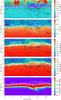 |
Fig. 1 Entropy (top panel), temperature, pressure, density, and He ii ionization fraction nHe ii/ (nHe i + nHe ii + nHe iii) (bottom panel) as function of the horizontal and vertical coordinates at time t = 1.40 × 10⁷ s, which corresponds to an expanding phase. Pseudo-streamlines are shown as black solid lines. Surfaces of constant Rosseland optical depth are shown by white lines: τR = 1 (solid line), τR = 10-2 (dashed line), τR = 10-4 (dashed-dotted line). |
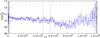 |
Fig. 2 Initial evolution in time of the bolometric flux of the model. Pulsations set in at t ≈ 106 s. Dotted lines indicate the time interval without pulsations for which spectral synthesis calculations were performed. |
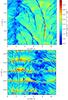 |
Fig. 3 Spatio-temporal evolution of the emergent intensity directed in vertical direction (μ = 1). The upper panel shows a time interval when pulsations have not set in (model gt56g20n01), the bottom panel a time interval with fully developed pulsations (model gt56g20n04). Time, spatial, and colour scales are identical for both panels. |
Figure 1 depicts images of entropy, temperature, pressure, density, and He ii ionization fraction at an instance in time during the expansion phase as a function of geometrical coordinates. Convection produces horizontal inhomogeneities so that surfaces of constant optical depth are not flat. The pulsating model exhibits strong shocks. Low density gas is falling down from above and collides with expanding photospheric and sub-photospheric material. At the so-formed accretion front, density and pressure jump by up to three orders of magnitude. We checked that such jumps cannot be simply understood as the result of the Rankine-Hugoniot (adiabatic) shock conditions but further factors must play a role. As evident from the lines of constant optical depth, line formation typically takes place in the region between the accretion front and optical depth unity.
We emphasize that the construction of the model was a numerical challenge. The largest obstacle is the extremely small numerical time step imposed by the short radiative relaxation time on a time-explicit scheme (for a detailed discussion, see Mundprecht et al. 2013). It enforces the restriction to 2D models, at the moment. In addition, strong pulsations can tend to cause an imbalance between mass in- and outflow resulting in a net time-averaged mass flow across the top boundary. To avoid it, the closed top boundary was chosen. However, the closed top boundary enhances strong artificial velocity gradients close to the boundary. To decrease the influence of them on dynamics of optically thin regions, we applied an artificial drag force in a number of grid layers close to the top, reducing the velocities by a certain fraction per time interval. This numerical approach impacts on the dynamics of the line formation regions of strong lines, which like the Ca triplet form at the outer atmosphere near the chromosphere. To avoid the impact of boundary effects we consider lines that are forming deeper in the range log τR = −3...0.
The model shows self-excited fundamental mode pulsations starting from initially plane-parallel static conditions (adding random small amplitude disturbances to break the symmetry). The initial evolution in time of the bolometric flux of the model is shown in Fig. 2. Pulsations set in at around ≈ 6 × 10⁶ s. They are excited by the κ-mechanism (Eddington 1917; Zhevakin 1963). In particular, around 4% of the radiative flux  is spent to ionize hydrogen, which is fully ionized for Rosseland optical depth τR> 1, due to the steep temperature gradient, and is largely neutral for τR< 1. The main driver of pulsations is the region of singly ionized helium (see bottom panel in Fig. 1). The thickness of the He ii ionization zone varies; He ii ionization stores and releases 16% of the radiative energy passing the layer during a pulsational cycle.
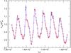 |
Fig. 4 Model light curve in terms of the emergent bolometric flux. Red circles mark the instances in time for which a spectral synthesis was performed. |
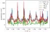 |
Fig. 5 The total acceleration dv/ dt + g0 experienced by a (Lagrangian) mass element close to optical depth unity as a function of time, where g0 is the constant gravitational acceleration. Coloured lines show the contributions to the pressure gradient by the gas pressure pgas, and turbulent pressure pt, as well as the resulting sum p = pgas + pt balanced by the total acceleration. |
Before pulsations have set in, the flow evolution is mostly governed by convection. Regions with up- and down-flows at the photosphere affect the outgoing radiation field. The spatio-temporal evolution of the emergent intensity (in vertical direction, μ = 1) when pulsations have not set in is shown in the top panel of Fig. 3. The intensity map exhibits a typical convective pattern. In particular, convection generates a few large-scale down-flows, which exist for long timescales > 106 s. Smaller-scale down-flows of cooled gas have a tendency to get “sucked” into the dominant larger-scale flows. Down-flows correlate with lower intensities, the bluer regions in Fig. 3.
The intensity map for later phases when pulsations have set in is shown in the bottom panel of Fig. 3. The convective pattern now consists of a dominant large-scale down-flow in the right part of the intensity map, and small-scale flows that evolve independently. For the given atmospheric parameters and assuming a mass of roughly 5 M⊙, one can expect around 300 granulation cells on the visible hemisphere. The mass was motivated from inspection of the PAdova and TRieste Stellar Evolution Code (PARSEC) evolutionary tracks (Bressan et al. 2012).
The phase of maximum compression roughly coincides with the phase of maximum brightness (see also Fig. 4). Maximum brightness is not reached at exactly the same time at all locations but depends slightly on the morphology of the convective surface flow. For instance, in the large down-flow maximum brightness is reached slightly earlier than in the neighbouring regions. This illustrates the impact of horizontal inhomogeneities on the pulsations.
Preferentially during phases of maximum brightness, which almost coincide with the maximum compression, convective down-flows are generated. This is a sign of the action of the convective instability. The efficiency of convection depends on the gravitational acceleration g0, and the growth timescale of the convective instability τconv is proportional 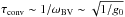 , where ωBV is the Brunt-Väisälä frequency. The time evolution of the acceleration a of a pseudo-Lagrangian mass element following the mean vertical mass motion close to the photosphere is shown in Fig. 5. The model itself is based on an Eulerian description of the flow field from which one can transform to a pseudo-Lagrangian reference frame. During the reversal of the direction of motion at the phase of maximum compression, a photospheric pseudo-Lagrangian mass element experiences an acceleration of ≈ (1.0...2.5)g0. In total it experiences an effective acceleration of geff = a + g0 ≈ (2.0...3.5)g0, which amplifies the convective instability and also leads to high convective velocities. One can see in Fig. 5 that the turbulent pressure pt adds a significant contribution to the total pressure gradient, which is equal to the effective gravity: −∇(pgas + pt) /ρ = a + g0.
A 1D mean model, which is the result of horizontal averaging of the full 2D model at fixed geometrical height, was used to analyze the pulsational velocity and radiation flux. The radial velocity curve of a layer with the Rosseland optical depth τR = 2/3 shown in Fig. 6 was calculated by cubic spline interpolation of the vertical velocity component of the mean 1D model. The amplitude of the radial velocity is V ≈ 20 km s-1, which is quite typical for a Cepheid (Groenewegen 2013). The non-zero mean vertical velocity of the optical surface is the consequence of the presence of convective fluctuations, large amplitudes of pulsations and a non-linearity of opacities as a function of the temperature. A word on sign conventions: in the CO5BOLD simulations the vertical axis is directed toward the observer so that a positive vertical velocity corresponds to a blueshift. However, normally the spectroscopic convention for the radial velocity is used in this work, where a blueshift corresponds to a negative velocity.
A light curve in terms of the bolometric flux is shown in Fig. 4. Red circles mark instances in time for which a spectral synthesis was performed with Linfor3D1 (Gallagher et al. 2016). The light curve covers a time interval with fully developed pulsations covering six periods. For each 2D snapshot, Linfor3D solves the radiative transfer equation along three inclined angles for two azimuthal angles, which are lying in the xz-plane, and along the vertical direction. To accelerate the spectral synthesis one can sub-sample the model structure along the x-axis. Tests taking each and every third grid point along the x-axis were performed for a line Fe iλ6003 Å. Equivalent widths for these cases come out very similar: WΔnx = 1 = 109.8 mÅ and WΔnx = 3 = 111.2 mÅ. Due to the similarity, the computationally less demanding sub-sampled case is used in this paper.
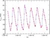 |
Fig. 6 Vertical (radial) velocity of a layer at fixed Rosseland optical depth τR = 2/3. Here, a positive velocity corresponds to a blueshift. |
2.1. Convective noise
Observed light and radial velocity curves of Cepheids are typically smooth, and show a high degree of similarity from cycle to cycle. The model light curve in Fig. 4 and the radial velocity curve in Fig. 6 do not at all exhibit these properties. Amplitude and shape of the curves change significantly during the pulsations. This is the result of convection, which adds statistical fluctuations to the velocity and thermal structure of the model. The fluctuations in the pressure gradients shown in Fig. 5 are a clear illustration of this “convective noise”. The convective noise appears so prominent in our light and velocity curves since our model represents only a small part of the surface of a Cepheid. The fluctuations would decrease if we increased the spatial extent of the model, or could take recourse to many realizations of the stellar surface with independent convective but coherent pulsational properties. However, both options would demand prohibitively expensive additional simulations. In the following we try to mitigate the effects of the fairly low resulting signal-to-noise ratio by adequate procedures when extracting simulation properties. As a side, we note that the cycle-to-cycle variations in Cepheids recently reported by Anderson (2016) might be an imprint of the residual convective noise after averaging over the full stellar disk. However, it is difficult to extrapolate the convective noise properties of our calculated model to a long-period Cepheid. According to the period-mean gravity relation (Gough et al. 1965), it requires approximately a factor of ten lower gravitational acceleration for a 35-day pulsation period, which changes the convective timescale, velocities, characteristic sizes, and lifetimes of convective cells.
2.2. Effects of the Cartesian geometry and grey radiative transfer
Our Cepheid model has Cartesian geometry while the structure of a real Cepheid is more accurately represented by a spherical geometry. We want to estimate the impact of the Cartesian geometry here.
In Cepheids the radius changes due to the pulsations are of the order of ≈ 10%, which corresponds to a change in the stellar volume of  , where the subscript s indicates a spherical geometry. For the planar (subscript p) geometry adopted here, the change is
  . For adiabatic pulsations, there is a corresponding difference of the temperature change
 ![\hbox{$\Delta \frac{\Delta T}{T} = \left[ \left( \frac{\Delta V}{V} \right)_\mathrm{s} - \left( \frac{\Delta V}{V} \right)_\mathrm{p} \right] \times (\gamma_\mathrm{ad}-1)=0.2 \times (\gamma_\mathrm{ad}-1)$}](/articles/aa/full_html/2017/10/aa31422-17/aa31422-17-eq58.png) , where γad is the adiabatic exponent, which is equal to 5/3 for an ideal monatomic gas. One would arrive at the same conclusion if one considered an atmosphere with a fixed thickness during the pulsations. Hence, the different geometry leads to a temperature difference of ≈ 13%. This is significant, and eventually means noticeable changes in the conditions for line formation. However, as we will see in a moment, the temperature does not follow adiabatic changes but is rather controlled by radiation. Radiative properties differ less between the geometries since the thickness of the atmosphere is still rather small in a Cepheid – significantly less than its radius change during the pulsational cycle.
, where γad is the adiabatic exponent, which is equal to 5/3 for an ideal monatomic gas. One would arrive at the same conclusion if one considered an atmosphere with a fixed thickness during the pulsations. Hence, the different geometry leads to a temperature difference of ≈ 13%. This is significant, and eventually means noticeable changes in the conditions for line formation. However, as we will see in a moment, the temperature does not follow adiabatic changes but is rather controlled by radiation. Radiative properties differ less between the geometries since the thickness of the atmosphere is still rather small in a Cepheid – significantly less than its radius change during the pulsational cycle.
 |
Fig. 7 Comparison of the characteristic radiative relaxation time and the actual timescales on which temperature changes happen for three Lagrangian mass elements in the atmosphere. The elements are located in the line formation region at time-averaged optical depths log τR = 0.04,−1.95,−2.75. |
One can argue that using grey radiative transfer in the model is far from realistic and may lead to different qualitative changes of the thermal structure during the pulsations in comparison to the case of frequency-dependent (non-grey) radiative transfer. Especially the characteristic timescale of radiative relaxation, which is defined as the time for reaching radiative equilibrium conditions in the atmosphere, depends on the opacity treatment. To derive characteristic timescales we follow Ludwig et al. (2002). With the assumption that the geometrical size of a thermal disturbance is equal to the local pressure scale height, the radiative relaxation timescale in Eddington approximation can be written as:  (1)where cp denotes the specific heat at constant pressure, σ Stefan-Boltzmann’s constant, χ the Rosseland opacity, and τdis = χρHp the optical size of the assumed temperature disturbance.
The actual characteristic time of change of the temperature tT of a mass element in the atmosphere model can be calculated as  (2)where dT/ dt is a rate of the temperature change. This timescale depends on local fluctuations of the temperature due to the presence of disturbances generated by convection or pulsations. The pulsational period tpuls characterizes the global change of the thermal structure during the pulsations.
Figure 7 shows the timescales as a function of time for three Lagrangian mass elements in the atmosphere, which are lying in the line formation region with time-averaged optical depths log τR = 0.04, −1.95, −2.75. The properties of the mass elements were calculated from the 1D mean model. The radiative relaxation timescale is shorter than both the pulsational period and the characteristic time of the temperature change in the line formation regions, except in phases of maximum compression, during which for the highest parts of formation regions the timescale is comparable with the period of pulsations. One can see that the characteristic time of change of the temperature does not depend much on the optical depth for the line formation region and it has the same order as the pulsational period. The radiative timescales have been evaluated under simplifying assumptions, and should therefore be taken as order of magnitude estimates only. Our choice of the disturbance size is rough. One might argue that the size of horizontal disturbances generated by convection is a more appropriate length scale, and typically amounts to a few pressure scale heights. Even with 10HP, trad does not change much since the optical depth is already quite low (in the optically thin limit the radiative timescale is independent of the size of the disturbance). We conclude that radiation is able to keep the temperature structure close to radiative equilibrium – consistent with actual modelling results for the line formation region. For non-grey radiative transfer, the radiative timescale is shorter (see e.g. Ludwig et al. 2002). The stronger coupling between radiation and matter in the non-grey case would maintain radiative equilibrium conditions even more effectively. However, since the grey radiative transfer is already capable of doing so, the main difference to the non-grey case would be the lack of line blanketing and back warming, which is rather modest. One also expects in the non-gray case smaller temperature fluctuations in the photosphere, and the mean temperature gradient might be steeper. We conclude that our 2D Cartesian model provides fairly realistic estimates of the thermal conditions in the line formation region.
2.3. Relating velocity and luminosity amplitudes
Kjeldsen & Bedding (1995) derived a universal relation between the luminosity (δL/L)bol and velocity vosc amplitudes of oscillations for many classes of oscillating stars using linear theory and observational data:  (3)The relation was calibrated using β and δ Cephei, δ Scuti, and RR Lyrae stars. For a given Teff and vosc, one can predict the luminosity amplitude (δL/L)pred and compare it with the observed luminosity amplitude. For the 2D Cepheid model, the predicted luminosity amplitude (δL/L)pred ≈ 0.375 for the vosc ≈ 20 km s-1 and Teff = 5600 K. The “observed” luminosity amplitude of the model is ≈ 0.35. Both of them are in good agreement with the result of Kjeldsen & Bedding (1995) within the 1σ scatter.
3. Spectroscopic properties
Spectral properties are directly accessible to observation, and we want to characterize our model in terms of its spectroscopic characteristics. Microturbulence is an important “side parameter” in a standard spectroscopic analysis. Gillet et al. (1999) derived the microturbulence velocity curve of δ Cep using 1D non-linear non-adiabatic pulsating models. Perhaps not surprisingly, the microturbulent velocity turns out to change with pulsational phase. Here we attempt a first pilot study of the microturbulence derived from a multi-dimensional Cepheid model.
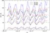 |
Fig. 8 Equivalent widths obtained from the 2D model as a function of time for lines of Fe i λ5500 Å with excitation energies of Ei = 1,3,5 eV (coloured solid lines). Different oscillator strengths were used for each excitation energy to cover a range of equivalent widths from 10 mÅ to 130 mÅ at starting time, as apparent by the four groups of three lines each. |
3.1. Microturbulence
Our estimate of the microturbulent velocity is based on the method described in Steffen et al. (2013). The procedure is as follows: for a spectral line, a spectral synthesis is performed using the 2D thermal structure with different velocity fields: (i) using the original 2D velocity field v2D; and (ii) replacing the 2D hydrodynamic velocity field with an isotropic, depth independent microturbulent velocity ξmic as in a case of classical 1D spectral synthesis. The microturbulent velocity for the considered spectral line at each instance in time is defined by the requirement EW(v2D) = EW(ξmic). In practice, we calculated EW(ξmic) for a small grid of ξmic and interpolated in this grid to the desired EW(v2D). This method allows us to determine a microturbulent velocity for each individual line. It is clear that it differs from the classical procedure where one considers a set of weak and strong lines. However, besides having the virtue of being able to assign a microturbulence to a single line, the procedure applied here is perhaps the cleanest possible way to derive a microturbulence if one wants to actually associate the microturbulence with a velocity field providing the non-thermal line broadening.
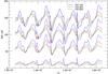 |
Fig. 10 Equivalent widths as a function of time for lines of Fe i λ5500 Å with excitation energy Ei = 1,3,5 eV. The EWs are calculated by replacing the 2D hydrodynamic velocity field by an isotropic, depth-independent Gaussian microturbulent velocity of ξmic = 3 km s-1. |
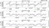 |
Fig. 11 Microturbulent velocity Vmic as a function of time for lines of Fe i λ5500 Å with Ei = 1,3,5 eV. log gf1 (strongest line) > log gf2> log gf3> log gf4 (weakest line). |
A set of fictitious neutral and singly ionized iron lines with fixed wavelength λ = 5500 Å but different line strengths and excitation potentials was used to conduct a systematic survey of the microturbulent velocity as a function of time. The excitation energies for Fe i lines were Ei = 1,3,5 eV; for Fe ii they were Ei = 1,3,5,10 eV. Oscillator strengths were chosen for each excitation energy Ei so as to cover a range of equivalent widths from 10 mÅ to 130 mÅ in steps of 20 mÅ for the initial instance in time at step (i).
Based on the 2D model, equivalent widths (EWs) for a set of Fe i and Fe ii lines as a function of time in step (i) are shown in Figs. 8 and 9. Both groups of these lines, Fe i and Fe ii, show a modulation of the equivalent width with pulsational phase for both strong and weak lines. The amplitude of the EW variation is bigger for Fe i than for Fe ii, for the same initial line strengths. Lines of the Fe i and Fe ii with bigger line strength have higher amplitude of the variation of EWs. The overall behaviour can be directly understood from the different temperature sensitivities of the lines in the two different ionization stages. Besides a roughly periodic variation of the equivalent widths, there is a stochastic component stemming from the convective noise in the model.
For step (ii), the spectral synthesis was calculated using a depth-independent isotropic Gaussian microturbulent velocity in the range ξmic = 0.5−6.0 km s-1 to cover the range usually found in studies of Cepheids (Luck et al. 1998; Andrievsky et al. 2002c). A plot with the result of the spectral synthesis of the Fe iλ5500 Å with ξmic = 3 km s-1 is shown in Fig. 10. The increase of the microturbulent velocity leads to an increase of the EW. Strong lines are very sensitive to variations of the microturbulence.
The calculation of ξmic by the requirement EW(v2D) = EW(ξmic) was done with a third order spline interpolation. The microturbulence as a function of time for Fe i and Fe ii lines is shown in Figs. 11 and 12. We note that the calculated synthetic spectra have infinite resolution and signal-to-noise, which allows us to assign a microturbulence even to the weakest lines of our sample. The microturbulence exhibits a clear modulation with the pulsational phase with an amplitude of ≈ 0.5...1.0 km s-1 and a certain degree of randomness due to convection. Around photometric phase 0.9 before maximum light the microturbulent velocity curve exhibits distinct peaks. These peaks coincide with the moment when the model is near its minimum radius. This is qualitatively in agreement with the temporal behaviour of turbulent velocities as measured by Borra & Deschatelets (2017) using an autocorrelation technique. One has to keep in mind that their turbulent velocities include contributions from rotation as well as macro- and microturbulence. The absolute value of the microturbulent velocity is 1.0...4.0 km s-1, which is less than observed in short period Cepheids ≈ 1.5...5.0 km s-1 (Andrievsky et al. 2001). The microturbulence slightly decreases with increasing excitation potential, and it averaged over all lines varies with pulsational cycle between 1.5 and 2.7 km s-1.
There are several reasons why our model may fall somewhat short of the observed values: (a) our procedure to derive the microturbulence does not exactly mimic the observational procedure; (b) our selection of lines differs noticeably from the set of lines used in the observations; (c) our model harbours indeed a low microturbulence. In particular, limited spatial resolution leads to a systematically low ξmic (Steffen et al. 2013). Nevertheless, we are content that at least on the whole the microturbulence in the 2D model follows the evidence from observations.
3.2. Spikes in the EW(t) curves
Both results of the spectral synthesis coming from step (i) with the full 2D model and step (ii) with the microturbulent velocity show that the EWs depend on the pulsational phase. The amplitude of the variation of the EW is larger for stronger lines. Occasionally, the EWs from steps (i) and (ii) show sharp spikes. This behaviour is obviously not related to the 2D velocity field, because the spikes still appear in step (ii) where the velocity field is replaced by a constant microturbulent velocity. The change of the thermal structure plays the key role here, which is illustrated in Fig. 13. At time t = 1.466 × 10⁷ s, the equivalent width of the Fe i lines in Fig. 8 has a sharp maximum because the temperature gradient is steeper than at previous and subsequent times in the line formation region with Rosseland optical depth τR = 10-2...1. The spikes of the equivalent width of the Fe i lines show up during phases of maximum compression. The EWs of the Fe ii lines show additional spikes due to the deep location of the line formation regions. The impact of convection on the Fe ii line formation regions is more than for similar regions of Fe i lines. Lines forming very deep might also reach into the region of the badly resolved sub-photospheric temperature jump. Unfortunately, in this important region, where convection starts, the numerical resolution is not quite sufficient.
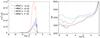 |
Fig. 13 Time dependence of the non-normalized line equivalent width contribution functions of the weakest Fe i λ5500 Å Ei = 1 eV line (left panel) and the temperature profiles (right panel). The contribution functions and the temperature profiles for each instance in time are depicted in corresponding colours. |
3.3. Line asymmetry
Sabbey et al. (1995) devised a method to measure the asymmetry of lines. They found that for classical Cepheids the observed line asymmetry is a function of the pulsational phase and correlates with the position of the line core. The asymmetry of a spectral line profile was determined from the difference and sum of the areas of the red and blue profile halves: (Sred−Sblue) /Stot. Two different methods were used to determine the line core position:
-
1.
fitting a Gaussian to the whole line profile;
-
2.
fitting a parabola to the line core below 70% of the continuum level.
The results of the spectral syntheses show a complex multicomponent structure of the line profiles. However, we found that 30% is a reasonable part of the line to limit systematic effects related to the complex line profile on the determination of the position of the line core. Fe i Ei = 1 eV and Fe ii Ei = 1 eV line profiles for the strongest case as a function of the photometric phase are shown in Fig. 14. The photometric phase zero coincides with maximum light of the light curve. Synthetic line profiles for most phases have a multicomponent structure.
Following Sabbey et al. (1995), the line asymmetry was considered as a function of the dynamical phase φd (see Fig. 15). The dynamical phase zero coincides with the moment of the velocity reversal from contraction to expansion in the photosphere. The amplitude of the line asymmetry variation is ≈ 0.2...0.3, which on average is larger than that found in observational data. Sabbey et al. measured the amplitude of variations of the line asymmetry to ≈ 0.1...0.3. Nevertheless, the time dependence of the line asymmetry has the same behaviour for the model and observations (Sabbey et al. 1995). The 2D model provides only very limited spatial statistics. We expect that the higher degree of smoothing when averaging over the full stellar disc is reducing line asymmetries and variations in line core position, largely removing the part that is stemming from convection-related inhomogeneities. However, there is clear indication that weak lines show systematically larger variations of the line asymmetry independent of the method used to measure the line core position.
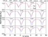 |
Fig. 14 Fe iEi = 1 eV and Fe ii Ei = 1 eV line profiles for the strongest case as a function of photometric phase. Photometric phase φp zero coincides with maximum light. |
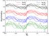 |
Fig. 15 Line asymmetries of the Fe i λ5500 Å with Ei = 3 eV as a function of the dynamical phase φd. Line strength changes in order of oscillator strength with log gf1> log gf2> log gf3 > log gf4. Dynamical phase zero coincides with the velocity reversal from contraction to expansion in the photosphere. The line asymmetry curves are shifted by 0.5 dex relative to each other for clarity. |
3.4. Line-depth ratio and the effective temperature
The ratio of depths of the spectral lines with high- and low-excitation potentials is a very sensitive temperature indicator (Gray & Johanson 1991; Gray 1994). This powerful method for estimating the effective temperature was applied by Kovtyukh et al. (2006) and Gray & Brown (2001) to giant stars, and by Kovtyukh & Gorlova (2000) and Kovtyukh (2007) to supergiants. The calibration of Kovtyukh & Gorlova (2000) was used by Andrievsky et al. (2005), Luck & Andrievsky (2004), and Kovtyukh et al. (2005) to determine the effective temperatures of Cepheids over a range of periods from three to ten days.
Kovtyukh (2007) obtained around 130 different line pair relations for estimating the effective temperatures of supergiants as a function of line depth ratio. As one example, we investigated the often used pair Fe iλ6085.27 Å and Si iλ6155.14 Å. The effective temperature as a function of the Fe i λ6085.27 Å to Si iλ6155.14 Å line depth ratio lFeI/lSiI in the 2D model is shown in Fig. 16 for two different solar-scaled abundances of Fe and Si. To calculate the photometric phase φp the radial velocity curve was fitted by a harmonic function A × sin(ωt + φo).
The slope of the function Teff(lFe i/lSi i) is somewhat steeper than in the case of supergiants (Kovtyukh 2007). It is possible that for Cepheids with periods shorter than three days, dynamical effects in the atmosphere are stronger. Again, cycle-to-cycle variations due to the convective noise are clearly discernible. Interestingly, maximum Teff is compatible with range of values for the line depth ratio, making the overall relation not unique, and a small line depth ratio can hint towards a low or high Teff. However, such an ambiguity can be easily resolved if the phase of observation is roughly known. All in all we can confirm that the method of line depth ratios works for our 2D model. However, we see more fine-structure than a simple unique relation. Moreover, the calibration for supergiants does not fit perfectly the data of our short period Cepheid model.
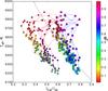 |
Fig. 16 Effective temperature as function of the Fe i λ6085.27 Å and Si i λ6155.14 Å line depth ratio for two different abundances. Big circles connected by a blue line mark a case with + 0.4 dex abundance increase for Si and Fe; small circles connected by a red line mark a case with −0.4 dex. The colour of the circles indicates the photometric phase φp. The dashed curve depicts the calibration of Kovtyukh (2007) for supergiants. |
4. Interpretation of the “K-term”
As was emphasized by Sabbey et al. (1995), different methods of measuring the Doppler shift of absorption lines yield systematically different results. For perfectly symmetric line profiles, measuring the line-core position by using a parabolic fit to the core region (i), a Gaussian fit to the whole profile (ii), or the centroid velocity (iii), given by the first moment of the spectral line profile, yields identical results. The advantage of the third method is its independence of rotation and turbulent line broadening (Burki et al. 1982; Nardetto et al. 2006). However, the absorption line profiles of Cepheids are asymmetric. The three methods can thus lead to different results, but fortunately – as it turns out – the qualitative picture does not depend on the specific choice. The line profiles of Fe i 1 Ei = 1 eV are shown for two extreme cases of the minimum and maximum of the spectroscopic radial velocity and measured Doppler shifts with these methods in Fig. 17. For the blue shifted asymmetric line, the third method gives the smallest Doppler shift. The difference to a Gaussian fit is ≈ 5 km s-1. For the red shifted case, the line profile is less asymmetric and all methods give almost the same Doppler velocity. From this experiment we expect that the moment method gives smaller blue-shifts, which is confirmed later (see Fig. 21). We remark that we neglect the gravitational redshift in our discussion, which is ≲100 m s-1 for Cepheids.
In the following the spectroscopic radial velocity is based on measurement of the Doppler shift of the absorption line using both these methods.
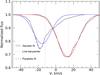 |
Fig. 17 The line profiles of Fe i 1 Ei = 1 eV for two extreme cases (black) of the minimum (blue) and maximum (red) of the spectroscopic radial velocity and measured Doppler shifts of the the line-core position by using a parabolic fit to the core region, by using a Gaussian fit to the whole profile and the centroid velocity. |
The radial velocity does not show noticeable differences of the amplitude and phase shift for different excitation potentials and oscillator strengths (see Fig. 18). In contrast, the mean radial velocity ⟨ v ⟩ t shown in Figs. 19, 23, and 20, which is the result of an averaging over six full cycles, exhibits dependencies on excitation potential and line strength. Additionally, the path conservation integral is not equal to zero, which is a basic assumptions in the Baade-Wesselink method (Gautschy 1987): 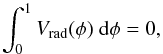 (4)where the integral is calculated over a complete pulsation cycle. Path conservation is used to derive the centre-of-mass velocity Vγ (or γ-velocity ) of a pulsating star from the above integral of the radial velocity via the condition
  .
.
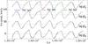 |
Fig. 18 Radial velocities as a function of time obtained by measuring the Doppler shift of Fe i λ5500 Å Ei = 1 eV (blue), 3 eV (red), 5 eV (green) line cores using parabolic fits. Four different line strengths are shown whose EWs are ordered according to their oscillator strength log gf1 > log gf2 > log gf3 > log gf4. The velocity curves are shifted by 40 km s-1 relative to each other for clarity. |
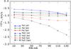 |
Fig. 19 Time-averaged radial velocities ⟨v⟩t of Fe i and Fe ii lines as a function of their EW. The measurement of the Doppler shift is based on parabolic fits of the line core deeper than 70% of the total line depth. |
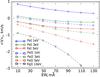 |
Fig. 21 Time-averaged radial velocities ⟨v⟩t of Fe i and Fe ii lines as a function of their EW. The measurement of the Doppler shift is based on the barycenter of the spectral line. |
Observational evidence for the presence of a residual systematic velocity has existed for around 70 years (Parenago & Kukarkin 1947; Stibbs 1956; Wielen 1974; Sabbey et al. 1995). The kinematic behaviour of Cepheids (Wilson et al. 1991; Pont et al. 1994) shows a “K-term”, which is a residual line-of-sight velocity of the order −2 km s-1 (toward us) between the measured (spectroscopically) centre-of-mass velocity and the Galactic rotational velocity derived from the kinematics of stellar populations. Sabbey et al. (1995) presumed that this residual velocity is related to the varying depth of the photospheric line-forming region with pulsational phase. Based on very high quality the High Accuracy Radial velocity Planet Searcher (HARPS) observations and careful methodology, Nardetto et al. (2009) showed that the γ-velocities are linearly correlated with the line asymmetry AVγ = a0A + b0 and intrinsic properties of Cepheids. The residual γ-velocity (or K-term) averaged over eight stars was measured to b0 = 1.0 ± 0.2 km s-1.
The K-term can be affected by both pulsations and convection. To better understand the contributions of the two processes, 2D model snapshots were taken for an initial phase of the simulation run when pulsations had not set in yet. Spectral syntheses of Fe i (Ei = 1,3,5 eV) and Fe ii (Ei = 1,3,5,10 eV) lines as in a case of pulsations were calculated for 100 2D snapshots between (4.5−5.8) × 106 s. The Doppler shift of the lines was measured using parabolic fits limited to residual fluxes of 30% above the line core, and Gaussian fits of the entire line profiles. The time-averaged radial velocities ⟨ v ⟩ t based on the three methods are shown in Figs. 22–24. As was mentioned before, the method of fitting does not change the qualitative picture and Figs. 22–24 show a similar dependence of the mean radial velocity on excitation potential, line strength, and ionization degree. Fe ii lines with high excitation potential are forming in deeper layers of the atmosphere than in the case of the Fe i. This indicates that the effect of convection is stronger than the effect of pulsations.
Comparing the mean velocities before and after the pulsations have set in using both Gaussian and parabolic fits and the first moment of the spectral line profile (as shown in Figs. 23, 20, 19, 22, 24, and 21) led us to conclude that convection is the main contributor to the residual velocity. The contribution of pulsations is not essential, and only provides a spreading with line properties leaving the averages largely intact. Therefore, we interpret the γ-velocity as the Cepheid version of the convective blueshift present in all late-type stars with convective outer envelopes. The derived values of the residual γ-velocity varies between 1.0 and 0.5 km s-1 dependent on method. They are close to the observed K-term for Cepheids (Nardetto et al. 2009). The dependence of the centroid velocity on the line asymmetry in the first moment method leads to a smaller residual velocity of 0.5 km s-1 (see Fig. 17). A parabolic fit to the core region gives ≈ 1 km s-1 of the residual γ-velocity. The method is closer to the cross-correlation method applied for radial velocity measurements with the standard G2 mask with the HARPS spectrograph, because the widths of the “lines” of the mask is 3 km s-1. This is much narrower than the width of lines in a Cepheid, and effectively leads to a determination of the line position given by the line core. The period of the 2D model is 2.8 days whereas typically Cepheids have longer periods and lower surface gravities. Spectroscopic observations of Nardetto et al. (2006) indicate that for longer periods and lower log g the more vigorous convective motions produce larger residual γ-velocities.
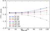 |
Fig. 22 Time-averaged radial velocities from line core fitting when pulsations have not set in. |
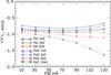 |
Fig. 23 Time-averaged radial velocities from Gaussian fitting when pulsations have not set in. |
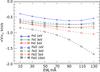 |
Fig. 24 Time-averaged barycenter radial velocities when pulsations have not set in. |
5. Projection factor obtained from the 2D model
The projection factor p (also p-factor) is a key quantity in the Baade-Wesselink method for determining the distances of Cepheids. The method relates the spectroscopically measured radial velocities of a Cepheid to interferometrically measured angular-diameters (Sasselov & Karovska 1994; Kervella et al. 2004), or classically to their brightness, by using a calibrated surface-brightness-colour relation (Barnes & Evans 1976; Fouque & Gieren 1997; Gieren et al. 1989; Storm et al. 2011). The method assumes the radius is defined at a specific location in the stellar atmosphere, for example, at an optical depth τ = 2/3. The change of the radius is  , where the pulsation velocity vpuls is the velocity of optical layers corresponding to the optical depth τ = 2/3. The projection factor p converts the spectroscopic radial velocity to a pulsational velocity: vpuls = p × vrad. Spectroscopic radial velocities include effects related to two kinds of integration over the stellar surface layers: horizontally, the effects of limb-darkening, and vertically, the effects of velocity gradients in the line-forming region.
The impact of limb-darkening and atmospheric expansion on the p-factor was first studied by Eddington (1926) and Carroll (1928). Parsons (1972), using a model atmosphere with uniform expansion, numerically determined the p-factor to be between 1.31 and 1.34, depending on the width of a line. Many attempts were made to estimate and calibrate the p-factor from high-resolution spectroscopic observations (Nardetto et al. 2004, 2007, 2009, 2013, 2017; Breitfelder et al. 2015; Neilson et al. 2012; Breitfelder et al. 2016). Nardetto et al. (2007) identified three effects affecting the projection factor: the geometrical effect, the velocity gradient within the atmosphere, and the relative motion of a layer of given optical depth with respect to a corresponding fixed Lagrangian mass element.
Our Cepheid model provides information about the pulsating velocity vpuls(τR = 2/3). The photospheric radius Rph(τR = 2/3) was calculated with a cubic spline interpolation using data of the mean 1D model. The pulsating velocity is vpuls = dRph/ dt, which was calculated for each instance in time over six full periods. The projection factor is the slope of the curve vpuls = p × vrad + vo, which is shown in Fig. 25 for the line Fe i Ei = 1 eV and three different line strengths. We implemented the fitting to deal with the substantial amount of convective noise present in the model data. Depending on line strength the p-factor varies between 1.23 and 1.27, which agrees with estimates from the literature (Nardetto et al. 2009). Additionally, within the given noise level, Fig. 25 shows the absence of a hysteresis-like behaviour between the pulsational and radial velocities as was found when investigating the relation between effective temperature and line depth ratio (Fig. 16).
The fitting parameter vo is related to the K-term. The presence of residual γ-velocity shifts the curve vpuls = p × vrad + vo to negative radial velocities along the horizontal axis so that K = −vo/p. The derived K-term from the linear fits as a function of line strength is shown in Fig. 26.
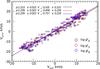 |
Fig. 25 Pulsational velocity as a function of the radial velocity, estimated by Gaussian fits of the whole Fe i Ei = 1 eV line profiles. Colours show different line strengths: the strongest line is depicted in black, the weakest in blue. The slope of the linear regression is the p-factor. |
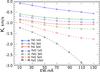 |
Fig. 26 Residual velocity or K-term derived by linear fits of the curve vpuls = p × vrad + vo and K = −vo/p for different line strengths and excitation potentials. The spectroscopic radial velocity is measured by Gaussian fitting. |
From the physical point of view, the pulsational velocity is related to the motion of mass elements in the atmosphere during the pulsations. One can estimate the pulsational velocity using the velocities of mass elements close to the photosphere, and thereby calculate the projection factor. The variation of the geometric vertical coordinate of a layer in the photosphere with τR = 2/3 and a Lagrangian mass element is shown in Fig. 27. The pulsational velocity of these layers is shown in Fig. 28. The pseudo-Lagrangian velocity of the mass element is almost equal to the velocity of the optical depth surface τR = 2/3 in the photosphere. That means that in our model we find the same projection factor for the pseudo-Lagrangian velocity, or the velocity of a layer of given optical depth (in the photosphere).
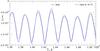 |
Fig. 27 Vertical geometric coordinate of a layer in the photosphere with τR = 2/3, and the corresponding pseudo-Lagrangian mass element as a function of time. |
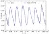 |
Fig. 28 Pulsational velocities of a layer in the photosphere with τR = 2/3, and of the corresponding pseudo-Lagrangian mass element as a function of time. |
6. Conclusions and final remarks
A pilot study of spectroscopic properties of a multi-dimensional Cepheid model was conducted. We arrive at the following conclusions:
-
1.
The 2D model shows self-excited pulsations due to theκ-mechanism with a 2.8-day period. It reproduces the observedrelation between the brightness and radial velocity amplitudes ofpulsating stars (Kjeldsen & Bedding 1995).
-
2.
We find a net mean shift of the spectrum of the model Cepheid by −0.5...−1 km s-1 which is a significant fraction of the observed residual line-of-sight velocity seen in the Cepheid population.
-
3.
We interpret this shift as the convective blueshift familiar from non-pulsating late-type stars. It is possible that multi-dimensional models with lower surface gravity (more similar to typical Cepheids) give higher convective and, eventually, higher residual velocities bringing the models closer to observations. This needs to be investigated further.
-
4.
The microturbulent velocity, derived for individual iron lines, shows a modulation with pulsational phase and depends on the line properties. When averaged over all lines, it varies between 1.5 and 2.7 km s-1 over the pulsational cycle. This is somewhat lower than the velocity obtained in classical analyses with 1D hydrostatic atmosphere models (Andrievsky et al. 2001). Reasons for this shortcoming may be the limited spatial resolution of the model, or the different methodology used in the determination of the microturbulent velocity. However, around photometric phase 0.9 before maximum light, the microturbulent velocity curve exhibits distinct peaks. This is qualitatively in agreement with the temporal behaviour of turbulent velocities in Cepheids as measured by Borra & Deschatelets (2017) using an autocorrelation technique.
-
5.
Line asymmetries show a behaviour that is qualitatively similar to observations. However, limited statistics makes it difficult to perform more quantitative comparisons.
-
6.
The projection factor derived from the 2D model lies between 1.23 and 1.27, and agrees with observations (Nardetto et al. 2009).
Taken together we find a reasonable correspondence between the model and observed properties of Cepheid variables. This is far from self-evident considering the computational problems one faces when trying to simulate a Cepheid envelope exhibiting self-excited pulsations together with violent atmospheric dynamics. The 2D geometry together with detailed spectral syntheses sets our model apart from most previous modelling works. It allowed us to study the impact of convective inhomogeneities, which turned out to be important for some spectroscopic properties – here in particular for the K-term – and, as we will present in a follow-up paper, for the determination of elemental abundances. At least in the minds of the authors, this leads to a shift in the way we should look at Cepheid variables. While their defining property of being pulsating giant stars following a period-luminosity relation is still perhaps their most important single characteristic, now convection comes into focus. Its importance has always been masked by the giant stars’ prominent pulsations.
Acknowledgments
V.V. would like to thank Dr. Anish Amarsi for valuable comments on the draft. H.G.L. and B.L. acknowledge financial support by the Sonderforschungsbereich SFB 881 “The Milky Way System” (subprojects A4, A5) of the German Research Foundation (DFG). The radiation-hydrodynamics simulations were performed at the Pôle Scientifique de Modélisation Numérique (PSMN) at the École Normale Supérieure (ENS) in Lyon.
References
- Anderson, R. I. 2016, MNRAS, 463, 1707 [NASA ADS] [CrossRef] [Google Scholar]
- Andrievsky, S. M., Kovtyukh, V. V., Luck, R. E., et al. 2001, VizieR Online Data Catalog: J/A+A/381/32 [Google Scholar]
- Andrievsky, S. M., Kovtyukh, V. V., Luck, R. E., et al. 2002a, A&A, 381, 32 [NASA ADS] [CrossRef] [EDP Sciences] [Google Scholar]
- Andrievsky, S. M., Kovtyukh, V. V., Luck, R. E., et al. 2002b, A&A, 392, 491 [NASA ADS] [CrossRef] [EDP Sciences] [Google Scholar]
- Andrievsky, S. M., Kovtyukh, V. V., Luck, R. E., et al. 2002c, VizieR Online Data Catalog: J/A+A/392/494 [Google Scholar]
- Andrievsky, S. M., Luck, R. E., Martin, P., & Lépine, J. R. D. 2004, A&A, 413, 159 [NASA ADS] [CrossRef] [EDP Sciences] [Google Scholar]
- Andrievsky, S. M., Luck, R. E., & Kovtyukh, V. V. 2005, AJ, 130, 1880 [NASA ADS] [CrossRef] [Google Scholar]
- Barnes, T. G., & Evans, D. S. 1976, MNRAS, 174, 489 [NASA ADS] [CrossRef] [Google Scholar]
- Bono, G., & Stellingwerf, R. F. 1994, ApJS, 93, 233 [NASA ADS] [CrossRef] [Google Scholar]
- Bono, G., Marconi, M., & Stellingwerf, R. F. 1999, ApJS, 122, 167 [NASA ADS] [CrossRef] [Google Scholar]
- Bono, G., Caputo, F., Marconi, M., & Musella, I. 2010, ApJ, 715, 277 [NASA ADS] [CrossRef] [Google Scholar]
- Borra, E. F., & Deschatelets, D. 2017, MNRAS, 470, 4732 [NASA ADS] [CrossRef] [Google Scholar]
- Breitfelder, J., Kervella, P., Mérand, A., et al. 2015, A&A, 576, A64 [NASA ADS] [CrossRef] [EDP Sciences] [Google Scholar]
- Breitfelder, J., Mérand, A., Kervella, P., et al. 2016, A&A, 587, A117 [NASA ADS] [CrossRef] [EDP Sciences] [Google Scholar]
- Bressan, A., Marigo, P., Girardi, L., et al. 2012, MNRAS, 427, 127 [NASA ADS] [CrossRef] [Google Scholar]
- Burki, G., Mayor, M., & Benz, W. 1982, A&A, 109, 258 [NASA ADS] [Google Scholar]
- Carroll, J. A. 1928, MNRAS, 88, 548 [NASA ADS] [CrossRef] [Google Scholar]
- Christy, R. F. 1962, ApJ, 136, 887 [NASA ADS] [CrossRef] [Google Scholar]
- Christy, R. F. 1964, Rev. Mod. Phys., 36, 555 [NASA ADS] [CrossRef] [Google Scholar]
- Cox, A. N., Brownlee, R. R., & Eilers, D. D. 1966, ApJ, 144, 1024 [NASA ADS] [CrossRef] [Google Scholar]
- Eddington, A. S. 1917, The Observatory, 40, 290 [NASA ADS] [Google Scholar]
- Eddington, A. S. 1926, The Internal Constitution of the Stars (Cambridge: Cambridge University Press) [Google Scholar]
- Fokin, A. B. 1991, MNRAS, 250, 258 [NASA ADS] [CrossRef] [Google Scholar]
- Fokin, A. B., & Gillet, D. 1997, A&A, 325, 1013 [NASA ADS] [Google Scholar]
- Fokin, A. B., Gillet, D., & Breitfellner, M. G. 1996, A&A, 307, 503 [NASA ADS] [Google Scholar]
- Fouque, P., & Gieren, W. P. 1997, A&A, 320, 799 [NASA ADS] [Google Scholar]
- Freytag, B., Steffen, M., Ludwig, H.-G., et al. 2012, J. Comput. Phys., 231, 919 [Google Scholar]
- Freytag, B., Liljegren, S., & Höfner, S. 2017, A&A, 600, A137 [NASA ADS] [CrossRef] [EDP Sciences] [Google Scholar]
- Gallagher, A. J., Steffen, M., Caffau, E., et al. 2017, Mem. Soc. Astron. It., 88, 82 [NASA ADS] [Google Scholar]
- Gautschy, A. 1987, Vist. Astron., 30, 197 [Google Scholar]
- Gieren, W. P., Barnes, III, T. G., & Moffett, T. J. 1989, ApJ, 342, 467 [NASA ADS] [CrossRef] [Google Scholar]
- Gillet, D., Fokin, A. B., Breitfellner, M. G., Mazauric, S., & Nicolas, A. 1999, A&A, 344, 935 [NASA ADS] [Google Scholar]
- Gough, D. O., Ostriker, J. P., & Stobie, R. S. 1965, ApJ, 142, 1649 [NASA ADS] [CrossRef] [Google Scholar]
- Gray, D. F. 1994, PASP, 106, 1248 [NASA ADS] [CrossRef] [Google Scholar]
- Gray, D. F., & Brown, K. 2001, PASP, 113, 723 [NASA ADS] [CrossRef] [Google Scholar]
- Gray, D. F., & Johanson, H. L. 1991, PASP, 103, 439 [NASA ADS] [CrossRef] [Google Scholar]
- Groenewegen, M. A. T. 2013, A&A, 550, A70 [NASA ADS] [CrossRef] [EDP Sciences] [Google Scholar]
- Kervella, P., Nardetto, N., Bersier, D., Mourard, D., & Coudé du Foresto, V. 2004, A&A, 416, 941 [NASA ADS] [CrossRef] [EDP Sciences] [Google Scholar]
- Kjeldsen, H., & Bedding, T. R. 1995, A&A, 293, 87 [NASA ADS] [Google Scholar]
- Kovtyukh, V. V. 2007, MNRAS, 378, 617 [NASA ADS] [CrossRef] [Google Scholar]
- Kovtyukh, V. V., & Gorlova, N. I. 2000, A&A, 358, 587 [NASA ADS] [Google Scholar]
- Kovtyukh, V. V., Andrievsky, S. M., Belik, S. I., & Luck, R. E. 2005, AJ, 129, 433 [NASA ADS] [CrossRef] [Google Scholar]
- Kovtyukh, V. V., Soubiran, C., Bienaymé, O., Mishenina, T. V., & Belik, S. I. 2006, MNRAS, 371, 879 [NASA ADS] [CrossRef] [Google Scholar]
- Kurucz, R. L. 1992, in The Stellar Populations of Galaxies, eds. B. Barbuy, & A. Renzini (Dordrecht: Kluwer Academy Publisher), IAU Symp., 149, 225 [Google Scholar]
- Leavitt, H. S. 1908, Annals of Harvard College Observatory, 60, 87 [Google Scholar]
- Leavitt, H. S., & Pickering, E. C. 1912, Harvard College Observatory Circular, 173, 1 [Google Scholar]
- Lemasle, B., François, P., Bono, G., et al. 2007, A&A, 467, 283 [NASA ADS] [CrossRef] [EDP Sciences] [Google Scholar]
- Luck, R. E., & Andrievsky, S. M. 2004, AJ, 128, 343 [NASA ADS] [CrossRef] [MathSciNet] [Google Scholar]
- Luck, R. E., Moffett, T. J., Barnes, III, T. G., & Gieren, W. P. 1998, AJ, 115, 605 [NASA ADS] [CrossRef] [Google Scholar]
- Luck, R. E., Gieren, W. P., Andrievsky, S. M., et al. 2003, A&A, 401, 939 [NASA ADS] [CrossRef] [EDP Sciences] [Google Scholar]
- Luck, R. E., Andrievsky, S. M., Fokin, A., & Kovtyukh, V. V. 2008, AJ, 136, 98 [Google Scholar]
- Ludwig, H.-G., Allard, F., & Hauschildt, P. H. 2002, A&A, 395, 99 [NASA ADS] [CrossRef] [EDP Sciences] [Google Scholar]
- Marconi, M. 2009, Mem. Soc. Astron. It., 80, 141 [NASA ADS] [Google Scholar]
- Marconi, M., Musella, I., & Fiorentino, G. 2005, ApJ, 632, 590 [NASA ADS] [CrossRef] [Google Scholar]
- Marconi, M., Musella, I., Fiorentino, G., et al. 2010, ApJ, 713, 615 [NASA ADS] [CrossRef] [Google Scholar]
- Mundprecht, E., Muthsam, H. J., & Kupka, F. 2013, MNRAS, 435, 3191 [NASA ADS] [CrossRef] [Google Scholar]
- Mundprecht, E., Muthsam, H. J., & Kupka, F. 2015, MNRAS, 449, 2539 [NASA ADS] [CrossRef] [Google Scholar]
- Nardetto, N., Fokin, A., Mourard, D., et al. 2004, A&A, 428, 131 [NASA ADS] [CrossRef] [EDP Sciences] [Google Scholar]
- Nardetto, N., Mourard, D., Kervella, P., et al. 2006, A&A, 453, 309 [NASA ADS] [CrossRef] [EDP Sciences] [Google Scholar]
- Nardetto, N., Mourard, D., Mathias, P., Fokin, A., & Gillet, D. 2007, A&A, 471, 661 [NASA ADS] [CrossRef] [EDP Sciences] [Google Scholar]
- Nardetto, N., Gieren, W., Kervella, P., et al. 2009, A&A, 502, 951 [NASA ADS] [CrossRef] [EDP Sciences] [Google Scholar]
- Nardetto, N., Mathias, P., Fokin, A., et al. 2013, A&A, 553, A112 [NASA ADS] [CrossRef] [EDP Sciences] [Google Scholar]
- Nardetto, N., Poretti, E., Rainer, M., et al. 2017, A&A, 597, A73 [NASA ADS] [CrossRef] [EDP Sciences] [Google Scholar]
- Neilson, H. R., Nardetto, N., Ngeow, C.-C., Fouqué, P., & Storm, J. 2012, A&A, 541, A134 [NASA ADS] [CrossRef] [EDP Sciences] [Google Scholar]
- Parenago, P. P., & Kukarkin, B. V. 1947, Peremennye zvezdy, 3, 206 [Google Scholar]
- Parsons, S. B. 1972, ApJ, 174, 57 [NASA ADS] [CrossRef] [Google Scholar]
- Pont, F., Mayor, M., & Burki, G. 1994, A&A, 285, 415 [NASA ADS] [Google Scholar]
- Riess, A. G., Macri, L. M., Hoffmann, S. L., et al. 2016, ApJ, 826, 56 [NASA ADS] [CrossRef] [Google Scholar]
- Romaniello, M., Primas, F., Mottini, M., et al. 2008, A&A, 488, 731 [NASA ADS] [CrossRef] [EDP Sciences] [Google Scholar]
- Sabbey, C. N., Sasselov, D. D., Fieldus, M. S., et al. 1995, ApJ, 446, 250 [NASA ADS] [CrossRef] [Google Scholar]
- Sasselov, D., & Karovska, M. 1994, ApJ, 432, 367 [NASA ADS] [CrossRef] [Google Scholar]
- Smolec, R., & Moskalik, P. 2008, Acta Astron., 58, 193 [NASA ADS] [Google Scholar]
- Steffen, M., Caffau, E., & Ludwig, H.-G. 2013, Mem. Soc. Astron. It. Suppl., 24, 37 [Google Scholar]
- Stellingwerf, R. F. 1982, ApJ, 262, 330 [NASA ADS] [CrossRef] [Google Scholar]
- Stibbs, D. W. N. 1956, MNRAS, 116, 453 [NASA ADS] [Google Scholar]
- Storm, J., Gieren, W., Fouqué, P., et al. 2011, A&A, 534, A94 [NASA ADS] [CrossRef] [EDP Sciences] [Google Scholar]
- Wielen, R. 1974, A&AS, 15,1 [NASA ADS] [Google Scholar]
- Wielgorski, P., Pietrzynski, G., Gieren, W., et al. 2017, ApJ, 842, 116 [NASA ADS] [CrossRef] [Google Scholar]
- Wilson, T. D., Barnes, III, T. G., Hawley, S. L., & Jefferys, W. H. 1991, ApJ, 378, 708 [NASA ADS] [CrossRef] [Google Scholar]
- Zhevakin, S. A. 1963, ARA&A, 1, 367 [NASA ADS] [CrossRef] [Google Scholar]
All Figures
|
Fig. 1 Entropy (top panel), temperature, pressure, density, and He ii ionization fraction nHe ii/ (nHe i + nHe ii + nHe iii) (bottom panel) as function of the horizontal and vertical coordinates at time t = 1.40 × 10⁷ s, which corresponds to an expanding phase. Pseudo-streamlines are shown as black solid lines. Surfaces of constant Rosseland optical depth are shown by white lines: τR = 1 (solid line), τR = 10-2 (dashed line), τR = 10-4 (dashed-dotted line). |
| In the text | |
|
Fig. 2 Initial evolution in time of the bolometric flux of the model. Pulsations set in at t ≈ 106 s. Dotted lines indicate the time interval without pulsations for which spectral synthesis calculations were performed. |
| In the text | |
|
Fig. 3 Spatio-temporal evolution of the emergent intensity directed in vertical direction (μ = 1). The upper panel shows a time interval when pulsations have not set in (model gt56g20n01), the bottom panel a time interval with fully developed pulsations (model gt56g20n04). Time, spatial, and colour scales are identical for both panels. |
| In the text | |
|
Fig. 4 Model light curve in terms of the emergent bolometric flux. Red circles mark the instances in time for which a spectral synthesis was performed. |
| In the text | |
|
Fig. 5 The total acceleration dv/ dt + g0 experienced by a (Lagrangian) mass element close to optical depth unity as a function of time, where g0 is the constant gravitational acceleration. Coloured lines show the contributions to the pressure gradient by the gas pressure pgas, and turbulent pressure pt, as well as the resulting sum p = pgas + pt balanced by the total acceleration. |
| In the text | |
|
Fig. 6 Vertical (radial) velocity of a layer at fixed Rosseland optical depth τR = 2/3. Here, a positive velocity corresponds to a blueshift. |
| In the text | |
|
Fig. 7 Comparison of the characteristic radiative relaxation time and the actual timescales on which temperature changes happen for three Lagrangian mass elements in the atmosphere. The elements are located in the line formation region at time-averaged optical depths log τR = 0.04,−1.95,−2.75. |
| In the text | |
|
Fig. 8 Equivalent widths obtained from the 2D model as a function of time for lines of Fe i λ5500 Å with excitation energies of Ei = 1,3,5 eV (coloured solid lines). Different oscillator strengths were used for each excitation energy to cover a range of equivalent widths from 10 mÅ to 130 mÅ at starting time, as apparent by the four groups of three lines each. |
| In the text | |
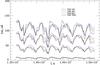 |
Fig. 9 As Fig. 8 but for lines of Fe ii λ5500 Å with Ei = 1,3,5,10 eV. |
| In the text | |
|
Fig. 10 Equivalent widths as a function of time for lines of Fe i λ5500 Å with excitation energy Ei = 1,3,5 eV. The EWs are calculated by replacing the 2D hydrodynamic velocity field by an isotropic, depth-independent Gaussian microturbulent velocity of ξmic = 3 km s-1. |
| In the text | |
|
Fig. 11 Microturbulent velocity Vmic as a function of time for lines of Fe i λ5500 Å with Ei = 1,3,5 eV. log gf1 (strongest line) > log gf2> log gf3> log gf4 (weakest line). |
| In the text | |
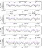 |
Fig. 12 Like Fig. 11 but for line of Fe ii λ5500 Å with Ei = 1, 3, 5, 10 eV. |
| In the text | |
|
Fig. 13 Time dependence of the non-normalized line equivalent width contribution functions of the weakest Fe i λ5500 Å Ei = 1 eV line (left panel) and the temperature profiles (right panel). The contribution functions and the temperature profiles for each instance in time are depicted in corresponding colours. |
| In the text | |
|
Fig. 14 Fe iEi = 1 eV and Fe ii Ei = 1 eV line profiles for the strongest case as a function of photometric phase. Photometric phase φp zero coincides with maximum light. |
| In the text | |
|
Fig. 15 Line asymmetries of the Fe i λ5500 Å with Ei = 3 eV as a function of the dynamical phase φd. Line strength changes in order of oscillator strength with log gf1> log gf2> log gf3 > log gf4. Dynamical phase zero coincides with the velocity reversal from contraction to expansion in the photosphere. The line asymmetry curves are shifted by 0.5 dex relative to each other for clarity. |
| In the text | |
|
Fig. 16 Effective temperature as function of the Fe i λ6085.27 Å and Si i λ6155.14 Å line depth ratio for two different abundances. Big circles connected by a blue line mark a case with + 0.4 dex abundance increase for Si and Fe; small circles connected by a red line mark a case with −0.4 dex. The colour of the circles indicates the photometric phase φp. The dashed curve depicts the calibration of Kovtyukh (2007) for supergiants. |
| In the text | |
|
Fig. 17 The line profiles of Fe i 1 Ei = 1 eV for two extreme cases (black) of the minimum (blue) and maximum (red) of the spectroscopic radial velocity and measured Doppler shifts of the the line-core position by using a parabolic fit to the core region, by using a Gaussian fit to the whole profile and the centroid velocity. |
| In the text | |
|
Fig. 18 Radial velocities as a function of time obtained by measuring the Doppler shift of Fe i λ5500 Å Ei = 1 eV (blue), 3 eV (red), 5 eV (green) line cores using parabolic fits. Four different line strengths are shown whose EWs are ordered according to their oscillator strength log gf1 > log gf2 > log gf3 > log gf4. The velocity curves are shifted by 40 km s-1 relative to each other for clarity. |
| In the text | |
|
Fig. 19 Time-averaged radial velocities ⟨v⟩t of Fe i and Fe ii lines as a function of their EW. The measurement of the Doppler shift is based on parabolic fits of the line core deeper than 70% of the total line depth. |
| In the text | |
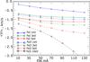 |
Fig. 20 Like Fig. 19, but measuring the Doppler shift by a Gaussian fit of the whole line profile. |
| In the text | |
|
Fig. 21 Time-averaged radial velocities ⟨v⟩t of Fe i and Fe ii lines as a function of their EW. The measurement of the Doppler shift is based on the barycenter of the spectral line. |
| In the text | |
|
Fig. 22 Time-averaged radial velocities from line core fitting when pulsations have not set in. |
| In the text | |
|
Fig. 23 Time-averaged radial velocities from Gaussian fitting when pulsations have not set in. |
| In the text | |
|
Fig. 24 Time-averaged barycenter radial velocities when pulsations have not set in. |
| In the text | |
|
Fig. 25 Pulsational velocity as a function of the radial velocity, estimated by Gaussian fits of the whole Fe i Ei = 1 eV line profiles. Colours show different line strengths: the strongest line is depicted in black, the weakest in blue. The slope of the linear regression is the p-factor. |
| In the text | |
|
Fig. 26 Residual velocity or K-term derived by linear fits of the curve vpuls = p × vrad + vo and K = −vo/p for different line strengths and excitation potentials. The spectroscopic radial velocity is measured by Gaussian fitting. |
| In the text | |
|
Fig. 27 Vertical geometric coordinate of a layer in the photosphere with τR = 2/3, and the corresponding pseudo-Lagrangian mass element as a function of time. |
| In the text | |
|
Fig. 28 Pulsational velocities of a layer in the photosphere with τR = 2/3, and of the corresponding pseudo-Lagrangian mass element as a function of time. |
| In the text | |
Current usage metrics show cumulative count of Article Views (full-text article views including HTML views, PDF and ePub downloads, according to the available data) and Abstracts Views on Vision4Press platform.
Data correspond to usage on the plateform after 2015. The current usage metrics is available 48-96 hours after online publication and is updated daily on week days.
Initial download of the metrics may take a while.