| Issue |
A&A
Volume 606, October 2017
|
|
|---|---|---|
| Article Number | A30 | |
| Number of page(s) | 13 | |
| Section | The Sun | |
| DOI | https://doi.org/10.1051/0004-6361/201730839 | |
| Published online | 03 October 2017 | |
Reconstruction of a helical prominence in 3D from IRIS spectra and images⋆
1 LESIA, Observatoire de Paris, PSL Research University, CNRS, Sorbonne Universités, UPMC Univ. Paris 06, Univ. Paris-Diderot, Sorbonne Paris Cité, 5 place Jules Janssen, 92195 Meudon, France
e-mail: This email address is being protected from spambots. You need JavaScript enabled to view it.
2 Astronomical Institute, Academy of Sciences of the Czech Republic, Fričova 298, 25165 Ondřejov, Czech Republic
e-mail: This email address is being protected from spambots. You need JavaScript enabled to view it.
3 Institut de Recherche en Astrophysique et Planétologie, 31028 Toulouse, France
4 SUPA School of Physics and Astronomy, University of Glasgow, Glasgow, G12 8QQ, UK
5 Université de Orléans, 45100 Orléans, France
Received: 21 March 2017
Accepted: 14 June 2017
Abstract
Context. Movies of prominences obtained by space instruments e.g. the Solar Optical Telescope (SOT) aboard the Hinode satellite and the Interface Region Imaging Spectrograph (IRIS) with high temporal and spatial resolution revealed the tremendous dynamical nature of prominences. Knots of plasma belonging to prominences appear to travel along both vertical and horizontal thread-like loops, with highly dynamical nature.
Aims. The aim of the paper is to reconstruct the 3D shape of a helical prominence observed over two and a half hours by IRIS.
Methods. From the IRIS Mg ii k spectra we compute Doppler shifts of the plasma inside the prominence and from the slit-jaw images (SJI) we derive the transverse field in the plane of the sky. Finally we obtain the velocity vector field of the knots in 3D.
Results.We reconstruct the real trajectories of nine knots travelling along ellipses.
Conclusions. The spiral-like structure of the prominence observed in the plane of the sky is mainly due to the projection effect of long arches of threads (up to 8 × 10⁴ km). Knots run along more or less horizontal threads with velocities reaching 65 km s-1. The dominant driving force is the gas pressure.
Key words: Sun: filaments, prominences / Sun: UV radiation / Sun: magnetic fields
Movies associated to Figs. 1, 9, 10, and 13 are available at http://www.aanda.org
© ESO, 2017
1. Introduction
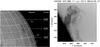 |
Fig. 1 Left panel: filament observed with the Meudon spectroheliograph in Hα on July 15, 2014 at 07:20 UT. Right panel: the corresponding filament (in reverse colour) as it crossed the limb as a prominence on July 17, 2014, observed by SOT using the Ca ii filter at 08:04 UT. A movie of the SOT image is available online (Movie 1). |
The Solar Optical Telescope (SOT; Tsuneta et al. 2008; Suematsu et al. 2008) aboard the Hinode satellite (Kosugi et al. 2007) has observed prominences in Hα and the chromospheric Ca ii lines. It revealed the highly dynamical nature of cool plasma in prominences (Labrosse et al. 2010; Dudík et al. 2012). The Solar Dynamics Observatory spacecraft and its high spatial and temporal resolution imager, the Atmospheric Imaging Assembly (SDO, AIA; Lemen et al. 2012) allow us to follow the dynamics of prominences or filamenst when observed on the disk in transition-region and coronal filters (304 Å filter ~105 K, 171 Å and 193 Å filters ~106 K; Parenti et al. 2012).
AIA movies reveal that some prominence structures when arriving close to the limb look like tornadoes, with an apparent rotation motion around their vertical axis (Su et al. 2012, 2014; Li et al. 2012; Panesar et al. 2013; Levens et al. 2015). The Extreme-ultraviolet Imaging Spectrometer (EIS; Culhane et al. 2007) on board Hinode has provided spectral scans covering prominence-tornado structures in different wavelengths (170–211 Å and 246–292 Å). The Dopplergrams of such structures presented blueshifts on one side of the vertical structure and redshifts on the other side (Su et al. 2014; Levens et al. 2015). These former authors used time-distance diagrams from coronal filtergrams taken with the AIA to quantify sinusoidal oscillations in tornadoes, finding periods of about one hour and apparent rotational velocities of 6–8 km s-1. A sit-and-stare EIS run showed that this kind of pattern could survive for three hours suggesting a long life of the rotation motion (Su et al. 2014).
These observations in hot lines (>106 K) concern mainly the interface of cool prominences (104 K) with the corona. It appears important to understand the dynamics of the cool plasma inside these structures. Attempts have been made to derive the line-of-sight velocity of the cool plasma using chromospheric lines observed by ground-based telescopes. Swirling motions in the low atmosphere were detected using the Crisp Imaging Spectropolarimeter at the Swedish Solar Telescope (CRISP, SST; Scharmer et al. 2003; Wedemeyer & Steiner 2014). However they do not appear to be related to filamentary structures. On the other hand, high dark vertical structures observed at the limb with the CRISP, which look like tornadoes in AIA filters, have been interpreted as legs of prominences (Wedemeyer et al. 2013). Prominence tornadoes have been observed in the He i 10 830 Å line with the Tenerife Infrared Polarimeter at the Vacuum Tower Telescope in Tenerife (TIP, VTT; Orozco Suárez et al. 2012; Martínez González et al. 2016). Both sit-and-stare observations along a slit and scans of a region with a cadence of half an hour have been performed. Using the sit and stare mode, Orozco Suárez et al. (2012) found an anti-symmetric Doppler curve similar to the result found by Su et al. (2012) using EIS. Martínez González et al. (2016) used the scanning mode and obtained four consecutive spectro-polarimetric scans in four hours. The latter authors could not find any coherent behaviour between the two scans and concluded that, if rotation exists, it must be intermittent and last less than one hour. In fact, the incoherence that they found has been explained by observations of a tornado made using the Meudon Solar Tower and the Multi Subtractive Double Pass (MSDP) spectrograph, which provides Dopplergrams with a cadence of 30 s. Over a period of two hours large cells of blueshifts and redshifts have been observed in a prominence (Schmieder et al. 2017). Over a period of 30 min it was found that redshifted cells became blueshifted, and vice versa. They explained this quasi-periodicity in the Doppler shift maps as being caused by oscillations of the dipped magnetic structure sustaining the prominence plasma, and not by rotation of the structure. In prominences the magnetic field is parallel to the photosphere, with cool plasma suspended in dips (Aulanier & Démoulin 1998; López Ariste et al. 2006; Dudík et al. 2008; Gunár & Mackay 2015, 2016). Vector magnetograms have been obtained using the polarimeter at the Télescope Héliographique pour l’Étude du Magnétisme et des Instabilités Solaires (THEMIS, French telescope in the Canary Islands-see López Ariste et al. 2000; Bommier et al. 2005), and they confirmed that the magnetic field in tornado-like prominences is roughly horizontal (Schmieder et al. 2014; Levens et al. 2016a; 2016b, and in prep.). Helical motions have been detected in prominences (Martínez González et al. 2015; Zapiór & Martínez-Gómez 2016). For example, knot trajectories along elliptical loops have been computed using a method of 3D reconstruction developed in Zapiór & Rudawy (2012). We shall use the same method in the present paper. Such a kind of helical structure could correspond to the theoretical model of a tornado (Luna et al. 2015).
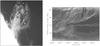 |
Fig. 2 Left panel: prominence observed by SOT using the Ca ii K filter at 08:10 UT on July 17. Crosses follow an elliptical loop from right (A) to left (B). Right panel: time-distance diagram for the path along the loop joining A and B. The black vertical lines in the diagram are missing data. |
During a coordinated campaign in July 2014, many prominences were observed using the SOT instrument aboard Hinode, and the Interface Region Imaging Spectrograph (IRIS; De Pontieu et al. 2014). We focus this study on a prominence observed on July 17, 2014, with an apparent helical structure (Sect. 2). A few days before, this structure was a north-south oriented filament, with some extent in the east-west direction (Fig. 1). The IRIS and SOT fields of view were centred on a section of the filament as it crossed the limb (Sect. 2). The prominence has an anti-symmetric Doppler pattern in the Mg ii k line observed with the IRIS spectrograph (Sect. 3). The reconstruction of the vector velocity field in 3D is possible by combining high spatial and temporal resolution IRIS SJI images in Mg ii k and IRIS spectra.With the 3D reconstruction we demonstrate that the apparently helical prominence consists of a horizontal magnetic structure with no real twist (Sect. 4).
2. Observation of a helical prominence
2.1. IRIS
IRIS performed a 16-step coarse raster observation from 08:40:07 UT to 12:01:44 UT on July 17, 2014. The pointing of the telescope was (850′′, 454′′), with a spatial pixel size of 0.167′′. The raster cadence of the spectral observation in both the near ultraviolet (NUV, 2783 to 2834 Å) and far ultraviolet (FUV, 1332–1348 Å and 1390–1406 Å) wavelength bands was 86 s. Exposure time was 5.4 s per slit position. 140 scan images, each covering 30′′ × 119′′, can be reconstructed using the 16 spectra obtained during the raster process of the region with a step of 2′′. Slit-jaw images (SJI) in the broad band filters (2796 Å and 1330 Å) were taken simultaneously with a cadence of 11 s. The filed of view (FOV) of the SJI was 119′′ × 119′′. Calibrated level 2 data are used for this analysis, with dark current subtraction, flat field correction, and geometrical correction having all been taken into account (De Pontieu et al. 2014).
We mainly use the Mg ii k 2796.35 Å line along with the slit-jaw images in the 2796 Å filter for this study. The Mg ii k line is formed at chromospheric plasma temperatures (~104 K). The SJI 2796 Å filter is dominated by emission from the Mg ii k line. The co-alignment between the optical channels is achieved by comparing the positions of horizontal fiducial lines.
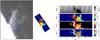 |
Fig. 3 Prominence observed on July 17, 2014 by SOT in Ca II at 09:02 UT and its magnetic field strength from THEMIS at 09:29 UT overlaid by a box, which represents the field of view of THEMIS observations presented in the right panels: (from top to bottom) intensity in the He i D3 line, magnetic field strength, magnetic field inclination with respect to the local vertical and magnetic field azimuth with respect to the line of sight. In the rotation of the field of view of THEMIS, the limb is along the x-axis. |
2.2. Hinode/SOT
The Hinode/SOT telescope consists of a 50 cm diffraction-limited Gregorian telescope and a Focal Plane Package including the narrowband filtergraph (NFI), broadband filtergraph (BFI), the Stokes Spectro-Polarimeter, and Correlation Tracker (CT). For this study, images were taken with a 16 s cadence in the Ca ii H line at 3968.5 Å using the BFI with a 3 Å bandpass between 08:04:30 UT and 09:02:54 UT. The Ca ii images have a pixel size of 0.109′′ and an exposure time of 1.22 s, with a field of view of 112′′ × 112′′.
Figure 1 (right panel) and the Movie 1 (animated movie of Fig. 1) show the helical structure of the prominence observed with SOT. The observing times of IRIS and SOT overlap for only 20 min. The spatial scale of SOT (0.109′′) is better than that of the IRIS SJI (0.167″ × 0.167′′), therefore very fine structures are resolved.In the SOT movie we see some small fragments of the prominence, that we will call “knots”, moving up and down along expanding, and then contracting, helical structures over the course of an hour.At the beginning of Movie 1, the helical structure rises, reaches the top of the field of view, and progressively the height of the loops is reduced. This is visible if we compare the three images of SOT at three different times within the same field of view in Figs. 1–3.
Figure 2(right panel) shows the time distance diagram obtained along a path following one ellipse of the helical structure from its right leg to its left leg after having co-aligned all the frames of SOT. The right leg (between 0′′ and 20′′) is moving toward the right and the motions of the knots cannot be seen because they are going out of the path, but the knots along the right leg (between 40′′ and 90′′) show transverse velocities from 10 km s-1 to 70 km s-1. They are all descending in the same direction indicating the existence of many parallel threads.
2.3. THEMIS spectropolarimetry
For several campaigns, the French telescope Télescope Héliographique pour l’Étude du Magnétisme et des Instabilités Solaires (THEMIS) in the Canary Islands (López Ariste et al. 2000) with the MulTi-Raies (MTR) mode has adopted an almost fixed setup for the observation and measurement of magnetic fields in prominences. The large collection of prominences observed has resulted in several publications (Schmieder et al. 2013, 2014; Levens et al. 2016a). In the observations used in the present work, the slit of the MTR spectrograph, oriented parallel to the limb, was scanning mainly the base of the prominence (see the blue box in Fig. 3 left panel). The observations consist of three successive rasters of 20 positions with 2′′ between slit positionsstarting at 09:29 UT, 10:26 UT, and 11:20 UT. The pixel size along the slit was of 0.2′′, but seeing conditions and the long exposure times required for polarimetry reduce the resolution to around 1′′.
The acquisition of a full raster takes less than one hour. THEMIS polarization analysis is based on a beamsplitter polarimeter. A grid-like mask is used to split the field of view and leave place, at intervals of 15.5 arcsec, for the secondary beam originating in the polarimeter beamsplitter (more details available in Schmieder et al. 2013). The images are obtained by two successive displacements of the grid along the slit to cover the full spectra of the four Stokes parameters (I, Q, U, and V) in the doublet of the He i D3 5876 Å line. This is the reason behind the light grey vertical bars in the images. The bars are not rectangular due to some shift in the instrument during the observation (Fig. 3 top left panel).
As in previously cited studies of prominences using this setup, raw data was reduced using the DeepStokes procedure (López Ariste et al. 2009) and the resulting Stokes profiles were fed to an inversion code based on Principal Component Analysis and able to identify both the Zeeman and Hanle effects in the Stokes profiles (López Ariste & Casini 2002; Casini et al. 2003). These codes rely on a database of pre-computed profiles (around 90 000 for the database used here) among which the solution is found. The database is dense enough for the solution to fit the observations up to noise levels if the observed profile can be explained by a single vector magnetic field per pixel in the absence of radiative transfer. Error bars for each of the physical parameters retrieved are determined by performing statistics on all other models which are similar to the observed profile, but not as similar as that which is selected as the solution. Errors can have two meanings: random errors are due to the combined effect of noise in the data and the coarseness of the database. They are acceptably small. For example, random errors in the inclination of the magnetic field are known to be on the order of 10°. Larger errors are the result of either ambiguities (for example the 180° ambiguity in the azimuth of the field) or, more often, are caused by observed profiles that cannot be explained by the simple model of a single vector field per pixel.
Figure 3 (right panels) presents the maps obtained after the inversion of the Stokes parameters recorded in the He i D3 line(from top to bottom): intensity, magnetic field strength, inclinationwith respect to the local vertical, and azimuth with respect to the line of sight. The origin angle of inclination is the local vertical and the origin of the azimuth is the line of sight (LOS) in a plane containing the LOS and the local vertical. We see that the brightest parts of the prominence have a mean inclination of 90°, which means that the magnetic field in these parts is horizontal. However, there is a large dispersion of the values (±30°) from one pixel to the next in the prominence. The 60° inclination pixels are mainly in the centre of the prominence between the two different legs.
The histogram of the inclination for all the points in the prominence shows that the quality of the inversion is not as good as for former prominences (Levens et al. 2016b). There are only a few points in the peak, centred on 90°, indicating an horizontal direction (Fig. 4). Those results have small error bars of less than 10° which, as said above, correspond to random errors mostly due to noise in the data. We are confident that these horizontal magnetic fields in the prominence are correctly measured.Most of the points belong to two secondary peaks at around 50° and 120°, but they show large error bars (>30°). A few points around 55° have an error bar less than 10°. A first conclusion would be that the inclination is 60 or 110 degrees and the Principal Component Analysis (PCA) inversor code cannot decide what the best solution is because of the 90° ambiguity. However, in another prominence observed by IRIS where the histograms showed similar distributions of values, Schmieder et al. (2014) related this distribution to the fact that the prominence was very dynamic. A numerical test confirmed that when the polarized profiles were due to the addition of an horizontal field plus a turbulent field, the resulting profile would yield 60–110 solution with 30° errors. Since this paper, many prominences (López Ariste 2015) have shown similar histograms and we propose the same interpretation for the present case with the superposition of two magnetic fields inside the pixel: an horizontal background field set inside a turbulent ambient field. We note that these pixels with large errors are mainly between the two legs of the elliptical loops where no structures could really be resolved.
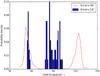 |
Fig. 4 Histogram of the magnetic field inclination with respect to the line of sight measured in the prominence on July 17, 2014. |
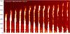 |
Fig. 5 IRIS Mg ii k spectra during the first scan between 08:40:07 and 08:41:28 UT. Only the spectra crossing the prominence are shown (3 to 16). The left column represents the number of the pixels along the slit with a unit equal to the pixel size (0.167′′). The number of each position of the slit is indicated in the spectra at the bottom of the image. |
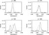 |
Fig. 6 Examples of Mg ii k line profiles along slit 13 at 08:41:12 UT during the first scan of the tornado. The dashed profile is a mean profile, averaged along the slit. The graph titles represent the position of the pixel along the slit (see Fig. 5). The intensity unit is in erg s-1 sr-1 m-2 Hz-1. |
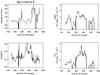 |
Fig. 7 Doppler shift, peak intensity, total intensity, and FHMW of the Mg ii k profiles along slit 13 at 08:41:12 UT during the first scan of the tornado. |
3. Spectral analysis of IRIS
3.1. Doppler shifts
Figure 5 shows an example of a set of Mg ii k spectra obtained during the first raster. The left column indicates the pixel number along the slit. We note the presence of reversed profiles on the disk. Spectra 3 to 6 show a dense part of the prominence, while spectra 7 to 16 show a less dense part where elliptical loops can be distinguished. The profiles of the Mg ii k line spectra from the helical part of the prominence are mainly non-reversed. The spectra in the upper part are very shifted indicating high Doppler shifts. Examples of profiles are shown in Fig. 6. The reference profile in these plots is a mean profile obtained by averaging the profiles of pixels above the limb along one slit.We note that there are a number of different profiles in this prominence: some profiles are narrow (y = 390), some profiles are reversed (y = 470), some profiles have double components (y = 550), indicating the presence of two or more structures along the line of sight, and in some locations the entire profile is Doppler shifted (y = 590).
Different methods have been tested to compute the Doppler shifts. In a first attempt, the profilesare fitted using Gaussian functions which are then used to derive the main characteristics of the prominence plasma. The Full Width at Half Maximum (FWHM) is around 0.2 Å and the profiles are commonly narrow in prominences, as was the case in Schmieder et al. (2014). However, there are exceptions where the FHMW reaches 0.4 or 0.6 Å. In these cases it appears that the profiles are certainly a combination of different structures along the LOS with different velocities. Assuming Gaussian profiles for the IRIS Mg ii lines, we return relatively small line-of-sight velocities (±5 km s-1) for wide profiles. For narrow profiles, higher Doppler shifts are measured, reaching 60 km s-1. These points correspond to the highest points along the slit and more or less the top of the prominence (e.g. profile at y = 590 in Fig. 6). Such points belong to the knots that have been followed along the elliptical structures (see Sect. 4).
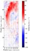 |
Fig. 8 Doppler shift map of the prominence observed on July 17, 2014 between 08:40:07 and 08:41:34 UT with IRIS. The Doppler shifts have been computed from the gravity centre of the Mg ii k line profiles. The pixel size in the y direction has been degraded to 2′′ to have a square pixel.The colour bar shows Doppler shift in km s-1.The dashed line approximately indicates the limb. |
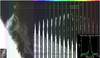 |
Fig. 9 Slit-jaw image and corresponding spectra taken during one scan between 10:15:10 and 10:16:29 UT (animated image is online, see Movie 2). Dotted vertical lines indicate slit position in the FOV. Corresponding spectra are colour coded. White rectangle on the slit-jaw image shows knot area, which is magnified in the bottom-left corner. Red lines show 99% isophote. White rectangle on the spectra (top-right) indicates area of the spectrum which is taken for further analysis. |
3.2. Doppler pattern
We analyse the Mg ii spectra of the first raster, beginning at 08:40:07 UT and ending at 08:41:24 UT, along the 16 slit positions. As some profiles are reversed (either due to absorption or to the presence of different structures along the line of sight) it is more useful to compute Doppler shifts by using the gravity centre of each profile than to fit the profile with a Gaussian curve. The spatial resolution is degraded in the y direction to 2′′, which corresponds to the step size in x. We obtain the Doppler pattern of the prominence (Fig. 8). The resulting Doppler map shows an anti symmetric pattern with strong redshift in the left part of the prominence and blue shift in the right part, similar to those patterns found with the spectroscopic data of EIS in Fe xii at 195 Å. These patterns could suggest the existence of rotation around the axis of the prominence, an observational known as a “tornado”.
4. 3D trajectory reconstruction
The SOT movie (Movie 1 and Fig. 1 ) and the IRIS SJI movie (Movie 2 and Fig. 9) show knots following elliptical trajectories (helical shape is 3D, SOT movie and IRIS SJ are 2D, so shape in the movies should be 2D) in the plane of the sky. Even though the IRIS movie has a slightly lower spatial resolution, it has been possible to follow manually a few of the knots using the IRIS 2976 Å SJI along with the simultaneous Mg ii k spectra. In the set of slit-jaw images, we detected several prominence knots. Knots are fragments of prominence plasma, which are detached from the main prominence and move independently along magnetic field lines. They are approximately 103–104 km in diameter and usually circular or elliptic in shape.
Using the 3D trajectory reconstruction method described in Zapiór & Rudawy (2012), the positions of 15 knots in x and yare computed by polynomial approximations. Only nine knots are shown in the bottom right panel of Fig. 10 for clarity. Having analytical expressions for x(t) and y(t), projections of velocity vectors vx(t) and vy(t) are calculated as derivatives of x(t) and y(t). The Doppler shifts of the IRIS spectra give the third component along the z axis, which is oriented awayfrom the plane of the sky, x and y being in the plane of the sky (plane of the images). The reference system used here is not the conventional one. The y-axis makes an angle of 60° with the radial direction and an angle of 10° with the main direction of the prominence body, which is inclined towards the solar surface. Having the set of slit-jaw images together with the spectra, at least in the part of the prominence image, it is possible to reconstruct true 3D trajectories of knots.
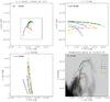 |
Fig. 10 Projections of knot trajectories onto perpendicular planes. Arrows give trajectories of particular knots together with projected velocity vector. Axes are oriented as follows: x axis oriented right in the POS along bottom edge of the slit-jaw image, y axis oriented up along left edge of the slit-jaw image, z axis oriented along LOS away from the observer. Bottom right panel shows an overplot of the vectors onto a prominence image from 10:49:44 UT (Movie 4 shows an animation of this). Thread numbers correspond to numbers in Table 1. In the ıtop left corner of each panel, reference velocity vector in the plot scale is drawn. Small rectangle in top left panel shows the area of bottom right panel, which has a different scale than the other panels. |
From the set of observations we make a “sandwich” median image from slit-jaw images of a particular scan. In other words, we stack data cubes, which consist of eight slit-jaw images per cube, and we constructedthe median image, which has a median value for each pixel. This gives a better signal-to-noise (S/N) ratio and even faint knots become visible. One scan lasts about 86 s. Over this period, the shift of an individual knot is not substantial. However, spectra were taken 2 times as frequently (i.e. 16 spectral observations during one scan). We present slit positions in an exemplary slit-jaw image in Fig. 9.
In the set of consecutive slit-jaw images, we select knots visible in at least several consecutive images. We manually select an area with a knot in the slit-jaw images (white rectangle in Fig. 9) and we identify knots as regions with signal above 99% of the brightest pixel inside the area, marked with a red isophote (see left bottom corner of Fig. 9). From the centre of gravity of the signal inside the isophote, we calculate the position of the analysed knot (xn,yn) in the plane-of-sky (POS), where n is the scan number, counted from the beginning of the observation of a particular knot.
Then, we take the spectrum corresponding to the nearest slit position (see colour coding in Fig. 9). If the selected knot area crosses more than one slit position, we calculate the spectrum as a weighted mean from the corresponding slit positions. We project the region limited by the isophote onto the vertical axis and make a sum of the signal in each row. We construct a vector of accumulated signal from each row in this way. We take into account only pixels from inside the isophote. We normalise the vector, which is then treated as a weight, Wj, where j is a row number. Next we calculate the mean weighted spectrum, S(λ), given by: 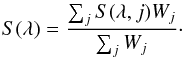 This is then treated as a knot spectrum at a particular time tn.
Foreach knot spectrum at a given time (tn) we fit a single Gaussian curve using a robust, non-linear least squares curve fitting code by Markwardt (2009), which is based on the algorithm by Moré (1978, see Fig. 11). The reason for using a single Gaussian is because knots are separate structures visible against the background dark sky. They usually have a small optical thickness. This leads to a single Gaussian profile because there is no other structure along line-of-sight (LOS). For a limited number of spectra (~25%), we find centrally reversal profiles due to the larger optical thickness. In such cases weremove the central reversal using an automated procedure. The procedure searches for points in the spectrum with lower signal between the two peaks (see Fig. 11, right panel) and removes them from the Gaussian fit. Gaussianfitting is therefore performed on spectral wings only. Fromthe shift of these Gaussians we calculate the Doppler velocity. For each scan we calculate the mean profile of the quiet photosphere and corresponding residual velocity (see Fig. 12). Residual velocity, which is caused by the orbital period of the IRIS satellite, is approximated by a cosine curve and is treated as the zero point for correction of Doppler velocity.
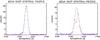 |
Fig. 11 Left panel: observed spectral profile (blue points) of an analysed knot with regular Gaussian shape. Right panel: spectral profile of an analysed knot with central reversal (red points). Gaussian fitting is performed on blue points only. Black dashed lines show fitted Gaussian profile. |
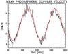 |
Fig. 12 Mean photospheric Doppler velocity calculated from the quiet photosphere, which is treated as the zero velocity level. |
For each knot we have a set of data: tn – time of observation taken as a time of the first spectrum in a scan, x(tn),y(tn) – POS position of a knot, vD(tn) – Doppler velocity, where n = 1,...,N and N is a total number of observations of a particular knot. We then perform an approximation of x(tn),y(tn),vD(tn) using polynomials. To find a polynomial that properly describes the observed variations, we make use of orthogonal Chebyshev polynomials of the first kind, Tm(t). We successively perform an approximation of the data points x(tn),y(tn),vD(tn)using LSE method with a sum of Chebyshev polynomials with coefficients am as free parameters with consecutively higher orders:  where Pm = fitting polynomial of the data points, Tm = Chebyshev polynomial of the m degree.
We calculate the t-Student statistic  for m = 0, 1,...,10. Calculation of this statistic for higher m values was unnecessary because knot trajectories are well described by polynomials of low degrees (Larmore 1953; Rothschild et al. 1955). In our case the maximum polynomial degree used for data point approximation was equal to two (see Table 1). Calculated values of Sm are compared with the critical value of the statistic t(α,M), where M = N − m − 1, M – degrees of freedom, N – number of data points, and α = 0.05 – selected significance level. We select the fitting polynomial degree as the highest m for which Sm>t(α,M) occurs. Having established degree, we can then perform fitting again with the degree equal to m, obtaining a polynomial with the correct degree. Rapid changes of the measured LOS velocity were caused by the noise, not by physical changes of the velocity related to the trajectory (see Fig. 14). This was caused by the fact that slit positions during scanning were separated. We could not have continuous measurements of the LOS along the trajectory, but only in the slit positions. We decided to approximate LOS data with low degree polynomials in order to avoid over-fitting of the data points.
Basic informationabout observed knots.
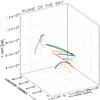 |
Fig. 13 Reconstructed 3D knot trajectories in the x, y, and z system (animated cube in Movie 3). X and y are in the plane of the sky, z is oriented along the LOS away from the observer. Thin lines are projections onto plane of the sky (x,y). Colours correspond to the colours used in the plots in Fig. 10. |
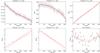 |
Fig. 14 Kinematic properties of knot number 7. Black points with error bars represent data points xn,yn,vn. Red solid lines represent polynomial fits, their derivatives (for vx and vy), and integral (for Δz). Dashed lines represent fitting errors estimated using bootstrap resampling (see e.g. Andrae 2010). |
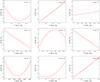 |
Fig. 15 Spatial velocity (in km s-1) of all observed knots in the space versus time. The horizontal axes are scaled in seconds from the first time of observation of each knot (t1 – see Table 1). Dashed lines give error estimations from bootstrap resampling method. |
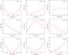 |
Fig. 16 Curvature radius (in units of 103 km) of all observed knots. The horizontal axes are scaled in seconds from the first time of observation of each knot (t1 – see Table 1). Dashed lines give error estimations from bootstrap resampling method. |
As a result ofthe approximation, we have a continuous variation of x(t),y(t), and vD(t). We then integrate vD(t) and obtain Δz(t) – the relative shift along the LOS. Having x(t),y(t), and Δz(t) (see Fig. 14), we have a complete spatial 3D trajectory for each knot. We need to stress here that unless the initial position of the calculated trajectory is not known, values x(t),y(t),Δz(t) represent its true 3D geometry. We can arbitrarily shift each knot’s trajectory along the z axis, but the 3D shape is conserved (Fig. 13 and Movie 3). We assume that z(t1) = 0. Having analytical variations of x(t), y(t), and vD(t), calculation of projections of velocity onto perpendicular axes (vx,vy,vz), perpendicular planes (vxy,vyz,vxz), spatial velocity (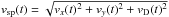 ), and local curvature radius (rc = vsp(t)2/an(t), where an(t) – acceleration normal to instantaneous velocity vector) is possible (Figs. 10, 15, 16, and Table 1).
All knots have similar kinematic properties. They follow parallel directions with similar curvature radii (Fig. 16). The curvature is calculated locally according to the position of Frenet-Serret formulas, that is, the curvature radius is local in the direction perpendicular to local velocity in the plane of local surface in which the motion occurs. Knots seem to have motions in the plane with no pitch (twist). No helical motions are observed. 3D trajectories of knots are nearly plane curves. Discrepancies of the velocity behaviour are present because knots are observed in different parts of the prominence body (Fig. 15). Also we do not know the relative position of knot trajectories along LOS, so knots observed close to each other in the POS may be more separated than they seem.
However, we notice some similarity in the behaviour of thevariation of the velocity norm of a pair of knots: knots 2 and 9 have an increasing velocity, knots 4 and 6 a decreasing velocity. Knots 1 and 7, which are observed for more than 30 min, first have a decreasing velocity norm then an increasing velocity norm. Knots 2 and 9 are on parallel trajectories going upwards, knots 4 and 6 are on parallel trajectories going downwards. Their acceleration behaviour is contrary to thegravitational force. We conclude that the knots are moving due to gas pressure andnot due to gravity.
5. Discussions and conclusions
During a coordinated campaign with space instruments IRIS and Hinode/SOT and the vector magnetograph THEMIS in the Canary Islands, a prominence was observed on July 17 2014. This prominence is a north-south oriented filament but which is east-west extended, crossing the limb. The prominence appears to have a helical shape, with plasma turning along elliptical paths(as seen in Movies 1 and 2). We computed Doppler shifts by taking the gravity centre of the IRIS Mg ii k line profiles, and we obtained an anti-symmetric pattern with strong redshifts around the axis of the prominence, suggesting a rotational motion around the axis, much like that seen in AIA “tornadoes” (Su et al. 2014; Levens et al. 2015).The spatial scale has been degraded to 2′′ in order to have square pixels, and this explains why we do not see the Doppler shift of each individual knot.
A 3D reconstruction technique (Zapiór & Rudawy 2012) combining the IRIS slit jaw images and the high resolution spectra of IRIS in the Mg ii k line allowed us to compute the velocity vector field in the volume of the prominence. The transverse velocity measured by using the SJI of IRIS is one order of magnitude less than the Doppler shifts. The apparent helical motion of the knots along the ellipses is very slow compared to the fast speed of the knots travelling along more or less horizontal threads with velocities of up to 65 km s-1 away from the observer. The threads extended up to 80 000 km, more or less parallel to the solar surface, and not along meridians in planes without any torsion.The apparent ellipse-shape structure could correspond to the curvature of the parallels of the Sun according to the value of the P angle in July (Fig. 1 left top panel).This extension corresponds to theeast-west extent of the filament a few days before (around 5° in Fig. 1). Thedominant force which is moving the knots is found to be gas pressure and not gravity.
Using 3D reconstruction, we have demonstrated that this prominence is a typical prominence and does not have the characteristics of a tornado as we thought it did at the beginning of the study. The high cadence of the movies can give false impressions of the dynamics of these structures when projected onto the plane of the sky. We need to have simultaneous spectra and images to correctly interpret the movies.
The horizontality of the threads forming the prominence is consistent with the inclination of 90° found with THEMIS (Fig. 4). Combining data from two instruments with different spatial resolution and different cadence is difficult and can lead to confusion when interpreting the observations. However, THEMIS is one of the few instruments able to measure magnetic fields in prominences, together with the TIP instrument of the VTT. Such measurements come at a price: spatial and temporal resolutions are poor. Such information must always come from other instruments, SOT and IRIS in the present work. It would be certainly better to measure magnetic fields while maintaining an acceptable time cadence and a nice spatial resolution. A combination of adaptive optics, spectro-imagery and polarimetry would be desirable, if possible, in several spectral domains.
We have also to note that the polarization is measured in different lines from the chromospheric lines in which prominences are observed. These lines have different characteristics (temperature, optical thickness) and they certainly formed in different structures. These theoretical problems should be resolved by non local thermodynamic equilibrium (NLTE) modelling of polarized light in the future.
Movies
Movie of Fig. 1 Access Supplementary Material
Movie of Fig. 9 Access Supplementary Material
Movie of Fig. 10 Access Supplementary Material
Movie of Fig. 13 Access Supplementary Material
Acknowledgments
The authors thank S. Gunar, B. Gelly, and the team of THEMIS for assisting with the observations. We would like to thank Jean-Marie Malherbe and Thierry Roudier whoco-aligned the SOT frames. They tested, up to now unsuccessfully, the CST and LCT methods to derive the flow pattern in the plane of the sky. We thank J. Dudik who provided the time-distance code to track the knots in the SOT cube of data, and G. Aulanier and P. Démoulin for fruitful discussions. This paper was discussed during the ISSI workshop (PI N. Labrosse) on “Solving the prominence paradox”. P.J.L. acknowledges support from an STFC Research Studentship. N.L. acknowledges support from STFC grant ST/I001808/1. Hinode is a Japanese mission developed and launched by ISAS/JAXA, with NAOJ as domestic partner and NASA and STFC (UK) as international partners. It is operated by these agencies in co-operation with ESA and NSC (Norway). IRIS is a NASA small explorer mission developed and operated by LMSAL with mission operations executed at NASA Ames Research Centre, and major contributions to downlink communications funded by the Norwegian Space Center (NSC, Norway) through an ESA PRODEX contract. The AIA data are provided courtesy of NASA/SDO and the AIA science team. M.Z. acknowledges support from the project RVO:67985815 of the Czech Academy of Sciences.
References
- Andrae, R. 2010, ArXiv e-prints [arXiv:1009.2755] [Google Scholar]
- Aulanier, G., & Démoulin, P. 1998, A&A, 329, 1125 [Google Scholar]
- Bommier, V., Rayrole, J., & Eff-Darwich, A. 2005, A&A, 435, 1115 [NASA ADS] [CrossRef] [EDP Sciences] [Google Scholar]
- Casini, R., López Ariste, A., Tomczyk, S., & Lites, B. W. 2003, ApJ, 598, L67 [NASA ADS] [CrossRef] [Google Scholar]
- Culhane, J. L., Harra, L. K., James, A. M., et al. 2007, Sol. Phys., 243, 19 [Google Scholar]
- De Pontieu, B., Title, A. M., Lemen, J. R., et al. 2014, Sol. Phys., 289, 2733 [NASA ADS] [CrossRef] [Google Scholar]
- Dudík, J., Aulanier, G., Schmieder, B., Bommier, V., & Roudier, T. 2008, Sol. Phys., 248, 29 [NASA ADS] [CrossRef] [Google Scholar]
- Dudík, J., Aulanier, G., Schmieder, B., Zapiór, M., & Heinzel, P. 2012, ApJ, 761, 9 [NASA ADS] [CrossRef] [Google Scholar]
- Gunár, S., & Mackay, D. H. 2015, ApJ, 812, 93 [NASA ADS] [CrossRef] [Google Scholar]
- Gunár, S., & Mackay, D. H. 2016, A&A, 592, A60 [NASA ADS] [CrossRef] [EDP Sciences] [Google Scholar]
- Kosugi, T., Matsuzaki, K., Sakao, T., et al. 2007, Sol. Phys., 243, 3 [Google Scholar]
- Labrosse, N., Heinzel, P., Vial, J.-C., et al. 2010, Space Sci. Rev., 151, 243 [Google Scholar]
- Larmore, L. 1953, ApJ, 118, 436 [NASA ADS] [CrossRef] [EDP Sciences] [Google Scholar]
- Lemen, J. R., Title, A. M., Akin, D. J., et al. 2012, Sol. Phys., 275, 17 [Google Scholar]
- Levens, P. J., Labrosse, N., Fletcher, L., & Schmieder, B. 2015, A&A, 582, A27 [NASA ADS] [CrossRef] [EDP Sciences] [Google Scholar]
- Levens, P. J., Schmieder, B., Labrosse, N., & López Ariste, A. 2016a, ApJ, 818, 31 [NASA ADS] [CrossRef] [Google Scholar]
- Levens, P. J., Schmieder, B., López Ariste, A., et al. 2016b, ApJ, 826, 164 [NASA ADS] [CrossRef] [Google Scholar]
- Li, X., Morgan, H., Leonard, D., & Jeska, L. 2012, ApJ, 752, L22 [NASA ADS] [CrossRef] [EDP Sciences] [Google Scholar]
- López Ariste, A. 2015, in IAU Symp., 305, eds. K. N. Nagendra, S. Bagnulo, R. Centeno, & M. Jesús Martínez González, 275 [Google Scholar]
- LópezAriste, A., & Casini, R. 2002, ApJ, 575, 529 [NASA ADS] [CrossRef] [Google Scholar]
- López Ariste, A., Rayrole, J., & Semel, M. 2000, A&AS, 142, 137 [NASA ADS] [CrossRef] [EDP Sciences] [Google Scholar]
- López Ariste, A., Aulanier, G., Schmieder, B., & SainzDalda, A. 2006, A&A, 456, 725 [NASA ADS] [CrossRef] [EDP Sciences] [Google Scholar]
- López Ariste, A., Asensio Ramos, A., Manso Sainz, R., Derouich, M., & Gelly, B. 2009, A&A, 501, 729 [NASA ADS] [CrossRef] [EDP Sciences] [Google Scholar]
- Luna, M., Moreno-Insertis, F., & Priest, E. 2015, ApJ, 808, L23 [NASA ADS] [CrossRef] [Google Scholar]
- Markwardt, C. B. 2009, ASP Conf. Ser., 411, 251 [Google Scholar]
- Martínez González, M. J., Manso Sainz, R., Asensio Ramos, A., et al. 2015, ApJ, 802, 3 [NASA ADS] [CrossRef] [Google Scholar]
- Martínez González, M. J., Asensio Ramos, A., Arregui, I., et al. 2016, ApJ, 825, 119 [NASA ADS] [CrossRef] [Google Scholar]
- Moré, J. J. 1978, The Levenberg-Marquardt algorithm: Implementation and theory, ed. G. A. Watson (Berlin, Heidelberg: Springer Berlin Heidelberg), 105 [Google Scholar]
- Orozco Suárez, D., Asensio Ramos, A., & Trujillo Bueno, J. 2012, ApJ, 761, L25 [NASA ADS] [CrossRef] [Google Scholar]
- Panesar, N. K., Innes, D. E., Tiwari, S. K., & Low, B. C. 2013, A&A, 549, A105 [NASA ADS] [CrossRef] [EDP Sciences] [Google Scholar]
- Parenti, S., Schmieder, B., Heinzel, P., & Golub, L. 2012, ApJ, 754, 66 [Google Scholar]
- Rothschild, K., Pecker, J.-C., & Roberts, W. O. 1955, ApJ, 121, 224 [NASA ADS] [CrossRef] [Google Scholar]
- Scharmer, G. B., Bjelksjo, K., Korhonen, T. K., Lindberg, B., & Petterson, B. 2003, in Innovative Telescopes and Instrumentation for Solar Astrophysics, eds. S. L. Keil, & S. V. Avakyan, SPIE Conf. Ser., 4853, 341 [Google Scholar]
- Schmieder, B., Kucera, T. A., Knizhnik, K., et al. 2013, ApJ, 777, 108 [NASA ADS] [CrossRef] [Google Scholar]
- Schmieder, B., Tian, H., Kucera, T., et al. 2014, A&A, 569, A85 [NASA ADS] [CrossRef] [EDP Sciences] [Google Scholar]
- Schmieder, B., Mein, P., Mein, N., et al. 2017, A&A, 597, A109 [NASA ADS] [CrossRef] [EDP Sciences] [Google Scholar]
- Su, Y., Wang, T., Veronig, A., Temmer, M., & Gan, W. 2012, ApJ, 756, L41 [NASA ADS] [CrossRef] [Google Scholar]
- Su, Y., Gömöry, P., Veronig, A., et al. 2014, ApJ, 785, L2 [NASA ADS] [CrossRef] [Google Scholar]
- Suematsu, Y., Tsuneta, S., Ichimoto, K., et al. 2008, Sol. Phys., 249, 197 [NASA ADS] [CrossRef] [Google Scholar]
- Tsuneta, S., Ichimoto, K., Katsukawa, Y., et al. 2008, Sol. Phys., 249, 167 [NASA ADS] [CrossRef] [Google Scholar]
- Wedemeyer, S., & Steiner, O. 2014, PASJ, 66, S10 [NASA ADS] [CrossRef] [Google Scholar]
- Wedemeyer, S., Scullion, E., Rouppe van der Voort, L., Bosnjak, A., & Antolin, P. 2013, ApJ, 774, 123 [NASA ADS] [CrossRef] [Google Scholar]
- Zapiór, M., & Martínez-Gómez, D. 2016, ApJ, 817, 123 [NASA ADS] [CrossRef] [Google Scholar]
- Zapiór, M., & Rudawy, P. 2012, Sol. Phys., 280, 445 [NASA ADS] [CrossRef] [Google Scholar]
All Tables
All Figures
|
Fig. 1 Left panel: filament observed with the Meudon spectroheliograph in Hα on July 15, 2014 at 07:20 UT. Right panel: the corresponding filament (in reverse colour) as it crossed the limb as a prominence on July 17, 2014, observed by SOT using the Ca ii filter at 08:04 UT. A movie of the SOT image is available online (Movie 1). |
| In the text | |
|
Fig. 2 Left panel: prominence observed by SOT using the Ca ii K filter at 08:10 UT on July 17. Crosses follow an elliptical loop from right (A) to left (B). Right panel: time-distance diagram for the path along the loop joining A and B. The black vertical lines in the diagram are missing data. |
| In the text | |
|
Fig. 3 Prominence observed on July 17, 2014 by SOT in Ca II at 09:02 UT and its magnetic field strength from THEMIS at 09:29 UT overlaid by a box, which represents the field of view of THEMIS observations presented in the right panels: (from top to bottom) intensity in the He i D3 line, magnetic field strength, magnetic field inclination with respect to the local vertical and magnetic field azimuth with respect to the line of sight. In the rotation of the field of view of THEMIS, the limb is along the x-axis. |
| In the text | |
|
Fig. 4 Histogram of the magnetic field inclination with respect to the line of sight measured in the prominence on July 17, 2014. |
| In the text | |
|
Fig. 5 IRIS Mg ii k spectra during the first scan between 08:40:07 and 08:41:28 UT. Only the spectra crossing the prominence are shown (3 to 16). The left column represents the number of the pixels along the slit with a unit equal to the pixel size (0.167′′). The number of each position of the slit is indicated in the spectra at the bottom of the image. |
| In the text | |
|
Fig. 6 Examples of Mg ii k line profiles along slit 13 at 08:41:12 UT during the first scan of the tornado. The dashed profile is a mean profile, averaged along the slit. The graph titles represent the position of the pixel along the slit (see Fig. 5). The intensity unit is in erg s-1 sr-1 m-2 Hz-1. |
| In the text | |
|
Fig. 7 Doppler shift, peak intensity, total intensity, and FHMW of the Mg ii k profiles along slit 13 at 08:41:12 UT during the first scan of the tornado. |
| In the text | |
|
Fig. 8 Doppler shift map of the prominence observed on July 17, 2014 between 08:40:07 and 08:41:34 UT with IRIS. The Doppler shifts have been computed from the gravity centre of the Mg ii k line profiles. The pixel size in the y direction has been degraded to 2′′ to have a square pixel.The colour bar shows Doppler shift in km s-1.The dashed line approximately indicates the limb. |
| In the text | |
|
Fig. 9 Slit-jaw image and corresponding spectra taken during one scan between 10:15:10 and 10:16:29 UT (animated image is online, see Movie 2). Dotted vertical lines indicate slit position in the FOV. Corresponding spectra are colour coded. White rectangle on the slit-jaw image shows knot area, which is magnified in the bottom-left corner. Red lines show 99% isophote. White rectangle on the spectra (top-right) indicates area of the spectrum which is taken for further analysis. |
| In the text | |
|
Fig. 10 Projections of knot trajectories onto perpendicular planes. Arrows give trajectories of particular knots together with projected velocity vector. Axes are oriented as follows: x axis oriented right in the POS along bottom edge of the slit-jaw image, y axis oriented up along left edge of the slit-jaw image, z axis oriented along LOS away from the observer. Bottom right panel shows an overplot of the vectors onto a prominence image from 10:49:44 UT (Movie 4 shows an animation of this). Thread numbers correspond to numbers in Table 1. In the ıtop left corner of each panel, reference velocity vector in the plot scale is drawn. Small rectangle in top left panel shows the area of bottom right panel, which has a different scale than the other panels. |
| In the text | |
|
Fig. 11 Left panel: observed spectral profile (blue points) of an analysed knot with regular Gaussian shape. Right panel: spectral profile of an analysed knot with central reversal (red points). Gaussian fitting is performed on blue points only. Black dashed lines show fitted Gaussian profile. |
| In the text | |
|
Fig. 12 Mean photospheric Doppler velocity calculated from the quiet photosphere, which is treated as the zero velocity level. |
| In the text | |
|
Fig. 13 Reconstructed 3D knot trajectories in the x, y, and z system (animated cube in Movie 3). X and y are in the plane of the sky, z is oriented along the LOS away from the observer. Thin lines are projections onto plane of the sky (x,y). Colours correspond to the colours used in the plots in Fig. 10. |
| In the text | |
|
Fig. 14 Kinematic properties of knot number 7. Black points with error bars represent data points xn,yn,vn. Red solid lines represent polynomial fits, their derivatives (for vx and vy), and integral (for Δz). Dashed lines represent fitting errors estimated using bootstrap resampling (see e.g. Andrae 2010). |
| In the text | |
|
Fig. 15 Spatial velocity (in km s-1) of all observed knots in the space versus time. The horizontal axes are scaled in seconds from the first time of observation of each knot (t1 – see Table 1). Dashed lines give error estimations from bootstrap resampling method. |
| In the text | |
|
Fig. 16 Curvature radius (in units of 103 km) of all observed knots. The horizontal axes are scaled in seconds from the first time of observation of each knot (t1 – see Table 1). Dashed lines give error estimations from bootstrap resampling method. |
| In the text | |
Current usage metrics show cumulative count of Article Views (full-text article views including HTML views, PDF and ePub downloads, according to the available data) and Abstracts Views on Vision4Press platform.
Data correspond to usage on the plateform after 2015. The current usage metrics is available 48-96 hours after online publication and is updated daily on week days.
Initial download of the metrics may take a while.