| Issue |
A&A
Volume 606, October 2017
|
|
|---|---|---|
| Article Number | A105 | |
| Number of page(s) | 27 | |
| Section | Atomic, molecular, and nuclear data | |
| DOI | https://doi.org/10.1051/0004-6361/201730383 | |
| Published online | 20 October 2017 | |
Stellar laboratories
IX. New Se v, Sr iv–vii, Te vi, and I vi oscillator strengths and the Se, Sr, Te, and I abundances in the hot white dwarfs G191−B2B and RE 0503−289⋆,⋆⋆,⋆⋆⋆
1 Institute for Astronomy and Astrophysics, Kepler Center for Astro and Particle Physics, Eberhard Karls University, Sand 1, 72076 Tübingen, Germany
e-mail: This email address is being protected from spambots. You need JavaScript enabled to view it.
2 Physique Atomique et Astrophysique, Université de Mons, UMONS, 7000 Mons, Belgium
3 IPNAS, Université de Liège, Sart Tilman, 4000 Liège, Belgium
4 NASA Goddard Space Flight Center, Greenbelt, MD 20771, USA
5 Astronomisches Rechen-Institut (ARI), Centre for Astronomy of Heidelberg University, Mönchhofstraße 12-14, 69120 Heidelberg, Germany
Received: 2 January 2017
Accepted: 17 June 2017
Abstract
Context. To analyze spectra of hot stars, advanced non-local thermodynamic equilibrium (NLTE) model-atmosphere techniques are mandatory. Reliable atomic data is crucial for the calculation of such model atmospheres.
Aims. We aim to calculate new Sr iv–vii oscillator strengths to identify for the first time Sr spectral lines in hot white dwarf (WD) stars and to determine the photospheric Sr abundances. To measure the abundances of Se, Te, and I in hot WDs, we aim to compute new Se v, Te vi, and I vi oscillator strengths.
Methods. To consider radiative and collisional bound-bound transitions of Se v, Sr iv - vii, Te vi, and I vi in our NLTE atmosphere models, we calculated oscillator strengths for these ions.
Results. We newly identified four Se v, 23 Sr v, 1 Te vi, and three I vi lines in the ultraviolet (UV) spectrum of RE 0503−289. We measured a photospheric Sr abundance of 6.5+ 3.8-2.4× 10⁻⁴ (mass fraction, 9500–23 800 times solar). We determined the abundances of Se (1.6+ 0.9-0.6× 10⁻³, 8000–20 000), Te (2.5+ 1.5-0.9× 10⁻⁴, 11 000–28 000), and I (1.4+ 0.8-0.5× 10⁻⁵, 2700–6700). No Se, Sr, Te, and I line was found in the UV spectra of G191−B2B and we could determine only upper abundance limits of approximately 100 times solar.
Conclusions. All identified Se v, Sr v, Te vi, and I vi lines in the UV spectrum of RE 0503−289 were simultaneously well reproduced with our newly calculated oscillator strengths.
Key words: atomic data / line: identification / stars: abundances / stars: individual: G191-B2B / stars: individual: RE 0503-289 / virtual observatory tools
Based on observations with the NASA/ESA Hubble Space Telescope, obtained at the Space Telescope Science Institute, which is operated by the Association of Universities for Research in Astronomy, Inc., under NASA contract NAS5-26666.
Based on observations made with the NASA-CNES-CSA Far Ultraviolet Spectroscopic Explorer.
Full Tables A.15 to A.21 are only available via the German Astrophysical Virtual Observatory (GAVO) service TOSS (http://dc.g-vo.org/TOSS).
© ESO, 2017
1. Introduction
Recent spectral analyses (cf., Rauch et al. 2017) of high-resolution UV spectra of the helium-rich (DO-type) white dwarf (WD) RE 0503−289 (RX J0503.9−2854, WD 0501+527, McCook & Sion 1999a,b) revealed strongly enriched trans-iron elements (atomic numbers Z ≥ 30) in its photosphere (Fig. 1). Efficient radiative levitation (Rauch et al. 2016a) in this hot WD (effective temperature Teff = 70 000 ± 2000 K, surface gravity log (g/ cm s-2) = 7.5 ± 0.1, Rauch et al. 2016b) can increase abundances by more than 4 dex compared with solar values. In the cooler (Teff = 60 000 ± 2000 K, log g = 7.6 ± 0.05, Rauch et al. 2013), hydrogen-rich (DA-type) WD G191−B2B (WD 0501+527, McCook & Sion 1999a,b), the radiative levitation is able to retain only a factor of ≈100 fewer trans-iron elements in the photosphere than in RE 0503−289 (Fig. 1).
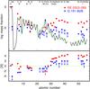 |
Fig. 1 Solar abundances (Asplund et al. 2009; Scott et al. 2015a,b; Grevesse et al. 2015, thick line; the dashed lines connect the elements with even and with odd atomic number) compared with the determined photospheric abundances of RE 0503−289 (red squares, Dreizler & Werner 1996; Rauch et al. 2012, 2014a,b, 2015, 2016a,b, 2017, and this work). The uncertainties of the WD abundances are about 0.2 dex in general. Arrows indicate upper limits. Top panel: abundances given as logarithmic mass fractions. Bottom panel: abundance ratios to respective solar values, [X] denotes log (fraction/solar fraction) of species X. The dashed, green line indicates solar abundances. |
The search for signatures of trans-iron elements in the spectra of RE 0503−289 and G191−B2B was initiated by the discovery of Ga, Ge, As, Se, Kr, Mo, Sn, Te, I, and Xe lines in RE 0503−289 (Werner et al. 2012b). Subsequent calculations of transition probabilities allowed reliable abundance determinations of Zn (atomic number Z = 30), Ga (31), Ge (32), Kr (36), Zr (40), Mo (42), Xe (54), and Ba (56) (e.g., Rauch et al. 2017, and references therein). Based on the wavelengths provided by the Atomic Spectra Database (ASD1) of the National Institute of Standards and Technology (NIST), we have identified some strong lines of strontium (38), an element that was hitherto not detected in hot WDs. For an identification of other, weaker Sr lines and a subsequent abundance analysis, we decided to calculate new Sr iv-vii transition probabilities.
The paper is organized as follows. We briefly introduce the UV spectra in Sect. 2. Our model atmospheres, the atomic data as well as the transition-probability calculations are described in Sect. 3. Here, we have included the calculation of new transition probabilities for Se v, Te vi, and I vi because these are the last three elements (34, 52, and 53, respectively), that were previously identified by Werner et al. (2012b) in the spectrum of RE 0503−289. The line identification and abundance analysis then follows in Sect. 4.
2. Observations
Our analysis is based on UV spectroscopy that was performed with the Far Ultraviolet Spectroscopic Explorer (FUSE, 910 Å < λ < 1190 Å, resolving power R ≈ 20 000) and the Hubble Space Telescope/Space Telescope Imaging Spectrograph (HST/STIS, 1144 Å < λ < 1709 Å, R ≈ 45 800). The spectra are described in detail in Hoyer et al. (2017). The observed spectra shown here were shifted to rest wavelengths, using vrad = 24.56 km s-1 for G191−B2B (Lemoine et al. 2002) and 25.8 km s-1 for RE 0503−289 (Hoyer et al. 2017). To compare them with our synthetic spectra, the latter were convolved with Gaussians to model the respective instruments’ resolving power.
3. Model atmospheres and atomic data
To calculate model atmospheres for our analysis, we used the Tübingen Model-Atmosphere Package (TMAP2, Werner et al. 2003, 2012a). These models are plane-parallel, chemically homogeneous, and in hydrostatic and radiative equilibrium. TMAP considers non-local thermodynamic equilibrium (NLTE). More details are given by Rauch et al. (2016b). We include opacities of HG, He, C, N, O, Al, Si, P, S, Ca, Sc, Ti, V, Cr, Mn, Fe, Co, Ni, Zn, Ga, Ge, As, Se, KrR, Sr, Zr, Mo, Sn, Te, I, XeR, and Ba (G: only in G191−B2B models, R: only in RE 0503−289 models). Model atoms for all species with Z < 20 are compiled from the Tübingen Model Atom Database (TMAD). For the iron-group elements (Ca – Ni, 20 ≤ Z ≤ 28), model atoms were constructed with a statistical approach by calculating so-called super levels and super lines (IrOnIc code, Rauch & Deetjen 2003) with the Tübingen Iron-Group Opacity – IrOnIc WWW Interface (Müller-Ringat 2013). For trans-iron elements (Z ≥ 29), we transferred their atomic data into Kurucz-formatted files (cf., Rauch et al. 2015), and followed the same statistical method. The Se, Sr, Te, and I model-atom statistics are given in Table 1.
New sets of oscillator strengths and transition probabilities for the Se v, Sr iv-vii, Te vi, and I vi ions were computed using the pseudo-relativistic Hartree-Fock (HFR) approach of Cowan (1981) modified for including core-polarization effects, giving rise to the HFR+ CPOL method, as described by Quinet et al. (1999, 2002). For each ion, this method was combined with a semi-empirical least-squares fit of radial energy parameters to minimize the differences between computed and available experimental energy levels.
Se v:
the 4s2, 4p2, 4d2, 4f2, 4s4d, 4s5d, 4s6d, 4s5s, 4s6s, 4p4f, 4p5f, 4p6f, 4d5s, 4d6s, 4d5d, and 4d6d even-parity configurations and the 4s4p, 4s5p, 4s6p, 4s4f, 4s5f, 4s6f, 4p4d, 4p5d, 4p6d, 4p5s, 4p6s, 4d4f, and 4d5f odd-parity configurations were explicitly included in the physical model. Core-polarization effects were estimated by assuming a Ni-like Se vii ionic core with a core-polarizability αd of 0.36 au, as reported by Johnson et al. (1983), and a cut-off radius, rc equal to 0.62 au, corresponding to the HFR mean radius of the outermost core orbital (3d). Using the experimental energy levels published by Churilov & Joshi (1995), the radial integrals characterizing the 4s2, 4p2, 4s4d, 4s5d, 4s5s, 4s6s, 4s4p, 4s5p, 4s4f, 4p4d, and 4p5s configurations were fitted. This semi-empirical adjustment allowed us to reduce the average deviations between calculated and measured energies to 8 cm-1 and 219 cm-1 for even and odd parities, respectively.
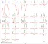 |
Fig. 2 Sr v lines in the observation (gray line) of RE 0503−289, labeled with their wavelengths from Table A.17. The thick, red spectrum is calculated from our best model with a Sr mass fraction of 6.5 × 10⁻⁴. The dashed, green line shows a synthetic spectrum calculated without Sr. In cases of Sr vλ 942.943 Å and Sr vλ 1412.959 Å, the red, dashed lines show two synthetic spectra calculated with Sr abundances that were increased and decreased by 0.3 dex. The vertical bar indicates 10% of the continuum flux. Identified lines are marked. “is” denotes interstellar. |
Sr iv:
we considered interaction among the configurations 4s24p5, 4s24p45p, 4s24p46p, 4s24p44f, 4s24p45f, 4s24p46f, 4s24p46h, 4s4p54d, 4s4p55d, 4s4p56d, 4s4p55s, 4s4p56s, 4s4p55g, 4s4p56g, 4s24p34d2, 4s24p34f2, and 4p64f for the odd parity, and 4s4p6, 4s24p44d, 4s24p45d, 4s24p46d, 4s24p45s, 4s24p46s, 4s24p47s, 4s24p45g, 4s24p46g, 4s4p54f, 4s4p55f, 4s4p56f, 4s4p55p, 4s4p56p, 4s4p56h, 4p64d, and 4p65s for the even parity. The core-polarization parameters were the dipole polarizability of a Ni-like Sr ix ionic core as reported by Johnson et al. (1983), that is, αd = 0.13 au, and the cut-off radius corresponding to the HFR mean value ⟨ r ⟩ of the outermost core orbital (3d), i.e., rc = 0.49 au. Using experimental energy levels compiled by Sansonetti (2012), the radial integrals (average energy, Slater, spin-orbit and effective interaction parameters) of 4p5, 4p45p, 4p46p, 4p44f, 4p45f, 4p46h, 4s4p54d, 4s4p6, 4p44d, 4p45d, 4p46d, 4p45s, 4p46s, 4p47s, 4p45g, and 4p46g configurations were optimized by a least-squares fitting procedure in which the mean deviations with experimental data were found to be equal to 145 cm-1 for the odd parity and 150 cm-1 for the even parity.
Sr v:
the HFR method was used with, as interacting configurations, 4s24p4, 4s24p35p, 4s24p36p, 4s24p34f, 4s24p35f, 4s24p36f, 4s24p36h, 4s4p44d, 4s4p45d, 4s4p46d, 4s4p45s, 4s4p46s, 4s4p45g, 4s4p46g, 4s24p24d2, 4s24p24f2, 4p6, and 4p54f for the even parity, and 4s4p5, 4s24p34d, 4s24p35d, 4s24p36d, 4s24p35s, 4s24p36s, 4s24p35g, 4s24p36g, 4s4p44f, 4s4p45f, 4s4p46f, 4s4p45p, 4s4p46p, 4s4p46h, 4p54d, and 4p55s for the odd parity. Core-polarization effects were estimated using the same αd and rc values as those considered in Sr iv. The radial integrals corresponding to 4p4, 4p35p, 4s4p5, 4p34d, 4p35d, 4p35s, and 4p36s were adjusted to reproduce at best the experimental energy levels tabulated by Sansonetti (2012). We note that the few levels reported by this author as belonging to the 4p34f and 4p35f configurations were not included in the fitting process because it was found that most of those levels were strongly mixed with states of experimentally unknown configurations, such as 4s4p44d, 4p36p, 4p24d2, and 4s4p45s. It was then extremely difficult to establish an unambiguous correspondence between the calculated and experimental energies. For the levels considered in our semi-empirical adjustment, we found mean deviations equal to 138 cm-1 and 231 cm-1 in even and odd parities, respectively.
Sr vi:
the configurations included in the HFR model were 4s24p3, 4s24p25p, 4s24p26p, 4s24p24f, 4s24p25f, 4s24p26f, 4s24p26h, 4s4p34d, 4s4p35d, 4s4p36d, 4s4p35s, 4s4p36s, 4s4p35g, 4s4p36g, 4s24p4d2, 4s24p4f2, 4p5, and 4p44f for the odd parity, and 4s4p4, 4s24p24d, 4s24p25d, 4s24p26d, 4s24p25s, 4s24p26s, 4s24p25g, 4s24p26g, 4s4p34f, 4s4p35f, 4s4p36f, 4s4p35p, 4s4p36p, 4s4p36h, 4p44d, and 4p45s for the even parity. The same core-polarization parameters as those used for Sr iv were considered while the fitting process was performed with the few experimental energy levels listed in the compilation of Sansonetti (2012) for optimizing the radial parameters of 4p3, 4s4p4, and 4p25s configurations, leading to mean deviations equal to 13 cm-1 (odd parity) and 32 cm-1 (even parity).
Sr vii:
a model similar to that of Sr vi was used, for which the 4s24p2, 4s24p5p, 4s24p6p, 4s24p4f, 4s24p5f, 4s24p6f, 4s24p6h, 4s4p24d, 4s4p25d, 4s4p26d, 4s4p25s, 4s4p26s, 4s4p25g, 4s4p26g, 4s24d2, 4s24f2, 4p4, and 4p34f even-parity configurations and the 4s4p3, 4s24p4d, 4s24p5d, 4s24p6d, 4s24p5s, 4s24p6s, 4s24p5g, 4s24p6g, 4s4p24f, 4s4p25f, 4s4p26f, 4s4p25p, 4s4p26p, 4s4p26h, 4p34d, and 4p35s odd-parity configurations were explicitly included in the HFR model. Here also, we used the same core-polarization parameters as those considered for Sr iv. The semi-empirical optimization process was carried out to adjust the radial parameters in 4p2, 4s4p3, and 4p5s with the experimental energy levels taken from Sansonetti (2012) giving rise to average deviations of 0 cm-1 and 247 cm-1 for even and odd parities, respectively.
Te vi:
the configuration interaction was considered among the following configurations: 4d105s, 4d106s, 4d107s, 4d105d, 4d106d, 4d107d, 4d95s2, 4d95p2, 4d95d2, 4d94f2, 4d95s5d, 4d95s6d, 4d95s6s, 4d94f5p, and 4d94f6p (even parity) and 4d105p, 4d106p, 4d107p, 4d104f, 4d105f, 4d106f, 4d107f, 4d95s5p, 4d95s6p, 4d95s5f, 4d95s6f, 4d94f5s, 4d94f6s, 4d94f5d, 4d94f6d (odd parity). The core-polarization parameters were those corresponding to a Rh-like Te viii ionic core, that is, αd = 1.15 au (Fraga et al. 1976) and rc ≡ ⟨ r ⟩ 4d = 0.95 au. The radial parameters of 4d105s, 4d106s, 4d105d, 4d95p2, 4d105p, 4d106p, and 4d95s5p configurations were optimized to minimize the differences between the computed Hamiltonian eigenvalues and the experimental energy levels published by Crooker & Joshi (1964), Dunne & O’Sullivan (1992), and Ryabtsev et al. (2007) giving rise to mean deviations of 89 m-1 (even parity) and 13 cm-1 (odd parity).
I vi:
thirty-two configurations were included in the HFR model used to compute the atomic structure, i.e., 5s2, 5p2, 5d2, 4f2, 5f2, 5s5d, 5s6d, 5s7d, 5s6s, 5s7s, 5p4f, 5p5f, 5p6f, 5d6s, 5d7s, 5d6d, and 5d7d for the even parity and 5s5p, 5s6p, 5s7p, 5s4f, 5s5f, 5s6f, 5s7f, 5p5d, 5p6d, 5p7d, 5p6s, 5p7s, 5d4f, 5d5f, and 5d6f for the odd parity. An ionic core of the type Pd-like I viii was considered to estimate the core-polarization effects with the parameters αd = 1.03 a.u. (Johnson et al. 1983) and rc≡⟨ r ⟩4d = 0.90 au. The semi-empirical optimization process was carried out to adjust the radial parameters in 5s2, 5p2, 5s5d, 5s6s, 5s7s, 5s5p, 5s6p, 5p5d, and 5p6s with the experimental energy levels taken from Tauheed et al. (1997) giving rise to average deviations of 72 cm-1 and 175 cm-1 for even and odd parities, respectively.
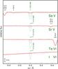 |
Fig. 3 STIS observation of G191−B2B (gray) compared with synthetic line profiles of Se vλ 1433.466 Å, Sr vλ 1413.882 Å, Te viλ 1313.874 Å, and I viλ 1219.395 Å. The models were calculated with four abundances of the respective elements, without (thin, blue), with 100 times (thick, red), 1000 times (short dashed, violet) and 10 000 times solar abundance (long dashed, green). |
The parameters adopted in our computations are summarized in Tables A.1–A.7 while calculated and available experimental energies are compared in Tables A.8–A.14, for Se v, Sr iv-vii,Te vi, and I vi, respectively. Tables A.15–A.21 give the newly computed weighted oscillator strengths (log gifik, i and k are the indexes of the lower and upper energy level, respectively) and transition probabilities (gkAki, in s-1) together with the numerical values (in cm-1) of the lower and upper energy levels and the corresponding wavelengths (in Å). In the final column of each table, we also give the cancellation factor, CF, as defined by Cowan (1981). We note that very low values of this factor (typically <0.05) indicate strong cancellation effects in the calculation of line strengths. In these cases, the corresponding log gifik and gkAki values could be very inaccurate and therefore need to be considered with some care. Figure B.1 shows the newly calculated log gifik values from the X-ray to the far infrared wavelength range.
Radiative decay rates for some transitions in the same ions as those considered in the present work were reported in previous papers. More precisely, for Se v, large-scale calculations for the 4s2–4s4p transitions were performed by Liu et al. (2006) using the multiconfiguration Dirac-Fock (MCDF) method and by Chen & Cheng (2010) using B-spline basis functions while the Relativistic Many Body Perturbation Theory (RMBPT), including the Breit interaction was used by Safronova & Safronova (2010) to compute oscillator strengths for transitions between even-parity 4s2, 4p2, 4s4d, 4d2, 4p4f, 4f2 and odd-parity 4s4p, 4s4f, 4p4d, 4d4f states. In Sr iv, transition probabilities and oscillator strengths for the electric dipole transitions involving the 4s24p5, 4s24p44d and 4s4p6 configurations were obtained using the multiconfiguration Dirac-Fock approach by Singh et al. (2013) and by Aggarwal & Keenan (2014). These works were subsequently extended by Aggarwal & Keenan (2015) to transitions involving the 4s24p5, 4s24p44ℓ, 4s4p6, 4s24p45ℓ, 4s24p34d2, 4s4p54ℓ, and 4s4p55ℓ configurations. For Sr vi, relativistic quantum defect orbital (RQDO) and MCDF calculations of oscillator strengths were carried out by Charro & Martín (1998, 2005) for the 4p3–4p25s transition array while the same methods were used by Charro & Martín (2002, 2005) for investigating the 4p2–4p5s transitions in Sr vii. In the case of Te vi, Chou & Johnson (1997) performed third-order relativistic many-body perturbation theory (MBPT) calculations to evaluate the rates for 5s–5p transitions while Migdalek & Garmulewicz (2000) used a relativistic ab initio model potential approach with explicit local exchange to produce oscillator strengths. In the same ion, the 5s–5p transition rates were also computed by Głowacki & Migdałek (2009) who employed a configuration-interaction method with numerical Dirac-Fock wave functions generated with noninteger outermost core shell occupation number while transition probabilities for 5s–5p, 5p–5d, 4f–5d, and 5d–5f transitions were calculated by Ivanova (2011). Finally, for I vi, the oscillator strengths of the allowed and spin-forbidden 5s21S0–5s5p 1,3P1 transitions were evaluated by Biémont et al. (2000) using the relativistic Hartree-Fock approach, including a core-polarization potential, and the MCDF method, as well as by Glowacki & Migdalek (2003) who used a relativistic configuration-interaction method with numerical Dirac-Fock wavefunctions generated with an ab initio model potential allowing for core-valence correlation.
In order to estimate the overall reliability of the new atomic data obtained in the present work, we have compared them with some of the most recent and the most extensive calculations available in literature, selected among those listed hereabove. More particularly, in Se v, we noticed that our oscillator strengths were in excellent agreement (within a few percent) with the RMBPT values published by Safronova & Safronova (2010). In the case of Sr iv, we found a general agreement of about 20−30% between our results and the oscillator strengths published by Aggarwal & Keenan (2015), this agreement reaching even 10% for the most intense lines. For Te vi, the mean ratio between our transition probabilities and the few values reported by Ivanova (2011) was found to be equal to 1.18 while, for I vi, a very good agreement (within 10%) was observed when comparing the gf-values obtained in the present work with those computed by Biémont et al. (2000) using either a relativistic Hartree-Fock or an MCDF model, taking core-valence correlation effects into account. All these comparisons allowed us to conclude that the accuracy of the new atomic data listed in the present paper should be about 20%, at least for the strongest lines.
Identified Se v, Sr v, Te vi, and I vi lines in the UV spectrum of RE 0503−289.
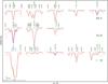 |
Fig. 4 As Fig. 2, for Se v (top, mass fraction of 1.6 ± 1.0 × 10⁻³ in the model), Te vi (middle, 2.5 × 10⁻⁴), and I vi (bottom, 1.4 × 10⁻⁵) lines. Abundance dependencies (±0.3 dex, red, dashed lines) are demonstrated for Se vλ 1454.292 Å, Te viλ 951.021 Å, and I viλ 1057.530 Å. |
4. Results
In the FUSE and HST/STIS observations of RE 0503−289, we newly identified 23 Sr v lines, listed in Table 2 which complements Table A.1 of Hoyer et al. (2017). Many more weak Sr v lines are visible in our model spectra that are not detectable in the noise of the available observations. The models show that the strongest Sr vi lines are located in the extreme ultraviolet (EUV) and X-ray wavelength range while Sr iv lines are too weak in general and fade within the noise of the available observations. The observed Sr v lines are well reproduced by our model calculated with a mass fraction of 6.5 × 10⁻⁴ (Fig. 2). To estimate the abundance uncertainty from the error propagation of Teff and log g, we evaluated models at the error limits (Teff = 70 000 ± 2000 K, log g = 7.5 ± 0.1) and found that it is smaller than 0.1 dex. To consider the abundance uncertainties of other metals and the impact of their background opacities, we finally adopted a Sr mass fraction of 6.5 × 10⁻⁴ with an uncertainty of 0.2 dex (Fig. 2 shows exemplarily the abundance dependence of two lines in a [−0.3 dex, +0.3 dex] abundance interval). The determined Sr abundance matches well the abundance pattern of trans-iron elements in RE 0503−289 (Fig. 1). Their extreme overabundances are the result of efficient radiative levitation (Rauch et al. 2016a).
Five Se v, three Te vi, and four I vi lines are used for the abundance determination of these elements (Fig. 4). We measured mass fractions of 1.6 × 10⁻³, 2.5 × 10⁻⁴, and 1.4 × 10⁻⁵ for Se, Te, and I, respectively. These agree well with the expectations from the abundance pattern of trans-iron elements in RE 0503−289 (Fig. 1).
A very weak impact of Se, Sr, Te, and I lines is noticeable in the EUV wavelength range. The so-called EUV problem, that is, the flux discrepancy between model and observation in this wavelength range (cf., Hoyer et al. 2017) is, however, not significantly reduced. We note that Preval et al. (2017) showed recently that improved, larger photoionization cross-section of Ni can reduce this discrepancy.
The search for Se, Sr, Te, and I lines in the FUSE and HST/STIS observations of G191−B2B was entirely negative. Figure 3 shows the most prominent lines that are predicted by our models, namely Se vλ 1433.466 Å (log gifik value of 0.16), Sr vλ 1413.882 Å (0.82), Te viλ 1313.874 Å (−0.05), and I viλ 1219.395 Å (−0.63). For all these elements, the upper abundance limit is ≈100 times the solar abundance.
Acknowledgments
T.R. and D.H. are supported by the German Aerospace Center (DLR, grants 05 OR 1507 and 50 OR 1501, respectively). The GAVO project had been supported by the Federal Ministry of Education and Research (BMBF) at Tübingen (05 AC 6 VTB, 05 AC 11 VTB) and is funded at Heidelberg (05 AC 11 VH3). Financial support from the Belgian FRS-FNRS is also acknowledged. P.Q. is research director of this organization. Some of the data presented in this paper were obtained from the Mikulski Archive for Space Telescopes (MAST). STScI is operated by the Association of Universities for Research in Astronomy, Inc., under NASA contract NAS5-26555. Support for MAST for non-HST data is provided by the NASA Office of Space Science via grant NNX09AF08G and by other grants and contracts. The TIRO (http://astro.uni-tuebingen.de/~TIRO), TMAD (http://astro.uni-tuebingen.de/~TMAD), and TOSS (http://astro.uni-tuebingen.de/~TOSS) services were constructed as part of the Tübingen project of the German Astrophysical Virtual Observatory (GAVO, http://www.g-vo.org). This research has made use of NASA’s Astrophysics Data System and the SIMBAD database, operated at CDS, Strasbourg, France.
References
- Aggarwal, K. M., & Keenan, F. P. 2014, Phys. Scr., 89, 125404 [NASA ADS] [CrossRef] [Google Scholar]
- Aggarwal, K. M., & Keenan, F. P. 2015, At. Data Nucl. Data Tables, 105, 9 [CrossRef] [Google Scholar]
- Asplund, M., Grevesse, N., Sauval, A. J., & Scott, P. 2009, ARA&A, 47, 481 [NASA ADS] [CrossRef] [Google Scholar]
- Biémont, E., Fischer, C. F., Godefroid, M. R., Palmeri, P., & Quinet, P. 2000, Phys. Rev. A, 62, 032512 [NASA ADS] [CrossRef] [Google Scholar]
- Charro, E., & Martín, I. 1998, A&AS, 131, 523 [NASA ADS] [CrossRef] [EDP Sciences] [Google Scholar]
- Charro, E., & Martín, I. 2002, A&A, 395, 719 [NASA ADS] [CrossRef] [EDP Sciences] [Google Scholar]
- Charro, E., & Martín, I. 2005, Int. J. Quantum Chem., 104, 446 [NASA ADS] [CrossRef] [Google Scholar]
- Chen, M. H., & Cheng, K. T. 2010, J. Phys. B, 43, 074019 [NASA ADS] [CrossRef] [Google Scholar]
- Chou, H.-S., & Johnson, W. R. 1997, Phys. Rev. A, 56, 2424 [NASA ADS] [CrossRef] [Google Scholar]
- Churilov, S. S., & Joshi, Y. N. 1995, Phys. Scr., 51, 196 [NASA ADS] [CrossRef] [Google Scholar]
- Cowan, R. D. 1981, The theory of atomic structure and spectra (Berkeley, CA: University of California Press) [Google Scholar]
- Crooker, A. M., & Joshi, Y. N. 1964, J. Opt. Soc. Am., 54, 553 [CrossRef] [Google Scholar]
- Dreizler, S., & Werner, K. 1996, A&A, 314, 217 [NASA ADS] [Google Scholar]
- Dunne, P., & O’Sullivan, G. 1992, J. Phys. B, 25, L593 [CrossRef] [Google Scholar]
- Fraga, S., Karwowski, J., & Saxena, K. M. S. 1976, Handbook of Atomic Data (Amsterdam: Elsevier) [Google Scholar]
- Glowacki, L., & Migdalek, J. 2003, J. Phys. B At. Mol. Phys., 36, 3629 [NASA ADS] [CrossRef] [Google Scholar]
- Głowacki, L., & Migdałek, J. 2009, Phys. Rev. A, 80, 042505 [NASA ADS] [CrossRef] [Google Scholar]
- Grevesse, N., Scott, P., Asplund, M., & Sauval, A. J. 2015, A&A, 573, A27 [NASA ADS] [CrossRef] [EDP Sciences] [Google Scholar]
- Hoyer, D., Rauch, T., Werner, K., Kruk, J. W., & Quinet, P. 2017, A&A, 598, A135 [NASA ADS] [CrossRef] [EDP Sciences] [Google Scholar]
- Ivanova, E. P. 2011, Atomic Data and Nuclear Data Tables, 97, 1 [NASA ADS] [CrossRef] [Google Scholar]
- Johnson, W. R., Kolb, D., & Huang, K.-N. 1983, Atomic Data and Nuclear Data Tables, 28, 333 [Google Scholar]
- Lemoine, M., Vidal-Madjar, A., Hébrard, G., et al. 2002, ApJS, 140, 67 [NASA ADS] [CrossRef] [Google Scholar]
- Liu, Y., Hutton, R., Zou, Y., Andersson, M., & Brage, T. 2006, J. Phys. B, 39, 3147 [NASA ADS] [CrossRef] [Google Scholar]
- McCook, G. P., & Sion, E. M. 1999a, ApJS, 121, 1 [NASA ADS] [CrossRef] [Google Scholar]
- McCook, G. P., & Sion, E. M. 1999b, VizieR Online Data Catalog, 3210, [Google Scholar]
- Migdalek, J., & Garmulewicz, M. 2000, J. Phys. B, 33, 1735 [NASA ADS] [CrossRef] [Google Scholar]
- Müller-Ringat, E. 2013, Dissertation, University of Tübingen, Germany, http://nbn-resolving.de/urn:nbn:de:bsz:21-opus-67747 [Google Scholar]
- Preval, S. P., Barstow, M. A., Badnell, N. R., Hubeny, I., & Holberg, J. B. 2017, MNRAS, 465, 269 [NASA ADS] [CrossRef] [Google Scholar]
- Quinet, P., Palmeri, P., Biémont, É., et al. 1999, MNRAS, 307, 934 [NASA ADS] [CrossRef] [EDP Sciences] [Google Scholar]
- Quinet, P., Palmeri, P., Biémont, É., et al. 2002, J. Alloys Comp., 344, 255 [CrossRef] [Google Scholar]
- Rao, K. R., & Badami, J. S. 1931, Proc. Roy. Soc. Lond. A: Math., Phys. Eng. Sci., 131, 154 [CrossRef] [Google Scholar]
- Rauch, T., & Deetjen, J. L. 2003, in Stellar Atmosphere Modeling, eds. I. Hubeny, D. Mihalas, & K. Werner, ASP Conf. Ser., 288, 103 [Google Scholar]
- Rauch, T., Werner, K., Biémont, É., Quinet, P., & Kruk, J. W. 2012, A&A, 546, A55 [NASA ADS] [CrossRef] [EDP Sciences] [Google Scholar]
- Rauch, T., Werner, K., Bohlin, R., & Kruk, J. W. 2013, A&A, 560, A106 [NASA ADS] [CrossRef] [EDP Sciences] [Google Scholar]
- Rauch, T., Werner, K., Quinet, P., & Kruk, J. W. 2014a, A&A, 564, A41 [NASA ADS] [CrossRef] [EDP Sciences] [Google Scholar]
- Rauch, T., Werner, K., Quinet, P., & Kruk, J. W. 2014b, A&A, 566, A10 [NASA ADS] [CrossRef] [EDP Sciences] [Google Scholar]
- Rauch, T., Werner, K., Quinet, P., & Kruk, J. W. 2015, A&A, 577, A6 [NASA ADS] [CrossRef] [EDP Sciences] [Google Scholar]
- Rauch, T., Quinet, P., Hoyer, D., et al. 2016a, A&A, 587, A39 [NASA ADS] [CrossRef] [EDP Sciences] [Google Scholar]
- Rauch, T., Quinet, P., Hoyer, D., et al. 2016b, A&A, 590, A128 [NASA ADS] [CrossRef] [EDP Sciences] [Google Scholar]
- Rauch, T., Gamrath, S., Quinet, P., et al. 2017, A&A, 599, A142 [NASA ADS] [CrossRef] [EDP Sciences] [Google Scholar]
- Ryabtsev, A. N., Churilov, S. S., & Kononov, É. Y. 2007, Opt. Spectrosc., 102, 354 [NASA ADS] [CrossRef] [Google Scholar]
- Safronova, U. I., & Safronova, M. S. 2010, J. Phys. B, 43, 074025 [NASA ADS] [CrossRef] [Google Scholar]
- Sansonetti, J. E. 2012, J. Phys. Chem. Ref. Data, 41, 013102 [NASA ADS] [CrossRef] [Google Scholar]
- Scott, P., Asplund, M., Grevesse, N., Bergemann, M., & Sauval, A. J. 2015a, A&A, 573, A26 [NASA ADS] [CrossRef] [EDP Sciences] [Google Scholar]
- Scott, P., Grevesse, N., Asplund, M., et al. 2015b, A&A, 573, A25 [NASA ADS] [CrossRef] [EDP Sciences] [Google Scholar]
- Singh, A. K., Aggarwal, S., & Mohan, M. 2013, Phys. Scr., 88, 035301 [NASA ADS] [CrossRef] [Google Scholar]
- Tauheed, A., Joshi, Y. N., & Pinnington, E. H. 1997, Phys. Scr., 56, 289 [NASA ADS] [CrossRef] [Google Scholar]
- Werner, K., Deetjen, J. L., Dreizler, S., et al. 2003, in Stellar Atmosphere Modeling, eds. I. Hubeny, D. Mihalas, & K. Werner, ASP Conf. Ser., 288, 31 [Google Scholar]
- Werner, K., Dreizler, S., & Rauch, T. 2012a, Astrophysics Source Code Library [record ascl:1212.015] [Google Scholar]
- Werner, K., Rauch, T., Ringat, E., & Kruk, J. W. 2012b, ApJ, 753, L7 [NASA ADS] [CrossRef] [Google Scholar]
Appendix A: Additional tables
Radial parameters (in cm-1) adopted for the calculations in Se v.
Radial parameters (in cm-1) adopted for the calculations in Sr iv.
Radial parameters (in cm-1) adopted for the calculations in Sr v.
Radial parameters (in cm-1) adopted for the calculations in Sr vi.
Radial parameters (in cm-1) adopted for the calculations in Sr vii.
Radial parameters (in cm-1) adopted for the calculations in Te vi.
Radial parameters (in cm-1) adopted for the calculations in I vi.
Comparison between available experimental and calculated energy levels in Se v.
Comparison between available experimental and calculated energy levels in Sr iv.
Comparison between available experimental and calculated energy levels in Sr v.
Comparison between available experimental and calculated energy levels in Sr vi.
Comparison between available experimental and calculated energy levels in Sr vii.
Comparison between available experimental and calculated energy levels in Te vi.
Comparison between available experimental and calculated energy levels in I vi.
Calculated HFR oscillator strengths (log gifik) and transition probabilities (gkAki) in Se v.
Calculated HFR oscillator strengths (log gifik) and transition probabilities (gkAki) in Sr iv.
Calculated HFR oscillator strengths (log gifik) and transition probabilities (gkAki) in Sr v.
Calculated HFR oscillator strengths (log gifik) and transition probabilities (gkAki) in Sr vi.
Calculated HFR oscillator strengths (log gifik) and transition probabilities (gkAki) in Sr vii.
Calculated HFR oscillator strengths (log gifik) and transition probabilities (gkAki) in Te vi. CF is the absolute value of the cancellation factor as defined by Cowan (1981).
Calculated HFR oscillator strengths (log gifik) and transition probabilities (gkAki) in I vi.
Appendix B: Additional figure
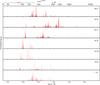 |
Fig. B.1 Newly calculated log gifik values of Se v, Sr iv–vii, Te vi, and I vi (from top to bottom). The log gifik values are normalized to the strongest line, matching 95% of the panels’ heights. The wavelength ranges of EUVE and of our FUSE and STIS spectra are indicated at the top. |
All Tables
Comparison between available experimental and calculated energy levels in Se v.
Comparison between available experimental and calculated energy levels in Sr iv.
Comparison between available experimental and calculated energy levels in Sr v.
Comparison between available experimental and calculated energy levels in Sr vi.
Comparison between available experimental and calculated energy levels in Sr vii.
Comparison between available experimental and calculated energy levels in Te vi.
Comparison between available experimental and calculated energy levels in I vi.
Calculated HFR oscillator strengths (log gifik) and transition probabilities (gkAki) in Se v.
Calculated HFR oscillator strengths (log gifik) and transition probabilities (gkAki) in Sr iv.
Calculated HFR oscillator strengths (log gifik) and transition probabilities (gkAki) in Sr v.
Calculated HFR oscillator strengths (log gifik) and transition probabilities (gkAki) in Sr vi.
Calculated HFR oscillator strengths (log gifik) and transition probabilities (gkAki) in Sr vii.
Calculated HFR oscillator strengths (log gifik) and transition probabilities (gkAki) in Te vi. CF is the absolute value of the cancellation factor as defined by Cowan (1981).
Calculated HFR oscillator strengths (log gifik) and transition probabilities (gkAki) in I vi.
All Figures
|
Fig. 1 Solar abundances (Asplund et al. 2009; Scott et al. 2015a,b; Grevesse et al. 2015, thick line; the dashed lines connect the elements with even and with odd atomic number) compared with the determined photospheric abundances of RE 0503−289 (red squares, Dreizler & Werner 1996; Rauch et al. 2012, 2014a,b, 2015, 2016a,b, 2017, and this work). The uncertainties of the WD abundances are about 0.2 dex in general. Arrows indicate upper limits. Top panel: abundances given as logarithmic mass fractions. Bottom panel: abundance ratios to respective solar values, [X] denotes log (fraction/solar fraction) of species X. The dashed, green line indicates solar abundances. |
| In the text | |
|
Fig. 2 Sr v lines in the observation (gray line) of RE 0503−289, labeled with their wavelengths from Table A.17. The thick, red spectrum is calculated from our best model with a Sr mass fraction of 6.5 × 10⁻⁴. The dashed, green line shows a synthetic spectrum calculated without Sr. In cases of Sr vλ 942.943 Å and Sr vλ 1412.959 Å, the red, dashed lines show two synthetic spectra calculated with Sr abundances that were increased and decreased by 0.3 dex. The vertical bar indicates 10% of the continuum flux. Identified lines are marked. “is” denotes interstellar. |
| In the text | |
|
Fig. 3 STIS observation of G191−B2B (gray) compared with synthetic line profiles of Se vλ 1433.466 Å, Sr vλ 1413.882 Å, Te viλ 1313.874 Å, and I viλ 1219.395 Å. The models were calculated with four abundances of the respective elements, without (thin, blue), with 100 times (thick, red), 1000 times (short dashed, violet) and 10 000 times solar abundance (long dashed, green). |
| In the text | |
|
Fig. 4 As Fig. 2, for Se v (top, mass fraction of 1.6 ± 1.0 × 10⁻³ in the model), Te vi (middle, 2.5 × 10⁻⁴), and I vi (bottom, 1.4 × 10⁻⁵) lines. Abundance dependencies (±0.3 dex, red, dashed lines) are demonstrated for Se vλ 1454.292 Å, Te viλ 951.021 Å, and I viλ 1057.530 Å. |
| In the text | |
|
Fig. B.1 Newly calculated log gifik values of Se v, Sr iv–vii, Te vi, and I vi (from top to bottom). The log gifik values are normalized to the strongest line, matching 95% of the panels’ heights. The wavelength ranges of EUVE and of our FUSE and STIS spectra are indicated at the top. |
| In the text | |
Current usage metrics show cumulative count of Article Views (full-text article views including HTML views, PDF and ePub downloads, according to the available data) and Abstracts Views on Vision4Press platform.
Data correspond to usage on the plateform after 2015. The current usage metrics is available 48-96 hours after online publication and is updated daily on week days.
Initial download of the metrics may take a while.