| Issue |
A&A
Volume 603, July 2017
|
|
|---|---|---|
| Article Number | A101 | |
| Number of page(s) | 12 | |
| Section | The Sun | |
| DOI | https://doi.org/10.1051/0004-6361/201730413 | |
| Published online | 19 July 2017 | |
Measuring the magnetic field of a trans-equatorial loop system using coronal seismology⋆
1 UCL-Mullard Space Science Laboratory, Holmbury House, Holmbury St. Mary, Dorking, Surrey, RH5 6NT UK
e-mail: david.long@ucl.ac.uk
2 Mathematics, Physics and Electrical Engineering, Northumbria University, Newcastle Upon Tyne, NE1 8ST, UK
3 Instituto de Astronomía y Física del Espacio (IAFE), CONICET-UBA, Buenos Aires, Argentina
4 Facultad de Ciencias Exactas y Naturales (FCEN), UBA, Buenos Aires, Argentina
Received: 10 January 2017
Accepted: 28 March 2017
Context. EIT waves are freely-propagating global pulses in the low corona which are strongly associated with the initial evolution of coronal mass ejections (CMEs). They are thought to be large-amplitude, fast-mode magnetohydrodynamic waves initially driven by the rapid expansion of a CME in the low corona.
Aims. An EIT wave was observed on 6 July 2012 to impact an adjacent trans-equatorial loop system which then exhibited a decaying oscillation as it returned to rest. Observations of the loop oscillations were used to estimate the magnetic field strength of the loop system by studying the decaying oscillation of the loop, measuring the propagation of ubiquitous transverse waves in the loop and extrapolating the magnetic field from observed magnetograms.
Methods. Observations from the Atmospheric Imaging Assembly onboard the Solar Dynamics Observatory (SDO/AIA) and the Coronal Multi-channel Polarimeter (CoMP) were used to study the event. An Empirical Mode Decomposition analysis was used to characterise the oscillation of the loop system in CoMP Doppler velocity and line width and in AIA intensity.
Results. The loop system was shown to oscillate in the 2nd harmonic mode rather than at the fundamental frequency, with the seismological analysis returning an estimated magnetic field strength of ≈ 5.5 ± 1.5 G. This compares to the magnetic field strength estimates of ≈1–9 G and ≈3–9 G found using the measurements of transverse wave propagation and magnetic field extrapolation respectively.
Key words: Sun: corona / Sun: magnetic fields / Sun: oscillations
A movie associated to Figs. 1 and 2 is available at http://www.aanda.org
© ESO, 2017
1. Introduction
First observed by the Solar and Heliospheric Observatory (SOHO; Domingo et al. 1995), many theories have been proposed to interpret globally-propagating coronal disturbances (commonly called EIT waves). Taking their name from the Extreme ultraviolet Imaging Telescope (EIT; Delaboudinière et al. 1995) onboard SOHO, they are typically observed as radially expanding bright features associated with the onset of a coronal mass ejection (CME) that can traverse the solar disk in under an hour (e.g., Moses et al. 1997; Dere et al. 1997; Thompson et al. 1998). After almost 20 yr of detailed investigation and debate, a consensus is finally being reached with regard to the physics underpinning their evolution, thanks to the improved temporal and spatial resolution of the Solar and Terrestrial Relations Observatory (STEREO; Kaiser et al. 2008) and more recently the Solar Dynamics Observatory (SDO; Pesnell et al. 2012).
The multitude of theories proposed to explain this phenomenon is mainly the result of conflicting observations (cf. Long et al. 2017). Initially interpreted as the coronal counterpart of the chromospheric Moreton-Ramsey wave (Moreton 1960; Moreton & Ramsey 1960), EIT waves were treated as fast-mode magneto-acoustic (MHD) waves following the example of Uchida (1968). However, issues with this interpretation were raised by observations of stationary brightenings at the edges of coronal holes (cf. Delannée & Aulanier 1999). These observations led to the suggestion that EIT waves were not true waves but instead were a brightening produced by the restructuring of the magnetic field during the eruption of a CME. It was proposed that this brightening was alternatively produced by Joule heating at the interface between the magnetic field of the erupting CME and the surrounding coronal magnetic field (Delannée 2000; Delannée et al. 2008), continuous reconnection of small-scale magnetic loops driven by the erupting CME (Attrill et al. 2007) or the stretching of magnetic field lines overlying an erupting flux rope (Chen et al. 2002, 2005). This last scenario was also supported by the relatively low observed speed of the disturbances (with an average speed of 200–400 km s-1 measured by Thompson & Myers 2009, using observations from SOHO/EIT).
However, these hypotheses have been undermined both by observations of reflection and refraction at coronal hole and active region boundaries (e.g., Thompson et al. 2000; Long et al. 2008; Veronig et al. 2008; Gopalswamy et al. 2009; Shen et al. 2013; Kienreich et al. 2013) as well as the higher speeds measured using STEREO (100–630 km s-1; Muhr et al. 2014) and SDO (vmean ≈ 644 km s-1; Nitta et al. 2013). Although initially analysed using the linearised fast-mode wave equations, observations of pulse dispersion and deceleration (Warmuth et al. 2004a,b; Long et al. 2011a,b) have led to their interpretation as large-amplitude simple waves (e.g., Vršnak & Lulić 2000a,b; Warmuth 2007; Vršnak & Cliver 2008) initially driven by the rapid expansion of the erupting CME in the low corona (Patsourakos et al. 2010) before propagating freely. Note that a number of different reviews by Gallagher & Long (2011), Zhukov (2011), Patsourakos & Vourlidas (2012), Liu & Ofman (2014) and more recently Warmuth (2015) discuss the different interpretations and the observations both supporting and contradicting them in detail.
More recently, the higher temporal and spatial resolution provided by the Atmospheric Imaging Assembly (AIA; Lemen et al. 2012) has revolutionised our understanding of EIT waves. These improved observations are providing clear evidence that the freely propagating EIT waves behave as waves, in principle allowing their observed characteristics to be used as diagnostics of the physical properties of the coronal regions through which they propagate (an approach called coronal seismology, e.g., Roberts et al. 1984; Ballai 2007) and estimate properties such as magnetic field strength (cf. Warmuth & Mann 2005; West et al. 2011; Kwon et al. 2013; Long et al. 2013). A similar approach may also be applied on a more local scale, using the forced oscillations of coronal loops initially driven by the impact of an EIT wave to determine properties such as their magnetic field strength or the energy of the wave-pulse (e.g., Ballai 2007; Ballai et al. 2008, 2011; Yang et al. 2013).
While the global nature of EIT waves greatly increases the chances of them interacting with coronal loops, these observations are dependent on a sufficiently high temporal and spatial resolution to be able to identify the oscillating loop. Despite its global field-of-view, SOHO/EIT did not have a sufficiently high temporal or spatial resolution to identify oscillating loops. This changed with the launch of the Transition Region And Coronal Explorer (TRACE; Handy et al. 1999), whose observations were used to show that the oscillation of a coronal loop may be used to estimate its magnetic field strength (e.g., Aschwanden et al. 1999; Nakariakov & Ofman 2001; Aschwanden & Schrijver 2011; Guo et al. 2015). Subsequent work extended the method to observations of oscillation in Doppler motion made by the Extreme ultraviolet Imaging Spectrometer (EIS; Culhane et al. 2007) onboard the Hinode spacecraft (e.g., Van Doorsselaere et al. 2008a).
In this paper, we estimate the magnetic field of a trans-equatorial loop system using multiple independent techniques. The first approach uses the oscillation of the loop system resulting from the impact of the global EUV wave-pulse, the second uses direct observations of the magnetic field made by the by the ground–based Coronal Multi–channel Polarimeter (CoMP) instrument (Tomczyk et al. 2008), while the third estimates the field strength using two independent magnetic field extrapolations from the photosphere. This paper builds on work previously presented at the International Astronomical Union (IAU) Symposium on Solar and Stellar Flares and Their Effects on Planets (described by Long et al. 2016), and represent a significant advance on the previously published proceedings paper. The observations are presented in Sect. 2, with the properties of the pulse and its interaction with the surrounding corona examined in Sects. 3 and 4 respectively. This interaction is then used to derive the magnetic field strength associated with a nearby transequatorial loop system in Sect. 5. Finally, some conclusions about the implication of these observations are drawn in Sect. 6.
2. Observations and data analysis
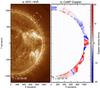 |
Fig. 1 Intensity image from SDO 193 Å (panel a)) and Doppler velocity from CoMP (panel b)). The dashed lines above the limb (at a height 1.09 R⊙) in both panels are used to make Fig. 3. The arc sector in the top right of panel a) shows the region used to get the density of the quiet Sun in Sect. 5.1. Note that the intensity image in panel a) has been enhanced using the Multi-scale Gaussian Normalisation technique of Morgan & Druckmüller (2014). The evolution of the 193 Å channel is shown in the left panel of the movie available online. |
The solar eruption studied here originated from NOAA active region AR 11514 on 6 July 2012 and was associated with a CME and a GOES X1.1 class flare which began at 23:01 UT. The event was well observed by multiple instruments including SDO/AIA and CoMP (see Fig. 1), providing an opportunity to study the eruption in detail. As with the event of 25 February 2014 previously studied by Long et al. (2015), the global EUV wave observed here did not propagate isotropically (see Fig. 2). Instead, due to the presence of the adjacent active regions AR 11515 to the East and ARs 11513, 11516 and 11517 to the North, the EIT wave propagated mainly towards the south polar coronal hole along the limb as seen by SDO/AIA (this is shown in the movie attached to Fig. 1).
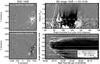 |
Fig. 2 Running difference images from the 193 Å passband of the eruption (panel a)) and the evolution of the wave (panel c)). The temporal evolution of the wave is shown in the right panel of the movie available online (showing the west half of the solar disk only). Panel b) shows a base-difference deprojected annulus image showing the eruption at 23:15:06 UT, with the vertical axis giving the height from Sun-centre and the horizontal axis giving the position angle clockwise from solar north (indicated by the dashed white line in panel a)). Panel d) shows a base-difference image of the temporal variation at a height of 1.09 R⊙ (indicated by the white dashed line in panel b)). The dashed white line in panel d) shows the fit to the leading edge of the propagating pulse. |
Designed to study the coronal magnetic field, CoMP provides Stokes-I measurements in the Fe xiii 10 747 Å and 10 798 Å emission lines with a field of view of 2.8 R⊙ and an image size of 620 × 620 pixels. This gives an image sample size of ~4.25 arcsec pixel-1 at ~30 s cadence (cf. Tian et al. 2013). Although the seeing was not good enough for this event to estimate the full Stokes parameters (S. Tomczyk, priv. comm.), the Stokes-I measurements can be fitted using a least-squares Gaussian fit to estimate the line intensity, width and central wavelength for each pixel. This allows the plasma parameters to be studied, giving an estimate of the temporal variations in Doppler motion and line width in the low corona.
3. Pulse properties
As the EIT wave was observed to propagate along the solar limb from the erupting active region towards the south pole, it was not possible to use the Coronal Pulse Identification and Tracking Algorithm (CorPITA; Long et al. 2014) to study the propagation of the pulse. Instead, following Long et al. (2015), a polar deprojection was used to determine the variation in pulse kinematics across a height range from 1.01–1.12 R⊙ (as shown in Fig. 2). This height range was chosen because above ≈1.12 R⊙ the pulse becomes very faint in the SDO/AIA images while the CoMP observations become noisy and prone to missing data, making direct comparisons between the instruments difficult.
The leading edge of the wave-pulse was manually identified and fitted using a quadratic model at each height across the entire range, as shown for height 1.09 R⊙ in Fig. 2, with the process repeated 10 times in each case to minimise uncertainty. The pulse was found to have a velocity ranging from 607–1583 km s-1, with a mean velocity of ≈1106 ± 314 km s-1 and an acceleration ranging from − 376–− 19 m s-2, with a mean acceleration of ≈− 207 ± 107 m s-2. These estimates are much higher than the average EIT wave speed measured by Nitta et al. (2013), indicating that the pulse measured here was quite fast. The pulse also exhibited clear deceleration, evidence of broadening and was associated with a Type II radio burst (cf. Long et al. 2017), suggesting that it was a large amplitude wave pulse.
For such a fast and intense pulse it is possible to follow the approach of Long et al. (2015) and estimate its initial energy using the Sedov-Taylor approximation (Taylor 1950a,b; Sedov 1959). Although this assumes a spherically symmetric blast wave emanating from a point source (which is not strictly valid here), Grechnev et al. (2008, 2011) and Long et al. (2015) found that the approach is suitable for analysing the onset stage of pulses being initially driven over a very short time period before propagating freely, as with the event studied here. Long et al. (2015) have also shown that the Sedov-Taylor relation provides an excellent estimate of the initial energy of the eruption assuming a blast wave propagating through a medium of variable density. Using this approach, the initial energy of the pulse was estimated to be ~8.6 × 1031 erg, comparable to the previous estimate made by Long et al. (2015). While this is consistent with the observations of high initial velocity and strong pulse deceleration, it is most likely an overestimate of the true energy of the wave-pulse. As noted by Long et al. (2015), the Sedov-Taylor relation assumes a spherical blast wave emanating from a source point, which is not the case here and does not include the effect of the coronal magnetic field. As a result, this estimate should be considered as a first order approximation of the energy of the pulse.
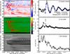 |
Fig. 3 Temporal variation in CoMP Doppler velocity (panel a)) and line width (panel c)) and AIA 193 Å percentage base difference (PBD) intensity (panel e)) at a height of 1.09 R⊙ (shown by the dashed line in panels a) and b) of Fig. 1). Panels b), d) and f) show the temporal variation in Doppler velocity, line width and AIA PBD intensity along the dashed line indicated in panels a), c) and e). The oscillatory behaviour of the loop system is very clear in the Doppler motion (panels a) and b)), indicating motion to-and-from the observer, while the impact of the pulse and subsequent evacuation of plasma into the CME is apparent in the line width (panels c) and d)) and plane-of-sky AIA observations respectively (panels e) and f)), as described in the text. The solid blue line in panel b) indicates a fit to the data using the damped cosine model described in Eq. (1). |
Although the pulse can be clearly identified in the AIA 193 Å intensity observations (e.g., Fig. 2), it was not as apparent in the CoMP intensity observations. This is clear from panel a of Fig. 3, where the effects of the pulse can be seen in Doppler velocity, but not the pulse itself. As a result, the CoMP observations were used to study the effects of the pulse on the surrounding corona, with the AIA 193 Å observations used to estimate the pulse kinematics.
4. Interaction with trans-equatorial loop system
Although the Sedov-Taylor approximation assumes an isotropic expansion of the wave-pulse being studied, this is not the case here due to the trans-equatorial loop system to the north of the erupting active region. This is shown in Fig. 2 and the associated movie. While this feature restricts the propagation of the wave-pulse, the effects of the impact force a significant displacement of the trans-equatorial loop system from rest. This results in a large amplitude decaying oscillation in CoMP Doppler observations as the loop returns to its pre-impact position, as shown in detail in Fig. 3 at a specific location of the observed loop structure. As a result, it is possible to estimate the magnetic field of the loop system using a coronal seismology approach (e.g., Roberts et al. 1984; Van Doorsselaere et al. 2008a; Long et al. 2013).
The temporal variation in CoMP Doppler velocity and line width and AIA percentage base difference (PBD) intensity at a height of 1.09 R⊙ and for all polar angles are shown in the left panels a, c and e of Fig. 3. The pulse is clearest in the Doppler velocity and AIA PBD measurements (panels a and e), although there is a slight suggestion of variation in the line width measurements (panel c). The wave-pulse is first seen in the Doppler velocity observations at ≈23:04 UT, with a slightly blue-shifted edge moving northwards away from the erupting active region (located at ~110° clockwise from solar north). It can also be seen to move towards the south pole at roughly the same time, again observed as an initially slightly blue-shifted edge. A co-temporal faint bright feature can also be identified in the PBD measurements in panel e moving both north and south away from the source active region. Although there is some indication of a slight change in the line width shown in panel c at this time, there is no clear signature of a propagating front.
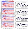 |
Fig. 4 Temporal variation in Doppler velocity at heights of 1.11, 1.12, 1.13 and 1.14 R⊙ for all polar angles (left column) along with its temporal profile measured at angles of 94°, 86°, 85° and 88° clockwise from solar north (right column). The solid blue lines in the right column indicate a fit to the data using the damped cosine model described in Eq. (1). |
Following the initial front, there is clear evidence of material being ejected with the erupting CME. This is apparent from the red-shifted outflow from the erupting active region apparent in the sector from 100–120° starting at ~23:07 UT and continuing for the rest of the time period shown. This corresponds to a drop in the PBD intensity (panel e of Fig. 3), indicating a drop in density and/or temperature as material is evacuated by the CME. This drop in intensity is also clear in panel f, which shows the temporal variation in PBD intensity at ~95° clockwise from solar north (as for panels b and d, shown by the dashed line in panel e).
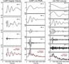 |
Fig. 5 Intrinsic Mode Functions derived from the time evolution of the Doppler velocity (left panels), line width (centre panels) and AIA PBD intensity (right panels), corresponding to the data in the right panels of Fig. 3. In each case the bottom panel shows the original signal (cf. Fig. 3b, d and f) with the upper panels giving the derived components. |
While the propagation of the pulse to the south of the erupting active region is relatively uninhibited, the propagation to the north is modified by a trans-equatorial loop system located between ~85–100° clockwise from solar north (as shown in Fig. 1). The variation in Doppler velocity with time in panel a of Fig. 3 shows that this loop system is relatively stable until the impact of the blue-shifted wave-pulse at ~23:05 UT. A more strongly blue-shifted feature is then observed between ~23:07 UT and ~23:17 UT along the profile in panel b, which is also characterised by a very strong co-temporal increase in line width (seen in panel d). This suggests turbulent behaviour (cf. Harra et al. 2009), and is consistent with the initial impact of the wave-pulse on the loop system followed by the outward motion of the associated erupting filament.
The effects of the impact of the wave-pulse on the trans-equatorial loop system may then be seen in panel a from ~23:17 UT onwards as it exhibits a series of alternating red- and blue-shifted features. This can be attributed to the loop system being displaced from its rest position by the impact of the wave-pulse and subsequently returning to rest via a decaying oscillation. This behaviour is shown most clearly in panel b of Fig. 3, which corresponds to the temporal Doppler velocity profile at an angle of 95° clockwise from solar north (indicated by the dashed line in panel a). It should also be noted that as the Doppler velocity in panel b begins to exhibit this strong oscillation, the line width drops dramatically to near the pre-event level, suggesting a near-uniform oscillation of the loop system.
This oscillatory behaviour in the Doppler velocity is consistent along the loop as shown in Fig. 4, which shows the variation in Doppler velocity at a set of sampled locations (height and polar angle) along the rest of the loop system. It is clear from the temporal evolution of the Doppler velocities shown in the left panels of Fig. 4 that the signal weakens above ~1.14 R⊙, with clear data drop-outs apparent at ~95–110°. While the amplitude of the oscillation can be seen to drop with increasing height, the period and damping time are comparable in all cases, suggesting that the values quoted in Fig. 3 are representative of the oscillation along the loop. These observations suggest that the wave-pulse impacts the leg of the loop system in the low corona (thus leading to the larger amplitude of the oscillation at lower heights). The consistent damping time also suggests that while the loop system is perturbed by the pulse impact, it stays relatively stable and is not opened by this impact. The mass of the loop system and hence the oscillation and associated damping coefficient therefore remain constant throughout the oscillation.
4.1. Empirical Mode Decomposition analysis
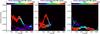 |
Fig. 6 Hilbert Huang Transform (HHT) spectra for the Doppler velocity (left column), line width (centre column) and PBD intensity (right column) corresponding to the IMFs shown in Fig. 5. Note that only the HHT of the IMF = 3 and residual, IMF = 3 and 4, and IMF = 4 and 5 are shown in the three cases, respectively. |
While the oscillatory behaviour of the Doppler velocity is very clear in panel b of Fig. 3, there is some indication of a comparable (albeit extremely faint) oscillation in the line width and PBD intensity shown in panels d and f. To determine if an oscillation was present, the temporal evolution of the different signals was examined using an Empirical Mode Decomposition (EMD; Huang et al. 1998; Quek et al. 2003) analysis. This technique decomposes the original signal into a series of Intrinsic Mode Functions (IMFs) and a residual, with the associated energy distribution represented by a Hilbert-Huang spectrum. The approach involves constructing a low- and a high-envelope from the series of maxima and minima of the signal, and then averaging the two envelopes. Under certain constraints, the resulting function is called an IMF and captures the fastest oscillating part in the signal. A new signal is then obtained by subtracting the IMF from the signal itself. This process is repeated until the updated signal shows no more oscillation, leaving the residual, (see, e.g. Stangalini et al. 2014, for more details). Since IMFs are time-dependent, a convenient way of representing their contribution to the signal at each time is to use an Hilbert transform as defined by Huang et al. (1998), which can be used to describe the time-evolution of the (instantaneous) frequency of each IMF.
The EMD analysis was applied to the Doppler velocity, line width and PBD intensity signals shown in panels b, d and f, respectively, of Fig. 3. Note that in the following analysis we focus on the impact of the wave-pulse on the trans-equatorial loop system and its resulting oscillation, leaving a more detailed study of the correlation of the various IMFs between the different signals for a dedicated future work.
Figure 5 shows the output from the EMD analysis, with the bottom panel for each column giving the original signal (black) and residual (red) while the upper panels give the corresponding IMFs. The left panels show that the Doppler velocity can be decomposed into three IMFs, with the oscillatory behavior mostly captured by IMF = 3, which reveals an almost constant frequency of 1.0 mHz up to about t = 3000 s. While this approach can provide a more accurate estimate of the frequency of the oscillation, the composing IMFs are not orthogonal functions, leading to the crosstalk observed in the second half of the time series for IMF = 2 and 3. The IMF = 2 contribution also shows the presence of a more complex component which is not purely oscillatory in nature. The residual also shows an oscillatory behavior on a longer period than the loop oscillation. However, the oscillation in the residual is not complete and therefore the residual is not considered to be an IMF. The difference between the oscillatory Doppler signal and this longer component is best seen using a Hilbert-Huang Transform (HHT) as shown in Fig. 6. The left panel here shows the HHT spectrum restricted to the residual and the IMF = 3. The spectral contribution of the oscillatory component from IMF = 3 is represented by the intense red strip around 1 mHz which stays almost constant in frequency until t ≃ 3000 s, before strongly damping and decreasing to 0.5 mHz, (cf. the left panel of Fig. 5). The residual contribution appears in this plot as a periodic, low-intensity component in the lower part of the spectrum at a frequency of 0.2 mHz.
The central panels of Fig. 5 show the decomposed IMF for the line width shown in panel d of Fig. 3. Here the high-frequency IMFs = 1 and 2 capture a transient nonlinear pulse in the time period ~600 <t< 1400 s which has a period much shorter than the loop oscillation and cannot be clearly identified in the Doppler signal (except for a small-amplitude trace in the IMF = 1 of the left-hand column of Fig. 5). The frequency of the IMF = 2 in Fig. 5 can be seen to chirp in time from ~1.5 to 3.5 mHz, whereas the evolution of the IMF = 1 is less clear. However for clarity neither IMF is included in Fig. 6. These signals are clearly different to the loop system damped oscillation (mostly captured in Fig. 5 by IMF = 3), which again reproduces the component of the oscillating loop system in the IMF = 3 of the Doppler velocity signal (although at a slightly more variable frequency between ~0.5 and 1 mHz, see the central panel in Fig. 6), and a lower frequency component at about 0.4 mHz.
The IMF decomposition of the AIA signal in the right panels of Fig. 5 shows the highest level of complexity, partly due to the higher cadence of the AIA signal which captures more time-scales than CoMP. Despite this, both loop-system oscillation components can be identified with a clear damping signature (e.g., IMF = 4), and the nonlinear signal due to the wave-pulse itself (e.g., IMF = 2). In the HHT shown in the far right panel of Fig. 6, the frequency of the oscillating mode is similar to the one generated by the IMF = 3 of the CoMP line-width signal, albeit relatively weaker. Similarly, the 0.2 mHz signal is also found in the PBD intensity from AIA. The effects of the higher AIA cadence are seen in the highest-frequency IMF = 1, which has the typical signature of noise and/or under-sampling (i.e., fluctuations on the highest frequency, whereas all higher IMFs are resolved signals).
The initial transients apparent in the IMF = 1 of the CoMP line width and in the IMF = 2 of the AIA PBD intensity are very similar in both structure and timing. The transients occur at the time the pulse reaches the trans-equatorial loop system, and appear as an oscillating wave modulated by an envelope rather than as a damped oscillation. It is intriguing that exactly such a pattern was previously assumed as the internal structure of an EIT wave pulse by Long et al. (2011a) and we are therefore tempted to identify this transient signal as the pulse itself.
However, if our pulse velocity estimate measured in Sect. 3 can also be applied at the front impacting the trans-equatorial loop system, this signal would indicate a pulse much broader than that observed. Therefore, we cannot unequivocally exclude that the observed transient signals are due to other nonlinear interactions between the pulse and loop systems. The case studied here is not optimal for discriminating between these possibilities and we leave such an analysis to a future work.
5. Magnetic field strength estimates
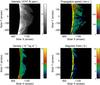 |
Fig. 7 The results of the magneto-seismology of propagating transverse waves. The top left panel shows the coronal loop as observed in 10 747 Å line centroid wavelength at 18:43 UT, with the measured propagation speeds of the transverse waves shown in the top right panel. The white contour over the intensity image shows the region in 10 798 Å that has adequate signal level. The lower left panel displays the estimates of plasma density from the 10 798 Å/10 747 Å ratio and the right hand panel shows the magnetic field estimate. |
The EMD analysis suggests that the oscillation of the loop system is consistent with the fast magneto-acoustic kink mode as modelled by Aschwanden et al. (1999), with the clear Doppler velocity signal indicating a large-scale motion of the loop system towards and away from the observer. Figure 5 shows a damped oscillatory component present in both the line width and PBD intensity signals that has a period comparable to that observed in the Doppler velocity signal. However, it is very small and is most likely due to the apparent brightening and dimming as the loop system moves towards and away from the observer (cf. Van Doorsselaere et al. 2008b). This interpretation also means that it may be possible to use the oscillation of the loop system to estimate its magnetic field via coronal seismology (Sect. 5.1).
Although CoMP was originally designed to measure the coronal magnetic field, the seeing was not good enough for this event to make measurements of the full Stokes-I, Q, U and V parameters. Instead, a magnetoseismology technique developed by Tomczyk et al. (2007) and Morton et al. (2015, 2016) was used to estimate the magnetic field strength of the loop system (Sect. 5.2). This approach does not require any oscillation of the loop system, allowing an independent verification of the values derived from the coronal seismology technique. To provide an additional independent verification, the magnetic field was also estimated using a pair of magnetic field extrapolations derived from both GONG and HMI magnetograms (Sect. 5.3).
5.1. Coronal seismology
The coronal seismology approach most commonly used to estimate the magnetic field within an oscillating coronal loop uses the damping of the loop as it returns to its original rest position to derive the period of oscillation. This is done by fitting the damped oscillation using an exponentially decreasing cosine function of the form, 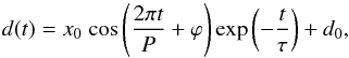 (1)where x0 is the amplitude, P is the period, ϕ is the phase, τ is the damping time and d0 is the equilibrium position. This model was applied to the variation in Doppler velocity shown in panel b of Fig. 3, with the resulting fit shown by the blue line and the fitted values given in the bottom right of the panel. It is clear that the model fits the observations very well, indicating that the assumption of a kink mode oscillation is consistent with the observations. The model was then applied to the Doppler velocity along the loop system, with Fig. 4 showing a representative sample of profiles with the blue line in each case showing the model fit to the data. It is clear that the oscillation is exhibited along the loop system at a range of heights and locations, with the model providing an excellent fit to the data in each case.
Although the oscillation of the loop system may be interpreted as as a kink mode wave as discussed in Sect. 4.1, it is not oscillating at the fundamental frequency. Instead, the out of phase Doppler signal observed between the legs of the loop system (apparent between ≈90−100° in the Doppler velocity plots shown in Figs. 3 and 4) and the lack of a signal at the top of the loop system suggest that it is oscillating at the 2nd harmonic frequency. The oscillation period can therefore be used to estimate the strength of the magnetic field of the loop using the equation, 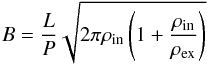 (2)where B is the magnetic field strength, L is the loop length, P is the period of the oscillation, ρin is the internal density of the loop system and ρex is the external density of the surrounding corona (cf. Roberts et al. 1984; Nakariakov & Ofman 2001; Aschwanden & Schrijver 2011).
The length of the loop was estimated by fitting an ellipse to the loop identified by visual inspection in the SDO/AIA observations. This was done using the 193 Å passband, with the images processed using the Multiscale Gaussian Normalisation technique of Morgan & Druckmüller (2014) to highlight the loop and make it easier to identify. The process was repeated ten times to reduce uncertainty, with the loop length estimated at 711 ± 8 Mm.
The density of the loop system and the surrounding corona were estimated using the regularised inversion technique of Hannah & Kontar (2013) assuming a temperature of ~1.5 MK (corresponding to the peak emission temperature of the 193 Å passband used to identify the wave-pulse). The spatial extent of the loop system was estimated using observations from the STEREO-A spacecraft to be ≈373 Mm. This was used as the line-of-sight along which to integrate the emission measure for both the internal and external densities of the loop system. The internal density of the loop system at the location used to identify the oscillation in Doppler velocity was found using the emission measure at that location, with a mean internal density of 1.1 ± 0.5 × 108 cm-3 found across the loop system. In contrast, the external density was estimated using the mean density value for a 10 degree wide region of quiet Sun centered at 45 degrees clockwise from solar north at a comparable height to the measurement being made. This is indicated by the arc sector shown in Fig. 1, and returned a mean external density of 2.5 ± 2.1 × 107 cm-3 across the heights studied here.
Equation (2) was then used to estimate the magnetic field strength for a representative range of five oscillation periods and corresponding internal and external densities estimated along the loop. This returned an estimated magnetic field strength of ≈5.5 ± 1.5 G within the loop system. While this is comparable to previous estimates using coronal seismology (e.g., Nakariakov & Ofman 2001), suggesting that the approach is valid, it is quite low. There are most likely several reasons for this discrepancy. The oscillation observed here is the 2nd harmonic rather than the fundamental mode as is typically observed (e.g., Nakariakov & Ofman 2001; Van Doorsselaere et al. 2008a; Aschwanden & Schrijver 2011; Verwichte et al. 2013). In addition, while every attempt has been made to minimise the uncertainty associated with this measurement, the large-scale nature of the loop system and the diffuse nature of the wave-pulse suggest that it is most likely a minimum uncertainty estimate.
5.2. Direct measurement using CoMP
The magnetic field of the coronal loop can also be estimated from observations using magnetoseismology of the propagating transverse waves previously seen to be ubiquitous in CoMP Doppler velocities (e.g., Tomczyk et al. 2007; Morton et al. 2015, 2016). This offers an independent approach to estimate the magnetic field strength within the loop system. Following the approach developed by Tomczyk & McIntosh (2009), Morton et al. (2015), a coherence based method was used to track velocity perturbations in the Doppler velocities obtained from the 3-point 10 747 Å observations taken between 20:24:14–21:30:14 UT. This allowed both the direction and speed of the propagation to be measured as shown in the top right panel of Fig. 7.
The density of the loop system was estimated using the line centroid wavelength intensities from the 5-point 10 747 Å and 10 798 Å data taken in the period 18:43:51–19:52:42 UT. This line pair is density sensitive (e.g., Flower & Pineau des Forets 1973) and allows an estimate of the coronal density to be made for 12 pairs of 10 747 Å and 10 798 Å images (CHIANTI V7.0; Landi et al. 2012) using the methodology outlined in Morton et al. (2015, 2016). It was assumed that the variability of the density estimates between image pairs gives an reasonable estimate of the uncertainty associated with the density, not including any systematic errors associated with the uncertainties in atomic physics. The relative uncertainty in density is typically on the order of 10%, although it reaches 30% in regions away from the loop of interest. Note that the observed emission from 10 798 Å is weaker than that from 10 747 Å, and the signal to noise ratio rises at a much greater rate as a function of height in the corona. The region of high quality signal in 10 798 Å is delimited by a white contour on the 10 747 Å image in the top left panel of Fig. 7 and the estimated plasma density is shown in the bottom left panel of Fig. 7.
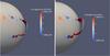 |
Fig. 8 Potential Field Source Surface (PFSS) extrapolations using magnetograms from GONG (left panel) and SDO/HMI (right panel). The line-of-sight averaged magnetic field along the line used in Fig. 3 yields ~3.5 G for the GONG and ~8 G for the SDO/HMI magnetograms, respectively. Note that the colour bar in each panel indicates the variation in magnetic field strength of the corresponding loop system. |
The phase speed of the observed transverse waves is given by the kink speed,
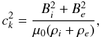 where μ0 is the permeability of a vacuum and i and e refer to loop and ambient plasma values respectively (e.g., Nakariakov & Verwichte 2005). Assuming that Bi = Be and taking the average density ⟨ ρ ⟩, an estimate for the magnetic field is given by,
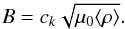 The average density is used as it reflects the fact that many oscillating structures are likely present within a single CoMP pixel (typical coronal loop widths ~200 − 1000 km, e.g., Brooks et al. 2013; Morton & McLaughlin 2013). As a result, both internal and ambient plasma will contribute to the observed emission. The estimated propagation speed and density may then be used to estimate the magnetic field, the results of which are displayed in the bottom right panel of Fig. 7. The associated uncertainties are typically ~5%, reflecting the low errors associated with propagation speed determination.
5.3. Magnetic field extrapolation
A final independent estimate was made using the magnetic field extrapolated from photospheric magnetogram observations, comparable with previous approaches (e.g., Guo et al. 2015). In this case, two Potential Field Source Surface (PFSS) extrapolations were used to estimate the magnetic field in the solar corona corresponding to the loop system impacted by the pulse (see Fig. 8). The first extrapolation shown in the left panel of Fig. 8 used a GONG magnetogram as a basis and estimated the global corona magnetic field using the finite differences method developed by Tóth et al. (2011), also used in a study concerning the magnetic structure surrounding an AR (Mandrini et al. 2014). The second extrapolation (right panel of Fig. 8) was obtained from the PFSS package within SolarSoft described by Schrijver & DeRosa (2003) using a SDO/HMI magnetogram as a basis.
Figure 8 shows that the two magnetograms initially used to extrapolate the coronal magnetic field are slightly different, as would be expected given the different sensitivity and resolution of the two instruments. This discrepancy affects the resulting extrapolated magnetic fields, so that the strength of the magnetic field along the transequatorial loop system is slightly different in both cases. The GONG (SDO/HMI) extrapolations suggest a magnetic field of ≈5 G (≈10 G) in the legs of the loop system, with the magnetic field in both cases dropping to ≈1 G at the loop-top. Along the line of sight used in Fig. 3, the extrapolations return estimates of ≈3.5 G and ≈8 G for the GONG and SDO/HMI magnetograms respectively.
6. Conclusion
Here, we have used several independent techniques to estimate the magnetic field strength within a trans-equatorial loop system following the impact of a global EUV wave-pulse. The initial impact of the wave-pulse drove a kink-mode oscillation of the loop system, allowing an estimate to be made of the magnetic field strength. This was then compared to the magnetic field strength obtained via magnetoseismology of the ubiquitous transverse waves previously observed by Tomczyk et al. (2007) and Morton et al. (2015, 2016). Finally, both sets of data-driven estimates were compared to extrapolated magnetic field measurements. All estimates were found to be broadly similar, consistent with previous results. This builds on work previously presented at the IAU Symposium on Solar and Stellar Flares and Their Effects on Planets (described by Long et al. 2016) by using multiple independent techniques including direct measurement using CoMP and EMD analysis of the CoMP Doppler oscillation to determine the magnetic field strength of the loop system.
While previous observations have shown coronal loop oscillations initially driven by the impact of a global EUV wave (e.g., Ballai et al. 2011; Guo et al. 2015), this event is unique for several reasons. The trans-equatorial loop system was located adjacent to the erupting active region, with the result that the global EUV wave-pulse was only observed to propagate southward away from the active region. The eruption was also observed by the CoMP instrument, making it one of only a handful of events observed by CoMP (cf, Tian et al. 2013). The oscillation of the loop system was only apparent in the CoMP measurements of Doppler velocity, indicating that the erupting active region was closer to the observer than the loop system along the line-of-sight.
This oscillation of the trans-equatorial loop system in CoMP Doppler velocity was identified along the loop, and was measured by fitting an exponentially decaying cosine function. It was found that while the amplitude of the oscillation decreased with height, the period and damping time were found to be comparable along the loop. This suggests that the wave-pulse initially impacted the leg of the loop, which is consistent with the large-scale nature of the loop system.
Despite the clear oscillation in CoMP Doppler velocity, no clear oscillation was observed in either the CoMP line width or the AIA intensity. However, oscillation was observed in both measurements when processed using an Empirical Mode Decomposition. This approach allowed an oscillation period and damping rate to be estimated from the line width and AIA intensity measurements, both of which are comparable to the CoMP Doppler velocity measurements, albeit with a slightly lower value. Although this suggests that the EMD approach may be beneficial for measuring oscillations in future observations, it should be noted that some component mixing was observed, which resulted in an overestimation of the oscillation frequency when fitted with a single frequency. Despite this, the signal in AIA intensity identified using the EMD analysis confirmed the kink mode nature of the oscillation.
The kink mode nature of the observed oscillation allowed an estimate to be made of the magnetic field strength within the loop system. The oscillation was measured across the loop at a range of heights and position angles, giving a mean magnetic field strength of ≈5.5 ± 1.5 G along the loop. This is comparable to the magnetic field strength of ≈1–9 G estimated using the independent magnetoseismology approach of Morton et al. (2015, 2016). It is also comparable to the extrapolated magnetic field obtained from both HMI and GONG magnetograms, suggesting that the approach is valid, albeit within the limitations previously discussed by Verwichte et al. (2013).
In addition to the oscillation of the loop system previously described, the EMD analysis may also have allowed information on the pulse itself to be discerned which is inaccessible without a time-frequency analysis. Two clear signals were identified in the CoMP line width and AIA intensity: the oscillation of the loop system and a nonlinear signal. This nonlinear signal may correspond to the global EUV wave-pulse itself, in which case it is observational confirmation of the suggestion previously made by Long et al. (2011a) that global EIT waves may be treated as a linear superposition of sinusoidal waves within a Gaussian envelope. Alternatively it may be a complex signal resulting from the interaction of the pulse and the loop system. As this set of observations is not optimal for discriminating between these possibilities, we intend to identify and further investigate the signal in future work.
Movie
Movie of Figs. 1 and 2 Access here
Acknowledgments
The authors wish to thank Lidia van Driel-Gesztelyi, Marco Stangalini, Pascal Démoulin, Cristina Mandrini, Francesco Zuccarello and Steve Tomczyk for useful discussions as well as Christian Bethge and Hui Tian for discussions on density measurements with CoMP. The authors also wish to thank the referee for their comments which helped to improve the article. D.M.L. and R.J.M. are Early Career Fellows funded by the Leverhulme Trust. D.P.S. was funded by the US Air Force Office of Scientific Research under Grant No. FA9550-14-1-0213. GV is funded by the Leverhulme Trust under Research Project Grant 2014-051. SDO/AIA data is courtesy of NASA/SDO and the AIA science team. CoMP data is courtesy of the Mauna Loa Solar Observatory, operated by the High Altitude Observatory, as part of the National Center for Atmospheric Research (NCAR). N.C.A.R. is supported by the National Science Foundation.
References
- Aschwanden, M. J., & Schrijver, C. J. 2011, ApJ, 736, 102 [NASA ADS] [CrossRef] [Google Scholar]
- Aschwanden, M. J., Fletcher, L., Schrijver, C. J., & Alexander, D. 1999, ApJ, 520, 880 [NASA ADS] [CrossRef] [Google Scholar]
- Attrill, G. D. R., Harra, L. K., van Driel-Gesztelyi, L., & Démoulin, P. 2007, ApJ, 656, L101 [NASA ADS] [CrossRef] [Google Scholar]
- Ballai, I. 2007, Sol. Phys., 246, 177 [NASA ADS] [CrossRef] [Google Scholar]
- Ballai, I., Douglas, M., & Marcu, A. 2008, A&A, 488, 1125 [NASA ADS] [CrossRef] [EDP Sciences] [Google Scholar]
- Ballai, I., Jess, D. B., & Douglas, M. 2011, A&A, 534, A13 [NASA ADS] [CrossRef] [EDP Sciences] [Google Scholar]
- Brooks, D. H., Warren, H. P., Ugarte-Urra, I., & Winebarger, A. R. 2013, ApJ, 772, L19 [NASA ADS] [CrossRef] [Google Scholar]
- Chen, P. F., Wu, S. T., Shibata, K., & Fang, C. 2002, ApJ, 572, L99 [NASA ADS] [CrossRef] [Google Scholar]
- Chen, P. F., Fang, C., & Shibata, K. 2005, ApJ, 622, 1202 [Google Scholar]
- Culhane, J. L., Harra, L. K., James, A. M., et al. 2007, Sol. Phys., 243, 19 [Google Scholar]
- Delaboudinière, J.-P., Artzner, G. E., Brunaud, J., et al. 1995, Sol. Phys., 162, 291 [NASA ADS] [CrossRef] [Google Scholar]
- Delannée, C. 2000, ApJ, 545, 512 [Google Scholar]
- Delannée, C., & Aulanier, G. 1999, Sol. Phys., 190, 107 [NASA ADS] [CrossRef] [Google Scholar]
- Delannée, C., Török, T., Aulanier, G., & Hochedez, J.-F. 2008, Sol. Phys., 247, 123 [NASA ADS] [CrossRef] [Google Scholar]
- Dere, K. P., Brueckner, G. E., Howard, R. A., et al. 1997, Sol. Phys., 175, 601 [NASA ADS] [CrossRef] [Google Scholar]
- Domingo, V., Fleck, B., & Poland, A. I. 1995, Sol. Phys., 162, 1 [NASA ADS] [CrossRef] [Google Scholar]
- Flower, D. R., & Pineau des Forets, G. 1973, A&A, 24, 181 [NASA ADS] [Google Scholar]
- Gallagher, P. T., & Long, D. M. 2011, Space Sci. Rev., 158, 365 [NASA ADS] [CrossRef] [Google Scholar]
- Gopalswamy, N., Yashiro, S., Temmer, M., et al. 2009, ApJ, 691, L123 [NASA ADS] [CrossRef] [Google Scholar]
- Grechnev, V. V., Uralov, A. M., Slemzin, V. A., et al. 2008, Sol. Phys., 253, 263 [NASA ADS] [CrossRef] [Google Scholar]
- Grechnev, V. V., Afanasyev, A. N., Uralov, A. M., et al. 2011, Sol. Phys., 273, 461 [NASA ADS] [CrossRef] [Google Scholar]
- Guo, Y., Erdélyi, R., Srivastava, A. K., et al. 2015, ApJ, 799, 151 [NASA ADS] [CrossRef] [Google Scholar]
- Handy, B. N., Acton, L. W., Kankelborg, C. C., et al. 1999, Sol. Phys., 187, 229 [NASA ADS] [CrossRef] [Google Scholar]
- Hannah, I. G., & Kontar, E. P. 2013, A&A, 553, A10 [NASA ADS] [CrossRef] [EDP Sciences] [Google Scholar]
- Harra, L. K., Williams, D. R., Wallace, A. J., et al. 2009, ApJ, 691, L99 [NASA ADS] [CrossRef] [Google Scholar]
- Huang, N. E., Shen, Z., Long, S. R., et al. 1998, Proc. Roy. Soc. London Ser. A, 454, 903 [NASA ADS] [CrossRef] [Google Scholar]
- Kaiser, M. L., Kucera, T. A., Davilla, J. M., et al. 2008, Space Sci. Rev., 136, 5 [NASA ADS] [CrossRef] [Google Scholar]
- Kienreich, I. W., Muhr, N., Veronig, A. M., et al. 2013, Sol. Phys., 286, 201 [NASA ADS] [CrossRef] [Google Scholar]
- Kwon, R.-Y., Kramar, M., Wang, T., et al. 2013, ApJ, 776, 55 [Google Scholar]
- Landi, E., DelZanna, G., Young, P. R., Dere, K. P., & Mason, H. E. 2012, ApJ, 744, 99 [NASA ADS] [CrossRef] [Google Scholar]
- Lemen, J. R., Title, A. M., Akin, D. J., et al. 2012, Sol. Phys., 275, 17 [NASA ADS] [CrossRef] [Google Scholar]
- Liu, W., & Ofman, L. 2014, Sol. Phys., 289, 3233 [NASA ADS] [CrossRef] [Google Scholar]
- Long, D. M., Gallagher, P. T., McAteer, R. T. J., & Bloomfield, D. S. 2008, ApJ, 680, L81 [Google Scholar]
- Long, D. M., Gallagher, P. T., McAteer, R. T. J., & Bloomfield, D. S. 2011a, A&A, 531, A42 [NASA ADS] [CrossRef] [EDP Sciences] [Google Scholar]
- Long, D. M., DeLuca, E. E., & Gallagher, P. T. 2011b, ApJ, 741, L21 [Google Scholar]
- Long, D. M., Williams, D. R., Régnier, S., & Harra, L. K. 2013, Sol. Phys., 288, 567 [NASA ADS] [CrossRef] [Google Scholar]
- Long, D. M., Bloomfield, D. S., Gallagher, P. T., & Pérez-Suárez, D. 2014, Sol. Phys., 66 [Google Scholar]
- Long, D. M., Baker, D., Williams, D. R., et al. 2015, ApJ, 799, 224 [NASA ADS] [CrossRef] [Google Scholar]
- Long, D. M., Pérez-Suárez, D., & Valori, G. 2016, in Solar and Stellar Flares and their Effects on Planets, eds. A. G. Kosovichev et al., Proc. IAU Symp., 320, 98 [NASA ADS] [Google Scholar]
- Long, D. M., Bloomfield, D. S., Chen, P. F., et al. 2017, Sol. Phys., 292, 7 [Google Scholar]
- Mandrini, C. H., Nuevo, F. A., Vásquez, A. M., et al. 2014, Sol. Phys., 289, 4151 [Google Scholar]
- Moreton, G. E. 1960, AJ, 65, 494 [Google Scholar]
- Moreton, G. E., & Ramsey, H. E. 1960, PASP, 72, 357 [Google Scholar]
- Moses, D., Clette, F., Delaboudinière, J.-P., et al. 1997, Sol. Phys., 175, 571 [NASA ADS] [CrossRef] [Google Scholar]
- Morgan, H., & Druckmüller, M. 2014, Sol. Phys., 289, 2945 [NASA ADS] [CrossRef] [Google Scholar]
- Morton, R. J., & McLaughlin, J. A. 2013, A&A, 553, L10 [NASA ADS] [CrossRef] [EDP Sciences] [Google Scholar]
- Morton, R. J., Tomczyk, S., & Pinto, R. 2015, Nat. Comm., 6, 7813 [Google Scholar]
- Morton, R. J., Tomczyk, S., & Pinto, R. F. 2016, ApJ, 828, 89 [NASA ADS] [CrossRef] [Google Scholar]
- Muhr, N., Veronig, A. M., Kienreich, I. W., et al. 2014, Sol. Phys., 289, 4563 [NASA ADS] [CrossRef] [Google Scholar]
- Nakariakov, V. M., & Ofman, L. 2001, A&A, 372, L53 [NASA ADS] [CrossRef] [EDP Sciences] [Google Scholar]
- Nakariakov, V. M., & Verwichte, E. 2005, Liv. Rev. Sol. Phys., 2, 65 [Google Scholar]
- Nitta, N. V., Schrijver, C. J., Title, A. M., & Liu, W. 2013, ApJ, 776, 58 [NASA ADS] [CrossRef] [Google Scholar]
- Patsourakos, S., & Vourlidas, A. 2012, Sol. Phys., 281, 187 [NASA ADS] [Google Scholar]
- Patsourakos, S., Vourlidas, A., & Stenborg, G. 2010, ApJ, 724, L188 [Google Scholar]
- Pesnell, W. D., Thompson, B. J., & Chamberlin, P. C. 2012, Sol. Phys., 275, 3 [NASA ADS] [CrossRef] [Google Scholar]
- Quek, S. T., Tua, P. S., & Wang, Q. 2003, Smart Materials and Structures, 12, 447 [CrossRef] [Google Scholar]
- Roberts, B., Edwin, P. M., & Benz, A. O. 1984, ApJ, 279, 857 [NASA ADS] [CrossRef] [Google Scholar]
- Schrijver, C. J., & DeRosa, M. L. 2003, Sol. Phys., 212, 165 [Google Scholar]
- Sedov, L. I. 1959, Similarity and Dimensional Methods in Mechanics (New York: Academic Press) [Google Scholar]
- Shen, Y., Liu, Y., Su, J., et al. 2013, ApJ, 773, L33 [NASA ADS] [CrossRef] [Google Scholar]
- Stangalini, M., Consolini, G., Berrilli, F., De Michelis, P., & Tozzi, R. 2014, A&A, 569, A102 [NASA ADS] [CrossRef] [EDP Sciences] [Google Scholar]
- Taylor, G. 1950a, Roy. Soc. London Proc. Ser. A, 201, 159 [NASA ADS] [Google Scholar]
- Taylor, G. 1950b, Roy. Soc. London Proc. Ser. A, 201, 175 [Google Scholar]
- Tian, H., Tomczyk, S., McIntosh, S. W., et al. 2013, Sol. Phys., 288, 637 [NASA ADS] [CrossRef] [Google Scholar]
- Thompson, B. J., & Myers, D. C. 2009, ApJS, 183, 225 [Google Scholar]
- Thompson, B. J., Plunkett, S. P., Gurman, J. B., et al. 1998, Geophys. Res. Lett., 25, 2465 [Google Scholar]
- Thompson, B. J., Reynolds, B., Aurass, H., et al. 2000, Sol. Phys., 193, 161 [NASA ADS] [CrossRef] [Google Scholar]
- Tomczyk, S., & McIntosh, S. W. 2009, ApJ, 697, 1384 [NASA ADS] [CrossRef] [Google Scholar]
- Tomczyk, S., McIntosh, S. W., Keil, S. L., et al. 2007, Science, 317, 1192 [NASA ADS] [CrossRef] [PubMed] [Google Scholar]
- Tomczyk, S., Card, G. L., Darnell, T., et al. 2008, Sol. Phys., 247, 411 [NASA ADS] [CrossRef] [Google Scholar]
- Tóth, G., van der Holst, B., & Huang, Z. 2011, ApJ, 732, 102 [Google Scholar]
- Uchida, Y. 1968, Sol. Phys., 4, 30 [NASA ADS] [CrossRef] [Google Scholar]
- Van Doorsselaere, T., Nakariakov, V. M., Young, P. R., & Verwichte, E. 2008a, A&A, 487, L17 [NASA ADS] [CrossRef] [EDP Sciences] [Google Scholar]
- Van Doorsselaere, T., Nakariakov, V. M., & Verwichte, E. 2008b, ApJ, 676, L73 [NASA ADS] [CrossRef] [Google Scholar]
- Veronig, A. M., Temmer, M., & Vršnak, B. 2008, ApJ, 681, L113 [Google Scholar]
- Verwichte, E., Van Doorsselaere, T., Foullon, C., & White, R. S. 2013, ApJ, 767, 16 [NASA ADS] [CrossRef] [Google Scholar]
- Vršnak, B., & Lulić, S. 2000a, Sol. Phys., 196, 157 [Google Scholar]
- Vršnak, B., & Lulić, S. 2000b, Sol. Phys., 196, 181 [NASA ADS] [CrossRef] [Google Scholar]
- Vršnak, B., & Cliver, E. W. 2008, Sol. Phys., 253, 215 [NASA ADS] [CrossRef] [Google Scholar]
- Warmuth, A. 2007, Lect. Notes Phys., 725 (Berlin: Springer Verlag), 107 [Google Scholar]
- Warmuth, A. 2015, Liv. Rev. Sol. Phys., 12, 3 [Google Scholar]
- Warmuth, A., & Mann, G. 2005, A&A, 435, 1123 [NASA ADS] [CrossRef] [EDP Sciences] [Google Scholar]
- Warmuth, A., Vršnak, B., Magdalenić, J., Hanslmeier, A., & Otruba, W. 2004a, A&A, 418, 1101 [NASA ADS] [CrossRef] [EDP Sciences] [Google Scholar]
- Warmuth, A., Vršnak, B., Magdalenić, J., Hanslmeier, A., & Otruba, W. 2004b, A&A, 418, 1117 [NASA ADS] [CrossRef] [EDP Sciences] [Google Scholar]
- West, M. J., Zhukov, A. N., Dolla, L., & Rodriguez, L. 2011, ApJ, 730, 122 [NASA ADS] [CrossRef] [Google Scholar]
- Yang, L., Zhang, J., Liu, W., Li, T., & Shen, Y. 2013, ApJ, 775, 39 [NASA ADS] [CrossRef] [Google Scholar]
- Zhukov, A. N. 2011, J. Atmospheric and Solar-Terrestrial Physics, 73, 1096 [Google Scholar]
All Figures
|
Fig. 1 Intensity image from SDO 193 Å (panel a)) and Doppler velocity from CoMP (panel b)). The dashed lines above the limb (at a height 1.09 R⊙) in both panels are used to make Fig. 3. The arc sector in the top right of panel a) shows the region used to get the density of the quiet Sun in Sect. 5.1. Note that the intensity image in panel a) has been enhanced using the Multi-scale Gaussian Normalisation technique of Morgan & Druckmüller (2014). The evolution of the 193 Å channel is shown in the left panel of the movie available online. |
| In the text | |
|
Fig. 2 Running difference images from the 193 Å passband of the eruption (panel a)) and the evolution of the wave (panel c)). The temporal evolution of the wave is shown in the right panel of the movie available online (showing the west half of the solar disk only). Panel b) shows a base-difference deprojected annulus image showing the eruption at 23:15:06 UT, with the vertical axis giving the height from Sun-centre and the horizontal axis giving the position angle clockwise from solar north (indicated by the dashed white line in panel a)). Panel d) shows a base-difference image of the temporal variation at a height of 1.09 R⊙ (indicated by the white dashed line in panel b)). The dashed white line in panel d) shows the fit to the leading edge of the propagating pulse. |
| In the text | |
|
Fig. 3 Temporal variation in CoMP Doppler velocity (panel a)) and line width (panel c)) and AIA 193 Å percentage base difference (PBD) intensity (panel e)) at a height of 1.09 R⊙ (shown by the dashed line in panels a) and b) of Fig. 1). Panels b), d) and f) show the temporal variation in Doppler velocity, line width and AIA PBD intensity along the dashed line indicated in panels a), c) and e). The oscillatory behaviour of the loop system is very clear in the Doppler motion (panels a) and b)), indicating motion to-and-from the observer, while the impact of the pulse and subsequent evacuation of plasma into the CME is apparent in the line width (panels c) and d)) and plane-of-sky AIA observations respectively (panels e) and f)), as described in the text. The solid blue line in panel b) indicates a fit to the data using the damped cosine model described in Eq. (1). |
| In the text | |
|
Fig. 4 Temporal variation in Doppler velocity at heights of 1.11, 1.12, 1.13 and 1.14 R⊙ for all polar angles (left column) along with its temporal profile measured at angles of 94°, 86°, 85° and 88° clockwise from solar north (right column). The solid blue lines in the right column indicate a fit to the data using the damped cosine model described in Eq. (1). |
| In the text | |
|
Fig. 5 Intrinsic Mode Functions derived from the time evolution of the Doppler velocity (left panels), line width (centre panels) and AIA PBD intensity (right panels), corresponding to the data in the right panels of Fig. 3. In each case the bottom panel shows the original signal (cf. Fig. 3b, d and f) with the upper panels giving the derived components. |
| In the text | |
|
Fig. 6 Hilbert Huang Transform (HHT) spectra for the Doppler velocity (left column), line width (centre column) and PBD intensity (right column) corresponding to the IMFs shown in Fig. 5. Note that only the HHT of the IMF = 3 and residual, IMF = 3 and 4, and IMF = 4 and 5 are shown in the three cases, respectively. |
| In the text | |
|
Fig. 7 The results of the magneto-seismology of propagating transverse waves. The top left panel shows the coronal loop as observed in 10 747 Å line centroid wavelength at 18:43 UT, with the measured propagation speeds of the transverse waves shown in the top right panel. The white contour over the intensity image shows the region in 10 798 Å that has adequate signal level. The lower left panel displays the estimates of plasma density from the 10 798 Å/10 747 Å ratio and the right hand panel shows the magnetic field estimate. |
| In the text | |
|
Fig. 8 Potential Field Source Surface (PFSS) extrapolations using magnetograms from GONG (left panel) and SDO/HMI (right panel). The line-of-sight averaged magnetic field along the line used in Fig. 3 yields ~3.5 G for the GONG and ~8 G for the SDO/HMI magnetograms, respectively. Note that the colour bar in each panel indicates the variation in magnetic field strength of the corresponding loop system. |
| In the text | |
Current usage metrics show cumulative count of Article Views (full-text article views including HTML views, PDF and ePub downloads, according to the available data) and Abstracts Views on Vision4Press platform.
Data correspond to usage on the plateform after 2015. The current usage metrics is available 48-96 hours after online publication and is updated daily on week days.
Initial download of the metrics may take a while.