| Issue |
A&A
Volume 603, July 2017
|
|
|---|---|---|
| Article Number | A91 | |
| Number of page(s) | 14 | |
| Section | Stellar atmospheres | |
| DOI | https://doi.org/10.1051/0004-6361/201629982 | |
| Published online | 12 July 2017 | |
The VLT-FLAMES Tarantula Survey
XXVII. Physical parameters of B-type main-sequence binary systems in the Tarantula nebula⋆,⋆⋆
1 Astrophysics Research Centre, School of Mathematics and Physics, Queen’s University Belfast, Belfast BT7 1NN, UK
2 Sub-department of Atmospheric, Oceanic and Planetary Physics, Department of Physics, University of Oxford, Oxford, OX1 3RH, UK
e-mail: ryan.garland@physics.ox.ac.uk
3 UK Astronomy Technology Centre, Royal Observatory Edinburgh, Blackford Hill, Edinburgh, EH9 3HJ, UK
4 Department of Physics and Astronomy, Hounsfield Road, University of Sheffield, S3 7RH, UK
5 Department of Physics and Astronomy, University College London, Gower Street, London WC1E 6BT, UK
6 Anton Pannenkoek Institute for Astronomy, University of Amsterdam, 1090 GE Amsterdam, The Netherlands
7 Argelander-Institut für Astronomie der Universität Bonn, Auf dem Hügel 71, 53121 Bonn, Germany
8 European Space Astronomy Centre (ESAC), Camino bajo del Castillo, s/n Urbanizacion Villafranca del Castillo, Villanueva de la Cañada, 28692 Madrid, Spain
9 King’s College London, Graduate School, Waterloo Bridge Wing, Franklin Wilkins Building, 150 Stamford Street, London SE1 9NH, UK
10 Instituut voor Sterrenkunde, Universiteit Leuven, Celestijnenlaan 200 D, 3001 Leuven, Belgium
11 Department of Physics, University of Oxford, Keble Road, Oxford OX1 3RH, UK
12 Instituto de Astrofísica de Canarias, 38200 La Laguna, Tenerife, Spain
13 Departamento de Astrofísica, Universidad de La Laguna, 38205 La Laguna, Tenerife, Spain
14 Armagh Observatory, College Hill, Armagh, BT61 9DG, UK
Received: 31 October 2016
Accepted: 10 April 2017
A spectroscopic analysis has been undertaken for the B-type multiple systems (excluding those with supergiant primaries) in the VLT-FLAMES Tarantula Survey (VFTS). Projected rotational velocities, vesini, for the primaries have been estimated using a Fourier Transform technique and confirmed by fitting rotationally broadened profiles. A subset of 33 systems with vesini ≤ 80 km s-1 have been analysed using a TLUSTY grid of model atmospheres to estimate stellar parameters and surface abundances for the primaries. The effects of a potential flux contribution from an unseen secondary have also been considered. For 20 targets it was possible to reliably estimate their effective temperatures (Teff) but for the other 13 objects it was only possible to provide a constraint of 20 000 ≤ Teff ≤ 26 000 K – the other parameters estimated for these targets will be consequently less reliable. The estimated stellar properties are compared with evolutionary models and are generally consistent with their membership of 30 Doradus, while the nature of the secondaries of 3 SB2 system is discussed. A comparison with a sample of single stars with vesini ≤ 80 km s-1 obtained from the VFTS and analysed with the same techniques implies that the atmospheric parameters and nitrogen abundances of the two samples are similar. However, the binary sample may have a lack of primaries with significant nitrogen enhancements, which would be consistent with them having low rotational velocities and having effectively evolved as single stars without significant rotational mixing. This result, which may be actually a consequence of the limitations of the pathfinder investigation presented in this paper, should be considered as a motivation for spectroscopic abundance analysis of large samples of binary stars, with high quality observational data.
Key words: stars: early-type / stars: abundances / binaries: spectroscopic / ISM: individual objects: Tarantula Nebula (except planetary nebulae)
Based on observations collected at the European Organisation for Astronomical Research in the Southern Hemisphere under ESO programme 182.D-0222.
Tables 6 and 7 are only available at the CDS via anonymous ftp to cdsarc.u-strasbg.fr (130.79.128.5) or via http://cdsarc.u-strasbg.fr/viz-bin/qcat?J/A+A/603/A91
© ESO, 2017
1. Introduction
The quantitative analysis of the spectra of early-type stars provides a powerful tool for understanding their formation and evolution. With the development of both observational and theoretical techniques is has been possible to move from the pioneering analyses of single bright targets in our Galaxy (see, for example, Unsöld 1942) to large-scale surveys in external galaxies (see, for example, Evans et al. 2008, 2011b). Currently quantitative spectroscopy is possible to a distance of several megaparsecs (e.g. Kudritzki et al. 2016), with the next generation of ground-based telescopes expected to reach beyond 10 Mpc (Evans et al. 2011a).
Complementing these observational advances has been an improved understanding of how early-type stars evolve (see, for example, Maeder 2009; Langer 2012). This includes the importance of rotation in both the evolution of the star (Heger et al. 2000; Hirschi et al. 2004) and in the mixing of nucleosynthesised material to the stellar surface (Maeder 1987; Heger & Langer 2000; Frischknecht et al. 2010). Additionally, mass loss can be significant, particularly for more luminous stars and in metal-rich environments (Puls et al. 2008; Mokiem et al. 2007) and this can effect their evolution (Chiosi & Maeder 1986). More recently it has been recognised that magnetic fields (Donati & Landstreet 2009) can affect the internal structure and rotation profile, which in turn can affect chemical mixing. For example, Petermann et al. (2015) discuss the effects of magnetic fields on the mixing between a stellar core and its envelope. Additionally stellar oscillation modes or internal gravity waves (Aerts et al. 2014) could be important. These developments have allowed the generation of extensive grids of evolutionary models (see, for example, Brott et al. 2011a; Ekström et al. 2012; Georgy et al. 2013), which have been used to synthesize stellar populations for comparison with the results from large-scale surveys (Brott et al. 2011b; Grin et al. 2016).
Most quantitative analyses of stellar spectroscopy have implicitly or explicitly assumed that their targets have evolved as single stars. However, it has recently become apparent that most early-type stars are in binary systems (Mason et al. 2009). For example, Sana et al. (2012) estimated an intrinsic binary fraction of 0.69 ± 0.09 for Galactic O-type systems, with a strong preference for closely bound systems. Other Galactic studies include Kobulnicky et al. (2014, binary fraction with periods less than 5000 days of approximately 0.55), Mahy et al. (2009, lower limit of 0.17 for O-type systems), Mahy et al. (2013, 0− and Pfuhl et al. (2014,  . In the Large Magellanic Cloud (LMC), Sana et al. (2013) estimated a fraction of 0.51 ± 0.04 for the O-type stellar population of the 30 Doradus regio observed in the VLT-FLAMES Tarantula survey (VFTS; Evans et al. 2011b, hereinafter Paper I). Additionally Dunstall et al. (2015) inferred a similar high fraction (0.58 ± 0.11) for the B-type stellar population in the same survey.
The above estimates are for the current intrinsic fraction of binary systems. Theoretical simulations (de Mink et al. 2014) imply that a significant fraction of massive stellar systems (typically ~8%) might be the products of stellar mergers. In turn this would imply an even higher fraction (~19%) of currently single stars have previously been in a binary system. For example, de Mink et al. (2014) discuss the possibility that the higher fraction of binaries found in young Galactic O-type stars (Sana et al. 2012) than in the VFTS sample (Sana et al. 2013) might be due to stellar evolution and binary interactions having modified the intrinsic binary fraction of the latter. Although there remains some uncertainty in the intrinsic binary fractions (as a function of age and metallicity) and in the relative importance of the diverse evolutionary channels available to binary systems, it is clear that binarity must play a central role in the evolution of early-type stars.
Given the above, it may appear surprising that there have been few quantitative analyses of the spectra of early-type binaries (see Sect. 4.4). This probably reflects the difficulty of identifying and observing binary systems and also the additional complexity of allowing for the flux contributions of the secondaries. Although methods exist for disentangling the components in high-quality spectroscopy of SB2 systems (see, for example, González & Levato 2006; Howarth et al. 2015), these are not readily applicable to SB1 systems or to spectroscopy with moderate signal-to-noise ratios.
Here we present what we believe to be the first model-atmosphere analysis of a significant sample of B-type spectroscopic binaries that are not supergiants. These were taken from the binary sample identified in the VFTS (Dunstall et al. 2015) but were limited to those stars with relatively narrow metal-absorption lines in order to facilitate their analysis. We emphasize that, given the complexities of modelling the spectra of binary systems and the biases in our sample, this should be considered as a pathfinder analysis, although we believe that the scientific results will still be useful in constraining theoretical models.
The observational data are discussed in Sect. 2 and the analysis in Sect. 3. Results are discussed in Sect. 4, which contains a comparison with a sample of apparently single stars from the same survey.
2. Observations
As described in Paper I and McEvoy et al. (2015), the Medusa mode of FLAMES (Pasquini et al. 2002) was used to collect the VFTS data. This uses fibres to observe up to 130 sky positions simultaneously with the Giraffe spectrograph. FLAMES has a corrected field-of-view of 25′ and hence with one telescope pointing, we were able to observe stars both in the local environs of 30 Doradus as well as in the main body of the H II region. Nine Medusa fibre configurations (Fields “A” to “I” with an identical field centre) were employed to obtain our sample of approximately 800 stellar objects. Two standard Giraffe settings were used, viz. LR02 (wavelength range from 3960 to 4564 Å at a spectral resolving power of R ~ 7000) and LR03 (4499−5071Å, R ~ 8500). Details of target selection, observations, and data reduction have been given in Paper I.
2.1. Sample selection
The B-type candidates identified in Paper I and subsequently classified by Evans et al. (2015) were analysed by Dunstall et al. (2015) using a cross-correlation technique. Eleven supergiant and 90 lower-luminosity targets with radial-velocity variations that were both statistically significant and had amplitudes larger than 16 km s-1 were classified as binary1. A further 17 supergiants and 23 lower-luminosity targets were classified as “RV variables” by Dunstall et al. (2015); we exclude those targets as their radial-velocity variations may not be due to binarity.
The supergiants have been discussed by McEvoy et al. (2015) and will not be considered further here. Projected rotational velocities (vesini) have been estimated for the primaries of the remaining 90 binary candidates, using similar techniques to those adopted by Dufton et al. (2013). Details of the methodology are provided in Appendix A, whilst the estimates are given in Tables 6 and 7 (only available at the CDS). These have a similar format to the online Tables 3 and 4 in Dufton et al. (2013).
A quantitative analysis of all these binaries including those with large projected rotational velocities would be possible in principle. However, because of the moderate signal-to-noise ratios (S/N) in our spectroscopy, the atmospheric parameters would be poorly constrained (in particular, effective temperatures – see Sect. 3.2). In turn this would lead to nitrogen abundance estimates that had little diagnostic value. Hence for the purposes of this paper we have limited our sample to the subset of binaries with relatively small projected rotational velocities.
The thirty-seven binaries with projected equatorial rotational velocities vesini ≤ 80 km s-1 are listed in Table 1, along with their spectral types (Evans et al. 2015; Walborn et al. 2014) and typical S/Ns and observed range of radial velocity variations, Δvr (Evans et al. 2015). As the LR02 wavelength region 4200–4250 Å should not contain strong spectral lines, our S/Ns were estimated from that region. We should consider these as lower limits, however, as weak absorptions lines could have an affect (especially for higher S/Ns). S/Ns for the LR03 region were normally similar to or slightly smaller than those for the LR02 region (see, for example, McEvoy et al. 2015, for a comparison of S/Ns in the two spectral regions). The estimates of Δvr will be related to the amplitude of the primary’s radial velocity variations (depending on the sampling of the orbit they will be similar to but generally lower than twice the amplitude) and hence provide insight into whether the systems are tightly bound.
Four targets proved resistant to quantitative analysis (see Sect. 3.1), leaving 33 for which a detailed study could be undertaken. For the most part, these are single-lined (SB1) systems as far as our data are concerned; only three targets, discussed in Sect. 4.1, show any direct evidence for a secondary spectrum.
Spectral classifications (from Evans et al. 2015), estimated projected rotational velocity (vesini), typical signal-to-noise ratios (S/N) for the LR02 region (which have been rounded to the nearest multiple of five) and observed ranges of radial velocity variations of the primary, Δvr.
2.2. Data preparation
Data reduction followed the procedures discussed in Evans et al. (2011b) and Dufton et al. (2013). Because of the radial-velocity variations between epochs, care had to be taken when combining exposures. We undertook numerical experiments (discussed in Appendix A) to estimate the maximum range (Δvr) in radial-velocity measurements before the estimation of the projected rotational velocity became compromised. For slowly rotating targets, this was found to occur at Δvr ≃ 30 km s-1, and this should also be an appropriate range for a model-atmosphere analysis. Hence for targets with Δvr ≤ 30 km s-1 we combined all usable exposures for the LR02 spectra, without applying any radial-velocity shifts, using either a median or weighted σ-clipping algorithm. The two methods gave final spectra that were effectively indistinguishable. Using only exposures from a single epoch (with effectively constant radial velocity), gave comparable but lower S/N ratio results.
For those stars with greater values of Δvr most of the treatment was the same, except that either (i) spectra were shifted to allow for radial-velocity variations prior to being combined, and/or (ii) spectra from the highest S/N ratio LR02 epoch and additional epochs with radial velocities within ±15 km s-1 were combined. The latter procedure minimised the effects of nebular contamination, whilst the former led to higher S/Ns.
The time cadence for the LR03 exposures are listed in Tables A.1 and A.2 in the appendix of Paper I. For five of the Medusa fields all the exposures were taken within a period of 3 h, whilst for two other fields the spectroscopy was obtained on consecutive nights. For Field F, there was an additional observation separated by 55 days from the other six exposures but this exposure was not included in the reduction. Hence for these eight fields, simply combining exposures should be adequate, especially as no significant radial-velocity shifts (i.e., greater than 30 km s-1) were observed in LR02 exposures taken on the same or consecutive nights.
For Field I (containing eight targets: VFTS 017, 018, 278, 534, 575, 742, 850, 874), one set of LR03 exposures was separated from the others by 8 days. One target was not analysed (VFTS 278; see Sect. 3.1) but for the other seven targets the individual co-added spectra for the two epochs were cross-correlated. The wavelength region 4530–4720 Å was selected, as this contains relatively strong metal and helium absorption lines. The cross-correlations implied velocity shifts of less than 30 km s-1 and hence the individual exposures for these targets were again combined without any wavelength shifts.
3. Model-atmosphere analyses
3.1. Methodology
We employed model-atmosphere grids calculated with the tlusty and synspec codes (Hubeny 1988; Hubeny & Lanz 1995; Hubeny et al. 1998; Lanz & Hubeny 2007). They cover a range of effective temperature, 10 000 K ≤ Teff ≤ 35 000 K in steps of typically 1 500 K. Logarithmic gravities (in cm s-2) range from 4.5 dex down to the Eddington limit in steps of 0.25 dex, and microturbulences are from 0−30 km s-1 in steps of 5 km s-1. As discussed in Ryans et al. (2003) and Dufton et al. (2005), equivalent widths and line profiles interpolated within these grids are in good agreement with those calculated explicitly at the relevant atmospheric parameters.
These codes adopt the “classical” non-LTE assumptions, i.e. plane-parallel atmospheres and that the optical spectrum is unaffected by winds. As the targets considered here have luminosity classes III−V, such an approach should provide reliable results. These models assume a normal helium to hydrogen ratio (0.1 by number of atoms). The validity of this will be considered in Sect. 4.4.1. Grids have been calculated for a range of metallicities (see Ryans et al. 2003; Dufton et al. 2005 for details) with that for an LMC metallicity being used here.
For four targets (VFTS 097, 240, 278, 305), the Si iii spectra could not be reliably measured, thereby precluding estimation of the microturbulence (and also, when the He ii spectrum was absent, the effective temperature); these stars were excluded from the analysis. Another 13 targets had no observable Si ii, Si iv or He ii features in their spectra, leading to uncertainties in their effective-temperature estimates of more than ±2000 K (see Sect. 3.2 for details of methodology). These were initially excluded from our analysis on the basis that their atmospheric parameters (and hence nitrogen abundances) would be unreliable. However, the N ii lines have a maximum strength at the atmospheric parameters appropriate to these stars. This leads to the nitrogen abundance being relatively insensitive to the choice of atmospheric parameters. Hence these stars have been analysed using a modified methodology as discussed in Sect. 3.7.
For our targets, there will be an indeterminate flux contribution from the fainter secondary. To investigate the possible effects of this on our analysis, we assume that the secondary contributes 20% of the light via a featureless continuum, just as in McEvoy et al. (2015). We have chosen this value as contributions larger than this should become apparent in the secondary spectrum (but see the discussion in Sect. 4.1). A simple continuum was adopted for convenience and also because structure in the secondary spectrum (e.g. in the Balmer lines) would normally mitigate its effect. This analysis used the same methodology to that discussed below apart from the equivalent widths and hydrogen and helium line profiles having been rescaled; this approach was used previously by McEvoy et al. (2015), Dunstall et al. (2011), where more details can be found.
Due to the interdependence of the estimation of the effective temperature, surface gravity, microturbulence, and chemical abundances, an iterative process was adopted as discussed below.
3.2. Effective temperature
Effective temperatures (Teff) were initially constrained by the silicon ionisation balance, using microturbulence estimates from the absolute silicon abundance (method 2 discussed in Sect. 3.4). The equivalent widths of the Si iii triplet (4552, 4567, 4574 Å) were used in conjunction with those of either a Si iv line (4116Å) for the hotter systems, or a Si ii doublet (4128, 4130 Å) for the cooler ones. For some systems, neither the Si ii nor the Si iv lines were observable; in these cases, upper limits were set on their equivalent widths, allowing limits for the effective temperature to be estimated. Stars, where the uncertainty in the Teff estimates was greater than ±2000 K, were excluded from this analysis but are discussed further in Sect. 3.7.
Where He ii lines were present in the spectrum, two independent effective temperature estimates were made from fitting the line profiles of the features at 4541 and 4686 Å (with the theoretical profiles being convolved with the instrumental profile and with a rotational broadening function), assuming gravities estimated from the hydrogen line profiles (see Sect. 3.3) and a normal helium to hydrogen abundance. The latter assumption is considered further in Sect. 4.4.1. All the effective temperature estimates are summarised in Table 2 for the assumption that the secondary contributed no flux; the estimates assuming that the secondary contributed 20% of the flux were generally higher by 500–1000 K, as can be seen from Table 3.
Generally the estimates from the silicon and helium spectra were in good agreement, with the difference being 1000 K or less (see Table 2). This is consistent with the S/Ns of our spectroscopy (see Table 1), which lead to formal uncertainties in our equivalent widths estimates of typically less than 10%. We have therefore adopted a stochastic uncertainty in our effective-temperature estimates of ±1000 K.
Estimates of the atmospheric parameters for the primaries assuming no secondary flux contribution.
Adopted estimates for the projected rotational velocity (vesini), atmospheric parameters, silicon, magnesium and nitrogen abundance estimates.
3.3. Surface gravity
The observed hydrogen Balmer lines profiles, Hγ and Hδ, were compared to theoretical profiles (again convolved to allow for the instrumental profile and stellar rotation) in order to estimate the logarithmic surface gravities (log g; cm s-2); further details can be found in, for example, McEvoy et al. (2015). These estimates are summarised in Table 2 for the assumption that the secondary contributed no flux; the estimates assuming that the secondary contributed 20% of the flux are larger by between 0.1–0.3 dex (mainly due to the observed hydrogen line profiles being deeper) as can be seen from Table 3.
Estimates derived from the Hγ and Hδ lines generally agreed to ±0.1 dex. Factoring in other uncertainties, such as normalisation errors and possible errors in the line broadening theory, a conservative error estimate of ±0.2 dex has been adopted (note that the estimates are quoted in the tables to the nearest 0.05 dex, i.e. two significant figures, in order to illustrate the effects of the secondary flux contribution).
3.4. Microturbulence
By eliminating any systematic dependence of abundance estimates on line strength, we can estimate the microturbulent velocities (vt). To do this, we used the equivalent widths of the Si iii triplet (4552, 4567 and 4574 Å) because it is present in almost all of our spectra. All three lines are from one multiplet, which has the advantages that their relative oscillator strengths should be reliable, whilst non-LTE effects should be similar for each line. The only other choice for estimating the microturbulence, given our wavelength coverage, would have been to use the rich O ii spectra. However as discussed by Simón-Díaz et al. (2006) and Simón-Díaz (2010), this approach has several complications. Firstly many of the lines are blended, leading Simón-Díaz et al. (2006) to reject over half the features they identified. Secondly, errors in the adopted oscillator strengths or in the non-LTE effects for different multiplets can lead to systematic errors. A third difficulty specific to our observational dataset was that the O ii spectrum was weak in our coolest targets and was not therefore a sensitive diagnostic for the microturbulence.
Our methodology is illustrated in Fig. 1 for VFTS 225. As can be seen the slope of the least squares fit of the abundance estimates against equivalent widths is relatively insensitive to the choice of microturbulence. Therefore errors in the equivalent widths estimates can lead to significant errors in the estimation of the microturbulence, especially when the lines lie close to the linear part of the curve of growth (see, McEvoy et al. 2015; Dufton et al. 2005; Hunter et al. 2007, for more details). The method also requires that all three lines be observed reliably, which was not always the case with the current dataset. Additionally, large microturbulence values were obtained for VFTS 534 and VFTS 850, which appeared inconsistent with their derived gravities.
Therefore the microturbulence estimates were also obtained by ensuring that the silicon abundance is consistent with the LMC’s metallicity, since this element should not be significantly affected by nucleosynthesis in our targets (see, for example, Brott et al. 2011a). A value of 7.20 dex was adopted as found by Hunter et al. (2007) using similar analysis methods and observational data to those conducted here. Previous investigations of early-type stars in the LMC have found similar values, with for example Korn et al. (2002, 2005) finding respectively 7.10 ± 0.07 dex in 4 narrow lined (near) main sequence targets and 7.07 dex (with uncertainties in the individual measurements of ±0.3 dex) for 3 broad lined targets.
To investigate the sensitivity of our estimates to the adopted silicon abundance, we considered the effect of reducing our adopted silicon abundance to 7.1 dex. This led to a typical increase of 1 km s-1with a maximum increase of less than 2 km s-1. Additionally Fig. 1 confirms that absolute silicon abundance estimates are sensitive to the choice of the microturbulence (the silicon abundance estimate changing from approximately 7.7 dex to 7.2 dex as the microturbulence is increased from 1 to 5 km s-1), making this potentially a reliable method for estimating this quantity.
Estimates using the two methodologies are summarised in Table 2 for the assumption that the secondary contributed no flux; the estimates assuming that the secondary contributed 20% of the flux are generally larger by 2–5 km s-1 as can be seen from Table 3.
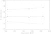 |
Fig. 1 An example of the estimation of the microturbulent velocity using the relative strengths of three Si iii lines in VFTS 225. Abundances estimates are shown for vt = 1 (triangles), 3 (stars) and 5 (crosses) km s-1, together with linear least square fits. |
Some systems were found to have a maximum silicon abundance (obtained at vt = 0 km s-1) below the adopted LMC value; furthermore, removing the variation of the abundance estimates with line strength was not always possible. These effects were mitigated by allowing a flux contribution from a secondary (see Table 3). However, both McEvoy et al. (2015) and Hunter et al. (2007) found similar effects for a number of their (presumably single) targets, with the latter discussing possible causes in some detail. In these instances, we have assumed the best-estimate microturbulence (i.e., zero).
For other targets we adopted an equivalent-width uncertainty of ±20%, normally translating to variations of up to ~5 km s-1 for both methods. Such uncertainties are consistent with the differences between the estimates using the two methodologies. Only in three cases do these differ by more than 5 km s-1 and in two of these the estimates from relative strength of the Si iii multiplet (method 1 in Table 2) appear inconsistent with the relatively high surface-gravity estimates. Hence a reasonable estimate for the uncertainty in the microturbulence estimates is ±5 km s-1.
3.5. Adopted atmospheric parameters
Table 3 summarises the adopted atmospheric parameters. The parameters are provided for the two different assumptions concerning the secondary flux contribution, viz. the primary star supplies all the observed radiative flux or that 20% of the continuum flux is from the secondary. Microturbulence estimates were from the requirement of a normal silicon abundance (method 2 in Table 2).
Magnesium abundances could be independently estimated from the equivalent width of the Mg ii doublet at 4481 Å. This element should not be affected by nucleosynthesis in (near) main-sequence stars. Hence it could be used to validate our adopted atmospheric parameters by comparing estimated abundances to the baseline LMC value (7.05 dex, as found by Hunter et al. 2007).
The mean (and standard deviations) of these magnesium abundance estimates was 6.95 ± 0.15 dex (no secondary flux contribution) and 7.08 ± 0.15 dex (20% secondary flux contribution). These are both in reasonable agreement with the baseline LMC abundance and indeed are consistent with the secondary flux contributions being within the range considered.
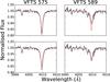 |
Fig. 2 Comparison of observed and theoretical spectra for the region near the N ii line at 3995 Å. VFTS 575 and VFTS 589 are shown to the left and right respectively. The upper and lower panels have a 0% and 20% (with the theoretical spectra being scaled) contribution from the secondary, |
3.6. Nitrogen abundances
The singlet transition at 3995 Å is normally the strongest N ii line in the LR02 and LR03 spectral regions and appears unblended (see, for example Hunter et al. 2007; McEvoy et al. 2015). Therefore estimates of its equivalent width together with a curve of growth approach were used as our primary estimator of nitrogen abundances. Surprisingly this transition was only observable in five of our systems; by contrast it was observed in approximately 50% of the equivalent single-star sample analysed by Dufton et al. (in prep.). For all of the other B-type binaries, we set an upper limit on the equivalent width using their methodology. Briefly, the equivalent widths of weak metal absorption lines were measured in VFTS spectra with different S/Ns and projected rotational velocities. These were then used to infer the upper limit of the N ii line in a binary spectrum with a given S/N ratio and projected rotational velocity.
Three of the five systems where the N ii 3995 Å line was observed also showed the N ii line at 4630 Å (other weaker components of this triplet-triplet multiplet could not be identified). VFTS 575 and VFTS 850 yielded nitrogen abundance estimates which agreed to within 0.1 dex, while VFTS 723 agreed to within 0.3 dex.
Estimates and upper limits of the chemical abundances are also affected by the errors in the atmospheric parameters. For further discussion of this, see Hunter et al. (2007) and Fraser et al. (2010). As in McEvoy et al. (2015), we conservatively adopt a typical uncertainty of 0.2–0.3 dex, which does not include any systematic errors inherent in the adopted models or the secondary flux contribution.
We validated these nitrogen abundance estimates by extracting theoretical spectra from our grid using the parameters in Table 3. We have considered both a 0% and 20% contribution from the secondary, with for the latter the theoretical spectrum being scaled. In general there was a good agreement between the theoretical (convolved to allow for instrumental and rotational broadening) and observed spectra and Fig. 2 shows some examples. For two systems (VFTS 534 and 662), the comparison indicated that their maximum nitrogen estimates could be up to 0.1–0.2 dex larger than those listed in Table 3.
Figure 2 also shows the He i line at 4009 Å. Assuming a normal helium abundance, this can be used as a further check on the atmospheric parameters. For VFTS 575, good agreement between theory and observation is found with a small secondary flux contribution, whilst for VFTS 589 a significant contribution is implied (this star was classified as SB2 and is discussed further in Sect. 4.1).
This consistency check was also carried out for the other eighteen targets and generally good agreement was found between theory and observation. An attempt was also made to characterize the amount of secondary contamination and the targets have been divided into three groups, viz., those where the contamination appeared small, those where the secondary flux contamination appeared to be approximately 20% and those where the contamination lay between 0 and 20%. For some stars, the comparison was complicated by there being evidence of nebular emission in the centre of the He i lines that had not been totally removed by the sky subtraction (due to the sky fibres being spatially separated from the target fibres – see Paper I for more details). This was particularly noticeable for VFTS 359 and VFTS 662, which were therefore excluded from this comparison. Five stars (VFTS 033, 299, 324, 665, 888) appeared to have only a small secondary flux contribution, 4 stars (VFTS 195, 204, 351, 686) had a contribution near the 20% level and 7 stars (VFTS 017, 179, 225, 534, 723, 799, 850) had contributions between 0 and 20%. It is encouraging that VFTS 686, which had been classified as SB2 showed a significant secondary flux contribution.
The comparison described above was only used as a consistency check and no attempt was made to estimate secondary flux contributions for individual systems. This was because uncertainties both observational (e.g. possible nebular emission) and in the estimated vesini and atmospheric parameters would have led to significant uncertainties. Rather we have presented nitrogen abundance estimates in Table 3 for the two representative cases (viz. seconary flux contributions of 0% and 20%) that were used to estimate the atmospheric parameters.
3.7. Targets with significant uncertainties in Teff
As discussed in Sect. 3.1, there were 13 targets with observed spectra which had neither observable lines from two ionization stages of silicon nor observable He ii profiles. In these cases, it was not possible to obtain reliable effective-temperature estimates and they were excluded from the analysis outlined in Sects. 3.1 to 3.6.
Failure to observe either the Si ii or Si iv features implied that both spectra are relatively weak. This will normally occur when they have a similar strength. The corresponding effective temperature will depend on both the adopted gravity and microturbulence. However, for the typical gravities and microturbulences found in our sample (see Table 3), it is approximately 23 000 K.
This effective temperature corresponds to that for the maximum strength of the N ii spectra. As the differential of nitrogen abundance with effective temperature is then zero, this leads to such estimates being relatively insensitive to the effective temperature. Additionally for a given observed hydrogen profile, an increase in the adopted effective temperature leads to an increase in the estimated gravity (corresponding to approximately 0.1 dex in log g for a change of 1000 K in Teff). This decreases the sensitivity of the degree of nitrogen ionization (given in LTE by the Saha equation) to changes in effective temperature. In turn this further reduces the sensitivity of the strength of the N ii lines to changes in the atmospheric parameters.
For example at (Teff, log g, vt) of (23 000, 4.0, 0), an equivalent width of 50 mÅ for the N ii 3995 Å line implies a nitrogen abundance estimate of 7.16 dex. For atmospheric parameters of (26 000, 4.3, 0) and (20 000, 3.7, 0), the estimates become 7.19 dex and 7.46 dex respectively, leading to a range of approximately 0.3 dex in nitrogen abundance estimates for an effective-temperature uncertainty of ±3000 K.
We have therefore analysed these 13 targets assuming an effective temperature of 23 000 K. For a given target, the error in the effective-temperature estimate will depend on the S/N ratio of the spectroscopy and the other atmospheric parameters. However, for effective temperatures higher than 26 000 K, the He ii spectra would normally become observable, whilst for an effective temperature of less than 20 000 K, the Si ii spectra become relatively strong (for example at Teff = 20 000 K and log g = 4.0 dex, the Si ii line at 4131 Å has predicted equivalent widths of approximately 35 and 50 mÅ for microturbulent velocities of 0 and 5 km s-1 respectively and an LMC silicon abundance).
Nitrogen abundance estimates and projected rotational velocities for targets for which a reliable effective-temperature estimate could not be obtained.
This effective-temperature range is consistent with 8 out of 13 of our targets having a spectral types of B1.5 or B2, for which the LMC effective-temperature calibration of Trundle et al. (2007) implies effective temperatures of between 21 700 and 25 700 K for luminosity classes III to V. Five of our targets have earlier spectral types and we have therefore searched for evidence of He ii features in their observed spectra. For all five stars, no evidence was found for the line at 4541 Å, whilst for two stars (VFTS 342 and 719), the line at 4686 Å was also not seen. Comparison with theoretical spectra then implied an effective temperature of less than 26 000 K for these two stars.
For two other stars (VFTS 162 and 501), there was marginal evidence for a feature at 4686 Å and fitting this (with an appropriate gravity deduced from the hydrogen lines) implied an effective temperature of approximately 26 000 K. For the final target, VFTS 520, the He ii feature at 4686 Å was more convincing implying an effective-temperature estimate of 26 500 K. Hence although not a formal error estimate, this range of effective temperatures (20 000 to 26 000 K) should be sufficient for most of our targets.
For each target, gravities could then be estimated for this range of effective temperatures, leading to nitrogen abundance estimates. These are summarised in Table 4 (for an assumed zero microturbulence) and we note that where:
-
1.
a range of nitrogen abundance estimates is given, this explicitlyincludes the uncertainty in effective temperature (and hence thegravity). The adoption of a larger microturbulence (e.g.5 km s-1) would lead to adecrease in these estimates by typically less than0.1 dex;
-
2.
an upper limit for the nitrogen abundance is given, this corresponds to the largest estimate found within our range of effective temperatures (and corresponding gravities). The adoption of a larger microturbulence (e.g. 5 km s-1) would again lead to a small decrease in these upper limits.
In summary, the analysis of these targets is less sophisticated as befits the uncertainties in estimating their effective temperatures. The nitrogen abundance estimates should therefore be treated with some caution but they provide a useful supplement to those given in Table 3. As for the other targets, we would expect that inclusion of a contribution from the unseen secondary would again lead to an increase in the estimated nitrogen abundances of approximately 0.2 dex.
4. Discussion
4.1. Double-lined spectroscopic binaries
Three of our binaries (VFTS 240, 520 and 589) were classified by Evans et al. (2015) as either SB2? or SB2. VFTS 240 was excluded from the present study due to the poor quality of its spectroscopy (Sect. 3.1). During our model-atmosphere analysis, evidence was found for a secondary spectrum in VFTS 686. We discuss these stars in more detail below:
-
VFTS 520: this was classified asB1: V (SB2?) by Evanset al. (2015) and inspection of theLR02 spectra showed evidence of a secondary in theHe i lines. As the secondary would appear to befainter this would be consistent with it having a main-sequenceearly- to mid-B spectral type.
-
VFTS 589: this was classified as B0.5 V (SB2?) by Evans et al. (2015) and in this case evidence for a secondary was apparent in its LR03 Si iii spectrum, where all the exposures were obtained at a single epoch. By contrast no evidence for a secondary was found in combined subsets of LR02 exposures obtained at a given epoch.
For all three Si iii lines near 4560 Å, a narrow absorption feature was found at approximately 1.4 Å to the red of the absorption line from the primary. Both components have a similar width (FWHM ≃ 0.87 Å and 0.89 Å for the secondary and primary, respectively), implying that the projected rotational velocity of the secondary was also ≤40 km s-1. The equivalent widths of the secondary components were approximately 50% of those of the primary. Assuming that the equivalents widths in the individual spectra were the same would then imply a flux ratio of two or a secondary flux contribution of 33%.
Similar features are present in the O ii doublet near 4593 Å in the LR03 spectral region with strengths of approximately 25% of the primary components, implying (making the same assumption as for the silicon lines) a flux ratio of four or a secondary contribution of 20%. Additionally the He i line at 4713 Å appears to have two components although there is significant contamination from nebula emission.
For the effective temperature estimated for the primary (see Table 3), the Si iii equivalent widths increase with decreasing effective temperature, whilst those of O ii decrease. The relative strengths of the binary components in the silicon and oxygen spectra would then suggest that the secondary is a main-sequence star of slightly later type than the primary. In turn this would then imply a flux contamination from the secondary of approximately 25%.
The LR03 spectral range lies close to that of the B photometric band. Assuming, for example, that the secondary had a spectral type of B1.5 V, the spectral type versus magnitude calibrations of Walborn (1972) and Pecaut & Mamajek (2013) would imply a B-magnitude difference of 0.8−0.9 and a secondary flux contribution of approximately 30%, in reasonable agreement with that estimated above. Finally we note that the upper limits for the projected rotational velocities of both components would be consistent with their rotational periods being synchronised to the orbital period.
VFTS 686:Evans et al. (2015) classified this target as a single-lined spectroscopic binary with a B0.7 III spectral type. During the model-atmosphere analysis, the presence of a secondary component was identified in the LR03 combined spectrum. As for VFTS 589, no evidence for a secondary was found in combined subsets of LR02 exposures obtained at different epochs.
The secondary was identified in the LR03 spectrum by broad, shallow components (FWHM ≃ 2.8Å) that lay approximately 1.7Å to the red of those of the narrow-lined primary. Gaussian profiles were fitted to the absorption lines of the Si iii multiplet near 4560 Å and O ii doublet near 4593 Å, together with the He i line at 4713 Å. The equivalents widths of the secondary were approximately 50% of those of the primary, although there was considerable scatter, at least in part due to the secondary components having very small central depth (~1−2%).
The use of a Gaussian profile to fit the broad (presumably rotationally dominated) profiles of the secondary may not be appropriate, Therefore we have repeated the fitting process assuming rotational broadened profiles. This led to broadly similar results but also provided estimates of the projected rotational velocity, vesini, of the secondary that were in the range 160−210 km s-1.
Because of the difficulty of measuring the spectra of the secondary, it is not possible to come to any definitive conclusions about its nature. Possibilities include that it might have a similar spectral type to the primary but a lower luminosity class, e.g. B0.7 V or that it might have a slightly later spectral type. However, the nature of its spectrum would imply that it is has an early-B spectral type, whilst it is not possible that the rotational periods of both components are synchronised to the orbital period.
The identification of these double-lined spectroscopic binaries provides an insight into our choice of a 20% secondary flux contribution when preparing Table 3. The results for VFTS 589 imply that narrow-lined secondaries should be identified (subject to them having a significantly different radial velocity to that of the primary at the time of observation) if they contribute more than 20% of the continuum flux. By contrast a rapidly rotating secondary might not be identified at such flux levels. Hence it is important that the results presented in Table 3 are considered as representative of the consequences of an unseen secondary and are not considered as a firm upper limit.
4.2. Effective temperature and surface gravity
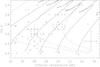 |
Fig. 3 Gravity estimates plotted against effective-temperature estimates for our binary sample listed in Table 3 (triangles), together with representative error bars. Also shown is the single-star sample discussed in Sect. 4.4.2 (crosses – some targets have been moved slightly in effective temperature or gravity in order to improve clarity). Evolutionary models (solid lines) of Brott et al. (2011a) are shown for zero initial rotational velocity together with the initial mass (in units of the solar mass). Isochrones (dashed lines) are shown for ages of 5, 10 and 20 Myr. |
Figure 3 shows the estimated effective temperatures and gravities (assuming zero flux contribution from the secondary) for our binary targets for which a full analysis was undertaken. The targets discussed in Sect. 3.7 and summarised in Table 4 have not been included due to the uncertainty in their effective temperatures. Also shown in Fig. 3 are an equivalent sample of presumed single targets from the VFTS analysed by Dufton et al. (in prep.). Both analyses used a similar methodology and hence the estimates should be comparable. However, it should be noted that although designated as “single”, the sample of Dufton et al. (in prep.) may also contain some binary systems. As discussed by Dunstall et al. (2015) and Sana et al. (2013), these will be weighted towards long-period systems which may have evolved as if they were single.
Also shown are the evolutionary tracks and isochrones of Brott et al. (2011a) for effectively zero initial rotational velocity. These were chosen to be consistent with the observed low projected rotational velocities of our targets. However, in this part of the HR diagram, the evolutionary tracks and isochrones are relatively insensitive to the choice of initial rotational velocity as can be seen from Figs. 5 and 7 of Brott et al. (2011a).
Assuming that the primaries of our binary targets have evolved as single systems, they would appear to have ages of between 5 and 20 Myr. As discussed above, inclusion of a flux contribution from the secondary would normally increase the estimates of both the effective temperature and gravity for the primaries. In turn this would normally decrease the age estimates. The estimated ages of our targets are consistent with their location outside regions containing the youngest stars in 30 Doradus.
Our coolest target, VFTS 662, appears to have an age of 40 to 50 Myr greater than that of the rest of the sample. The wide-field F775W mosaic of 30 Dor taken with the Hubble Space Telescope (HST) in programme GO-12499 (PI: Lennon; see Sabbi et al. 2013) shows that VFTS 662 has a fainter visual companion (Dunstall et al. 2015), with photometry by Sabbi et al. (2016) implying that the companion contributes about 16% of the observed flux in our spectra. Additionally this target could have experienced interaction with its spectroscopic secondary making a comparison with single star models invalid.
The sample of presumed single stars lies in a similar part of Fig. 3 to that occupied by the binaries. In turn this leads to a similar range for their ages and masses, although the single-star sample may contain more higher-mass objects. This sample contains one relatively cool star, VFTS 273, which also appears to have an anomalously large evolutionary age estimate; further discussion of this object will be deferred to Dufton et al. (in prep.).
In summary the single- and binary-star samples cover a similar range of atmospheric parameters making them suitable for the comparison of their nitrogen abundances as discussed in Sect. 4.4.
4.3. HR diagram
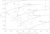 |
Fig. 4 Luminosity estimates (in units of the solar luminosity) plotted against effective-temperature estimates for our binary sample in Table 3 (triangles), together with representative error bars. Also shown are the single-star sample discussed in Sect. 4.4.2 (crosses – some targets have been moved slightly in effective temperature or gravity in order to improve clarity). Evolutionary models (solid lines) of Brott et al. (2011a) are shown for zero initial rotational velocity together with the initial mass (in units of the solar mass). Isochrones (dashed lines) are shown for ages of 5, 10 and 20 Myr. |
Luminosities have been estimated for the binary systems for which a full analysis was undertaken together with those for the equivalent sample of presumed single targets from the VFTS discussed in Sect. 4.2. Interstellar extinctions have been estimated from observed B − V colours provided in Paper I, together with the intrinsic-colour–spectral-type calibration of Wegner (1994) plus RV = 3.5 from Doran et al. (2013). Bolometric corrections were obtained from LMC-metallicity tlusty models (Lanz & Hubeny 2007) for the primary component, and together with an adopted distance modulus of 18 5 for the LMC permitted the systemic luminosity to be estimated.
For one target, VFTS 017, optical photometry was not available and we used the HST photometry of Sabbi et al. (2016) in the F555W band, together with a E(B − V) = 0.31 (average of that found for other B-type stars in VFTS) to estimate a logarithmic luminosity of 4.85 (in units of the solar luminosity). We note that this agrees well with the estimate for VFTS 534, which has similar atmospheric parameters. The estimates are listed in Table 1.
The values for the binary sample should be treated with some caution. For example, a significant secondary contribution of the flux in the V photometric band would lead to an overestimation of the primary’s luminosity. For a 20% secondary flux contribution, this would translate to an overestimate of approximately 0.1 dex. Additionally the presence of a cooler secondary could lead to an overestimation of the reddening leading in turn to an overestimation of the luminosity. However, this effect is likely to be relatively small as any secondary making a significant contribution to the total flux would have a similar colour to the primary. Given the uncertainty in the contribution of the secondary to the total luminosity, a conservative error estimate of ± 0.2 dex has been adopted.
The HR diagram for both the binary and single samples is shown in Fig. 4, together with the same evolutionary tracks and isochrones of Brott et al. (2011a) as shown in Fig. 3. These lead to age estimates similar to those found in Sect. 4.2, with for example, the binaries having a typical age of 10 Myr. One target, VFTS 662, again has an age of more than 20 Myr. The single stars cover a similar range of age estimates. In this case, three targets appear to have age estimates greater than 20 Myr, which would be consistent with the larger sample size.
4.4. Nitrogen abundance
4.4.1. General characteristics
The LMC baseline nitrogen abundance has been estimated from observations of both H ii regions (see, for example, Kurt & Dufour 1998; Garnett 1999) and early-type stars (see, for example, Korn et al. 2002, 2005; Hunter et al. 2007; Trundle et al. 2007). The different studies are in good agreement and imply a value of approximately 6.9 dex, which will be adopted here.
Our nitrogen abundances estimates for the fully analysed binary sample (see Table 3) are in general similar to this baseline LMC abundance. For example, assuming no flux contribution from the secondary, four out of the five targets with specific estimates show an enhancement of less than 0.2 dex. For those targets with upper limits, eleven out of fifteen have enhancements of 0.2 dex or less (with, of course, it being possible that the other four targets also have small enhancements). The results for the targets where no reliable effective temperature could be estimated (see Table 4) are also compatible with relatively modest enhancements. For example, for the five stars where a range in nitrogen abundances could be estimated, three show effectively no enhancements, whilst the other two show enhancements of approximately 0.1–0.3 dex. For both samples, including a contribution from a secondary would increase the actual or possible enhancements but they would still remain relatively modest.
As discussed in Sect. 3.1, our grid of model atmospheres assumed a normal helium and hydrogen abundance ratio. The LMC evolutionary models of Brott et al. (2011a) appropriate to B-type stars indicate that even for a nitrogen enhancement of 1.0 dex (larger than that observed in our sample – see Tables 3 and 4), the change in the helium abundance is typically only 0.03 dex. Hence our assumption of a normal helium abundance is unlikely to be a significant source of error.
Both the Tarantula and FLAMES-I samples were restricted to stars with low projected rotational velocities. We would expect the majority of these stars to also have small equatorial rotational velocities for the following reasons:
-
1.
assuming a random distribution of axes of inclination, theprobability of observing small angles of inclination (and hencesmall sini) is low. For example a sini ≤ 0.25 would only occur in approximately 3% of targets.
-
2.
the identification of binaries will be biased towards systems with large orbital angles of inclination as this will lead to a large range in radial-velocity variations (Dunstall et al. 2015). Surmising that the axes of the orbital and rotational motions are aligned would again favour larger rotational angles of inclination.
The relatively small enhancements in the nitrogen abundances found in the two binary samples would then be consistent with the primaries having evolved as slowly rotating single stars, which have experienced little rotational mixing between the stellar core and envelope. Indeed as discussed by de Mink et al. (2009, 2011), pre-interaction binaries “may provide the most stringent test cases for single stellar models”.
For the Tarantula sample, the range of radial velocity variations for each primary, Δvr, is listed in Table 1. These cover a significant range from approximately 20 to 180 km s-1. Six of the targets have estimates of Δvr of over 100 km s-1and might be expected to be amongst the most tightly bound systems. Inspection of Tables 3 and 4 indicate that (assuming the secondary contributes zero flux) four targets (VFTS 342, 501, 589, 888) have nitrogen enhancements of 0.1 dex or less; two (VFTS 299, 520) have upper limits on the nitrogen abundance of ≤7.3 dex, implying a maximum enhancement of 0.4 dex. Hence for these presumably closely bound systems, there is no evdence of substantial nitrogen abundance enhancements. This provides constraints on the combined effect of the physical processes that would lead to such enhancements. For example, it appears that these closely bound systems binaries have not yet interacted through mass transfer, consistent with the predictions by de Mink et al. (2011, 2014). Additionally it constrains the combined effect of any further mixing processes that may have operated. Specifically, it implies that the effects of rotationally induced mixing have been limited (de Mink et al. 2009; Brott et al. 2011b).
We can compare our nitrogen abundances with those found for the binary VFTS supergiants analysed by McEvoy et al. (2015). Assuming that single star evolutionary models are appropriate, these supergiants will normally have evolved from O-type main sequence stars and hence will not be the descendants of our current sample. McEvoy et al. (2015) found some tentative evidence that low (i.e. near baseline) nitrogen abundances were more prevalent in their B-type primaries. These objects may have evolved from O-type main sequence stars that are analogous to the low nitrogen abundance primaries found in our sample. Additionally McEvoy et al. (2015) identified a small number of binary supergiants with very high nitrogen abundances (~8.0 dex) that showed evidence for being post-interaction systems.
4.4.2. Comparison with single stars
We plot the nitrogen abundance estimates for our binary sample as a function of effective temperature in Fig. 5. The estimates assuming negligible flux contribution from the secondary were adopted; adopting a 20% secondary contribution would increase the estimates by typically 0.1–0.2 dex (see Table 3). Also shown are LMC evolutionary tracks for stars with initial masses of 8, 10 and 12 M⊙ and an initial equatorial velocity of approximately 230 km s-1taken from Brott et al. (2011a). These tracks stretch from the zero age main sequence to when the model has a surface gravity, log g ~ 3.4 dex, consistent with the gravity range of our sample. As discussed in Sect. 4.2, an analysis of an equivalent sample of apparently single stars in the VFTS has been carried out by Dufton et al. (in prep.) using similar methods to those used here. These are also plotted in Fig. 5 and were selected using the same criteria as for the binary sample, i.e. vesini ≤ 80 km s-1and excluding supergiants discussed by McEvoy et al. (2015).
For the binary sample, there are a significant number of stars plotted with Teff = 23 000 K. These correspond to the targets listed in Table 4 and in reality will occupy the effective-temperature range ~20 000–26 000 K. Additionally, many of the abundance estimates are upper limits, implying that Fig. 5 should be interpreted carefully.
Nine targets (5 binaries, 4 “single” stars) appear to have nitrogen abundances that are 0.1–0.3 dex below the adopted baseline abundance; this may simply be due to random uncertainties, estimated in Sect. 3.6 as being of the order of 0.2–0.3 dex. Additionally, Table 3 implies that inclusion of a secondary flux would increase our estimates by 0.1–0.2 dex. Indeed the same effect could be affecting our single-star estimates if there were undiscovered binaries. Hence we do not believe that these stars stars provide any convincing evidence for nitrogen abundances that are truly below our adopted baseline.
Both samples appear to contain significant numbers of stars that have nitrogen abundance estimates close to the assumed baseline abundance of the LMC. Additionally, targets with modest nitrogen enhancements (≤ 0.5 dex) are also observed. As discussed in Sect. 4.4.1, this would be compatible with their evolution as slowly rotating stars with little rotational mixing. One possible difference between the samples is that the single-star sample may contain targets with larger nitrogen abundance enhancements (of up to 1.1 dex). For example, four single stars have estimated abundances that are greater than both the detections and even the highest upper limit found in the binary sample. Such targets have also been found in other presumably single-star samples in the Magellanic Cloud (Hunter et al. 2007, 2008, 2009; Trundle et al. 2007).
The single-star sample consists of 54 targets of which six have nitrogen enhancements of more than 0.6 dex. As discussed in Sect. 4.2, it contains more high mass and hence high effective temperature targets. In particular it has 9 targets that have effective temperatures, Teff> 29 000 K, which is the maximum temperature of the binary sample. Two of these targets show nitrogen enhancements of more than 0.6 dex, leaving 4 (out of 45) targets with significantly enhanced nitrogen in the effective temperature range covered by the binaries. Hence the lack of such objects in the binary sample may at least in part be due the different effective temperature ranges that have been sampled.
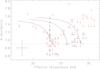 |
Fig. 5 Nitrogen abundance estimates (triangles) and upper limits (arrows) assuming no secondary flux contribution are plotted against effective-temperature estimates for our binary sample (black symbols). The representative error bars are for targets listed in Table 3, with those for targets from Table 4 being larger – see text for details. Also shown are the single-star sample discussed in Sect. 4.4.2 (red symbols – some targets have been moved slightly in effective temperature in order to improve clarity). The dotted line represents a baseline LMC abundance of 6.9 dex. The solid lines are evolutionary models from Brott et al. (2011a) with initial masses of 8, 10 and 12 M⊙ and an initial equatorial rotational velocity of approximately 230 km s-1. |
Statistical comparisons of the binary and single-star samples.
To examine more rigorously the possible differences between binary and single-star samples requires statistical tools. Standard tests for comparing two univariate samples, such as the Kolmogorov-Smirnov and Kuiper tests, are ill-suited to our nitrogen abundance datasets because of the large numbers of upper limits (15/20 and 30/54 for the binary and single-star samples, respectively). However, alternative tools exist for treating data that are randomly censored2. To the extent that detections and limits are intermingled, our abundance results can be approximated as randomly censored datasets (as opposed to being truncated, whereby all detections would lie above a lower-limit cutoff).
We have used the asurv package (v1.2; LaValley et al. 1992), which implements several tests for censored data, to investigate whether the null hypothesis of no differences between the binary and single-star samples can be rejected with appropriate levels of confidence. Results are given in Table 5 for both secondary flux contributions of 0% and 20%. The two-sample (Wilcoxon & logrank) tests are nonparametric comparisons of the distributions, and are moderately insensitive to the details of the censoring (see, e.g., Feigelson & Nelson 1985). None provides any strong evidence for differences between results for the binary and single-star samples, particularly if a modest secondary-flux contribution is accounted for.
The Kaplan-Meier estimator, used to estimate the means of the distributions, is more sensitively dependent on the assumption of truly random censoring. Given this dependence, our interpretation of the results in Table 5 is again that there is no compelling evidence for any overall differences in the single-star and binary nitrogen abundances.
In Sect. 3.6, the He i line at 4009 Å was found to be consistent with secondary flux contribution of between 0 and 20% for the binary sample. Hence we would expect that the use of actual nitrogen abundances (rather than our representative estimates) for the primaries in our binary sample would have led to similar results to those found in Table 5.
As discussed above, the single star sample contains stars with high effective temperatures (>29 000 K) that are not present in the binary sample. We have therefore repeated these tests for those targets within the range, 26 000 ≤ Teff ≤ 29 000 K; the choice of a limited range of effective temperatures should also lead to the two samples having similar ages and masses. For the binary sample, this lead to 14 targets (11 having upper limits for the nitrogen abundance) for a zero secondary flux contribution and 11 targets (and 7 upper limits) for a 20% contribution. For the single star sample, there were 18 targets with 11 upper limits.
The statistical tests are again summarized in Table 5 and in general show no evidence of any difference between the two samples. Indeed the probabilities that the two parent distributions are indistinguishable have increased at least in part due to the smaller sample sizes. Additionally the estimated mean nitrogen abundances of the two samples again show no significant differences.
Therefore we conclude that the statistical tests are consistent with the null hypothesis (that there are no differences between the binary and single-star samples), although in some cases the probabilities listed in Table 5 are relatively small. Indeed Fig. 5 does imply an absence of targets with high nitrogen abundances in the binary sample. As discussed in Sect. 4.4.1, this would be consistent with them having evolved as effectively single stars with low rotational velocities.
The relatively large nitrogen abundances in some of the single stars could then arise from rapidly rotating stars viewed at low angles of incidence. However such viewing angles are unlikely (for example, a value of sini ≤ 0.1 will only occur in 0.5% of targets with randomly aligned rotation axes). This has lead other authors (Hunter et al. 2008; Brott et al. 2011b; Grin et al. 2016) to question whether all the low-vesini single stars with high nitrogen abundances found in other single-star samples can be rapid rotators viewed at low angles of incidence. Indeed other mechanisms (for example, binary mergers, see de Mink et al. 2014) may also be required and this will be considered in detail in Dufton et al. (in prep.).
The binaries discussed here, together with those for the VFTS binary supergiants discussed by McEvoy et al. (2015) are the first significant binary samples to be analysed using model atmosphere techniques. As such they should be considered as pathfinder analyses especially given the difficulty, for example, in allowing for the spectral contributions of unseen secondaries. They should provide a motivation for spectroscopic abundance analysis of larger samples of binary stars, especially given binaries dominate the massive star population (Sana et al. 2012).
“Randomly censored” implies that the probability of the measurement of a given target being an upper limit is independent of the actual value. This may not always be the case here as we would expect to preferentially obtain estimates for targets with large nitrogen abundances. Many of the techniques for characterizing such data were originally developed principally in the field of “survival statistics”, and were first introduced to the astrophysics community by Feigelson & Nelson (1985) and by Schmitt (1985).
Projected rotational velocities are also listed for 16 additional targets that were excluded from Paper II as at that time they were believed to be binaries but have subsequently been designated as “single”. Additionally estimates for 7 targets that are now designated as binaries have been given previously in Paper II.
Acknowledgments
Based on observations at the European Southern Observatory Very Large Telescope in programme 182.D-0222. S.d.M. acknowledges support by a Marie Sklodowska-Curie Action (H2020 MSCA-IF-2014, project BinCosmos, id 661502). R.G. would like to thank the Institute of Physics and the Nuffield Foundation for helping fund this work through their Undergraduate Research Bursary program.
References
- Aerts, C., Molenberghs, G., Kenward, M. G., & Neiner, C. 2014, ApJ, 781, 88 [NASA ADS] [CrossRef] [Google Scholar]
- Brott, I., de Mink, S. E., Cantiello, M., et al. 2011a, A&A, 530, A115 [NASA ADS] [CrossRef] [EDP Sciences] [Google Scholar]
- Brott, I., Evans, C. J., Hunter, I., et al. 2011b, A&A, 530, A116 [NASA ADS] [CrossRef] [EDP Sciences] [Google Scholar]
- Chiosi, C., & Maeder, A. 1986, ARA&A, 24, 329 [NASA ADS] [CrossRef] [Google Scholar]
- de Mink, S. E., Cantiello, M., Langer, N., et al. 2009, A&A, 497, 243 [NASA ADS] [CrossRef] [EDP Sciences] [Google Scholar]
- de Mink, S. E., Langer, N., & Izzard, R. G. 2011, Bull. Soc. Roy. Sci. Liège, 80, 543 [Google Scholar]
- de Mink, S. E., Sana, H., Langer, N., Izzard, R. G., & Schneider, F. R. N. 2014, ApJ, 782, 7 [NASA ADS] [CrossRef] [Google Scholar]
- Donati, J.-F., & Landstreet, J. D. 2009, ARA&A, 47, 333 [NASA ADS] [CrossRef] [MathSciNet] [Google Scholar]
- Doran, E. I., Crowther, P. A., de Koter, A., et al. 2013, A&A, 558, A134 [NASA ADS] [CrossRef] [EDP Sciences] [Google Scholar]
- Dufton, P. L., Ryans, R. S. I., Trundle, C., et al. 2005, A&A, 434, 1125 [NASA ADS] [CrossRef] [EDP Sciences] [Google Scholar]
- Dufton, P. L., Ryans, R. S. I., Simón-Díaz, S., Trundle, C., & Lennon, D. J. 2006, A&A, 451, 603 [NASA ADS] [CrossRef] [EDP Sciences] [Google Scholar]
- Dufton, P. L., Langer, N., Dunstall, P. R., et al. 2013, A&A, 550, A109 [NASA ADS] [CrossRef] [EDP Sciences] [Google Scholar]
- Dunstall, P. R., Brott, I., Dufton, P. L., et al. 2011, A&A, 536, A65 [NASA ADS] [CrossRef] [EDP Sciences] [Google Scholar]
- Dunstall, P. R., Dufton, P. L., Sana, H., et al. 2015, A&A, 580, A93 [NASA ADS] [CrossRef] [EDP Sciences] [Google Scholar]
- Ekström, S., Georgy, C., Eggenberger, P., et al. 2012, A&A, 537, A146 [NASA ADS] [CrossRef] [EDP Sciences] [Google Scholar]
- Evans, C., Hunter, I., Smartt, S., et al. 2008, The Messenger, 131, 25 [NASA ADS] [Google Scholar]
- Evans, C. J., Davies, B., Kudritzki, R.-P., et al. 2011a, A&A, 527, A50 [NASA ADS] [CrossRef] [EDP Sciences] [Google Scholar]
- Evans, C. J., Taylor, W. D., Hénault-Brunet, V., et al. 2011b, A&A, 530, A108 [NASA ADS] [CrossRef] [EDP Sciences] [Google Scholar]
- Evans, C. J., Kennedy, M. B., Dufton, P. L., et al. 2015, A&A, 574, A13 [NASA ADS] [CrossRef] [EDP Sciences] [Google Scholar]
- Feigelson, E. D., & Nelson, P. I. 1985, ApJ, 293, 192 [NASA ADS] [CrossRef] [Google Scholar]
- Fraser, M., Dufton, P. L., Hunter, I., & Ryans, R. S. I. 2010, MNRAS, 404, 1306 [NASA ADS] [Google Scholar]
- Frischknecht, U., Hirschi, R., Meynet, G., et al. 2010, A&A, 522, A39 [NASA ADS] [CrossRef] [EDP Sciences] [Google Scholar]
- Garnett, D. R. 1999, in New Views of the Magellanic Clouds, eds. Y.-H. Chu, N. Suntzeff, J. Hesser, & D. Bohlender, IAU Symp., 190, 266 [Google Scholar]
- Georgy, C., Ekström, S., Eggenberger, P., et al. 2013, A&A, 558, A103 [NASA ADS] [CrossRef] [EDP Sciences] [Google Scholar]
- González, J. F., & Levato, H. 2006, A&A, 448, 283 [NASA ADS] [CrossRef] [EDP Sciences] [Google Scholar]
- Gray, D. F. 2005, The Observation and Analysis of Stellar Photospheres (Cambridge University Press) [Google Scholar]
- Grin, N. J., Ramirez-Agudelo, O. H., de Koter, A., et al. 2017, A&A, 600, A82 [NASA ADS] [CrossRef] [EDP Sciences] [Google Scholar]
- Heger, A., & Langer, N. 2000, ApJ, 544, 1016 [NASA ADS] [CrossRef] [Google Scholar]
- Heger, A., Langer, N., & Woosley, S. E. 2000, ApJ, 528, 368 [NASA ADS] [CrossRef] [Google Scholar]
- Hirschi, R., Meynet, G., & Maeder, A. 2004, A&A, 425, 649 [NASA ADS] [CrossRef] [EDP Sciences] [Google Scholar]
- Howarth, I. D., Dufton, P. L., Dunstall, P. R., et al. 2015, A&A, 582, A73 [NASA ADS] [CrossRef] [EDP Sciences] [Google Scholar]
- Hubeny, I. 1988, Comp. Phys. Commun., 52, 103 [Google Scholar]
- Hubeny, I., & Lanz, T. 1995, ApJ, 439, 875 [Google Scholar]
- Hubeny, I., Heap, S. R., & Lanz, T. 1998, in Properties of Hot Luminous Stars, ed. I. Howarth, ASP Conf. Ser., 131, 108 [NASA ADS] [Google Scholar]
- Hunter, I., Dufton, P. L., Smartt, S. J., et al. 2007, A&A, 466, 277 [NASA ADS] [CrossRef] [EDP Sciences] [Google Scholar]
- Hunter, I., Brott, I., Lennon, D. J., et al. 2008, ApJ, 676, L29 [NASA ADS] [CrossRef] [Google Scholar]
- Hunter, I., Brott, I., Langer, N., et al. 2009, A&A, 496, 841 [NASA ADS] [CrossRef] [EDP Sciences] [Google Scholar]
- Kobulnicky, H. A., Kiminki, D. C., Lundquist, M. J., et al. 2014, ApJS, 213, 34 [NASA ADS] [CrossRef] [Google Scholar]
- Korn, A. J., Keller, S. C., Kaufer, A., et al. 2002, A&A, 385, 143 [NASA ADS] [CrossRef] [EDP Sciences] [MathSciNet] [Google Scholar]
- Korn, A. J., Nieva, M. F., Daflon, S., & Cunha, K. 2005, ApJ, 633, 899 [Google Scholar]
- Kudritzki, R. P., Castro, N., Urbaneja, M. A., et al. 2016, ApJ, 829, 70 [NASA ADS] [CrossRef] [Google Scholar]
- Kurt, C. M., & Dufour, R. J. 1998, in Rev. Mex. Astron. Astrofis. Conf. Ser., 7, eds. R. J. Dufour, & S. Torres-Peimbert, 202 [Google Scholar]
- Langer, N. 2012, ARA&A, 50, 107 [NASA ADS] [CrossRef] [Google Scholar]
- Lanz, T., & Hubeny, I. 2007, ApJS, 169, 83 [CrossRef] [Google Scholar]
- LaValley, M., Isobe, T., & Feigelson, E. 1992, in Astronomical Data Analysis Software and Systems I, eds. D. M. Worrall, C. Biemesderfer, & J. Barnes, ASP Conf. Ser., 25, 245 [Google Scholar]
- Lefever, K., Puls, J., & Aerts, C. 2007, A&A, 463, 1093 [NASA ADS] [CrossRef] [EDP Sciences] [Google Scholar]
- Maeder, A. 1987, A&A, 173, 247 [NASA ADS] [Google Scholar]
- Maeder, A. 2009, Physics, Formation and Evolution of Rotating Stars (Berlin, Heidelberg: Springer) [Google Scholar]
- Mahy, L., Nazé, Y., Rauw, G., et al. 2009, A&A, 502, 937 [NASA ADS] [CrossRef] [EDP Sciences] [Google Scholar]
- Mahy, L., Rauw, G., De Becker, M., Eenens, P., & Flores, C. A. 2013, A&A, 550, A27 [NASA ADS] [CrossRef] [EDP Sciences] [Google Scholar]
- Markova, N., & Puls, J. 2008, A&A, 478, 823 [NASA ADS] [CrossRef] [EDP Sciences] [Google Scholar]
- Mason, B. D., Hartkopf, W. I., Gies, D. R., Henry, T. J., & Helsel, J. W. 2009, AJ, 137, 3358 [NASA ADS] [CrossRef] [EDP Sciences] [Google Scholar]
- McEvoy, C. M., Dufton, P. L., Evans, C. J., et al. 2015, A&A, 575, A70 [NASA ADS] [CrossRef] [EDP Sciences] [Google Scholar]
- Mokiem, M. R., de Koter, A., Vink, J. S., et al. 2007, A&A, 473, 603 [NASA ADS] [CrossRef] [EDP Sciences] [Google Scholar]
- Pasquini, L., Avila, G., Blecha, A., et al. 2002, The Messenger, 110, 1 [NASA ADS] [Google Scholar]
- Pecaut, M. J., & Mamajek, E. E. 2013, ApJS, 208, 9 [NASA ADS] [CrossRef] [Google Scholar]
- Petermann, I., Langer, N., Castro, N., & Fossati, L. 2015, A&A, 584, A54 [NASA ADS] [CrossRef] [EDP Sciences] [Google Scholar]
- Pfuhl, O., Alexander, T., Gillessen, S., et al. 2014, ApJ, 782, 101 [NASA ADS] [CrossRef] [Google Scholar]
- Puls, J., Vink, J. S., & Najarro, F. 2008, A&ARv, 16, 209 [NASA ADS] [CrossRef] [EDP Sciences] [Google Scholar]
- Ramírez-Agudelo, O. H., Simón-Díaz, S., Sana, H., et al. 2013, A&A, 560, A29 [NASA ADS] [CrossRef] [EDP Sciences] [Google Scholar]
- Ryans, R. S. I., Dufton, P. L., Mooney, C. J., et al. 2003, A&A, 401, 1119 [NASA ADS] [CrossRef] [EDP Sciences] [Google Scholar]
- Sabbi, E., Anderson, J., Lennon, D. J., et al. 2013, AJ, 146, 53 [NASA ADS] [CrossRef] [Google Scholar]
- Sabbi, E., Lennon, D. J., Anderson, J., et al. 2016, ApJS, 222, 11 [NASA ADS] [CrossRef] [Google Scholar]
- Sana, H., de Mink, S. E., de Koter, A., et al. 2012, Science, 337, 444 [Google Scholar]
- Sana, H., de Koter, A., de Mink, S. E., et al. 2013, A&A, 550, A107 [NASA ADS] [CrossRef] [EDP Sciences] [Google Scholar]
- Schmitt, J. H. M. M. 1985, ApJ, 293, 178 [Google Scholar]
- Simón-Díaz, S. 2010, A&A, 510, A22 [NASA ADS] [CrossRef] [EDP Sciences] [Google Scholar]
- Simón-Díaz, S., & Herrero, A. 2007, A&A, 468, 1063 [NASA ADS] [CrossRef] [EDP Sciences] [Google Scholar]
- Simón-Díaz, S., & Herrero, A. 2014, A&A, 562, A135 [NASA ADS] [CrossRef] [EDP Sciences] [Google Scholar]
- Simón-Díaz, S., Herrero, A., Esteban, C., & Najarro, F. 2006, A&A, 448, 351 [NASA ADS] [CrossRef] [EDP Sciences] [Google Scholar]
- Simón-Díaz, S., Herrero, A., Uytterhoeven, K., et al. 2010, ApJ, 720, L174 [NASA ADS] [CrossRef] [Google Scholar]
- Simón-Díaz, S., Godart, M., Castro, N., et al. 2017, A&A, 597, A22 [NASA ADS] [CrossRef] [EDP Sciences] [Google Scholar]
- Trundle, C., Dufton, P. L., Hunter, I., et al. 2007, A&A, 471, 625 [NASA ADS] [CrossRef] [EDP Sciences] [Google Scholar]
- Unsöld, A. 1942, Z. Astrophys., 21, 22 [NASA ADS] [Google Scholar]
- Walborn, N. R. 1972, AJ, 77, 312 [NASA ADS] [CrossRef] [Google Scholar]
- Walborn, N. R., Sana, H., Simón-Díaz, S., et al. 2014, A&A, 564, A40 [NASA ADS] [CrossRef] [EDP Sciences] [Google Scholar]
- Wegner, W. 1994, MNRAS, 270, 229 [NASA ADS] [CrossRef] [Google Scholar]
Appendix A: Estimates of projected rotational velocities
Appendix A.1: Data preparation
The data reduction for the individual exposures followed the procedures discussed in Paper I and Dufton et al. (2013,hereinafter Paper II). Because of the radial-velocity variations due to binarity, care had to be taken when combining exposures. We have undertaken simple numerical experiments to estimate the maximum range in radial velocities (Δvr) of individual exposures that can be combined before the estimation of the projected rotational velocity becomes compromised. The spectrum from a main-sequence tlusty model (Hubeny 1988; Hubeny & Lanz 1995; Hubeny et al. 1998; Lanz & Hubeny 2007; Ryans et al. 2003; Dufton et al. 2005, with an effective temperature of 25 000 K, logarithmic gravity of 4.0 dex and microturbulence of 5 km s-1) was convolved with an appropriate instrumental profile. This was then convolved with a projected rotational broadening function (with a given value of vesini) and the resultant spectrum shifted by a radial velocity Δvr before being combined with the unshifted convolved spectrum. This simulates two observations of the primary of the binary system with a velocity difference, Δvr.
The Si iii line at 4552 Å in the combined spectrum was then analysed using the Fourier-Transform methods discussed in Paper II to yield the “observed” vesini. The results of these simulations are summarized in Table A.1 for different choices of Δvr and vesini. As expected the “observed” vesini estimates are reliable for cases where either Δvr is small and/or vesini is large; these cases lie to the right of the dotted line drawn in the table. Note that as in reality we will be combining typically twelve LR02 exposures that all lie within the radial-velocity range, Δvr, this is a very stringent test and in reality the dotted line is likely to lie further to the left (i.e. at lower values of vesini).
Using these simulations, our analysis procedure was as follows. Firstly all LR02 spectra were combined without any wavelengths shifts using the procedures discussed by Dufton et al. (2013) for single stars. The projected rotational velocity, vesini, was then estimated and if it lay to the right of the dotted line, the estimate was accepted. If it lay on or to the left of this line, the spectra were recombined but shifted using the radial-velocity estimates of Dunstall et al. (2015); this procedure was appropriate for the metal line spectra where no nebular emission was present. A further reduction was also undertaken using spectra from only the best LR02 epoch (in terms of signal-to-noise ratio) plus any other epochs with similar radial velocities (i.e. leading to a range of radial velocities, Δvr ≤ 30 km s-1); this was preferable for the He i features which are affected by nebular emission (see Papers I and II for more details).
Simulation of the effects of radial velocity variations on the estimation of the projected rotational velocity from the Si iii line at 4552 Å.
Appendix A.2: Methodology for estimating projected rotational velocities
The procedures for estimating projecting rotational velocities for the B-type binary sample were very similar to those undertaken by Paper II. In summary, a Fourier-Transform (FT) methodology (Simón-Díaz & Herrero 2007) was employed. This has been used to estimate projected rotational velocities in VFTS main-sequence stars (see, Ramírez-Agudelo et al. 2013, and Paper II) and supergiants (McEvoy et al. 2015) and has also been widely used to study the different mechanisms contributing to the broadening of spectral lines in early-type stars (see, for example Dufton et al. 2006; Lefever et al. 2007; Markova & Puls 2008; Simón-Díaz et al. 2010; Fraser et al. 2010; Simón-Díaz & Herrero 2014; Simón-Díaz et al. 2017).
As discussed by Simón-Díaz & Herrero (2007) the FT method should be able to explicitly separate the rotational broadening from other broadening such as natural, instrumental and natural. The approach relies on the convolution theorem (Gray 2005), viz. that the Fourier transform of convolved functions is proportional to the product of their individual Fourier Transforms. It then identifies the first minimum in the Fourier transform for a spectral line, which is assumed to be the first zero in the Fourier transform of the rotational broadening profile with the other broadening mechanisms exhibiting either no minima or only minima at higher frequencies. Further details on the implementation of this methodology can be found in Simón-Díaz & Herrero (2007) and Paper II.
These estimates were supplemented by fitting rotational broadened profiles directly to the observed spectra. As this approach neglects the contribution of the intrinsic line profile and the instrumental profile, it effectively provides an upper limit (see Paper II for a detailed discussion and comparison of the different approaches) and is used here solely as a consistency check.
Two sets of absorption lines were used, which were identical to those adopted in Paper II. For targets with relatively low projected rotational velocities (vesini ≲ 150 km s-1), metal and non-diffuse He i were adopted; for other targets, both non-diffuse and diffuse He i lines were used. Further details and comparison of results estimated from the two sets of lines can be found in Paper II.
In Tables 6 and 7 (only available at the CDS), the estimates from the individual lines are listed for all the non-supergiant targets that are believed to be the primaries of binary systems – these tables have an identical format to those of Tables 3 and 4 of Paper II, where again further details can be found3.
All Tables
Spectral classifications (from Evans et al. 2015), estimated projected rotational velocity (vesini), typical signal-to-noise ratios (S/N) for the LR02 region (which have been rounded to the nearest multiple of five) and observed ranges of radial velocity variations of the primary, Δvr.
Estimates of the atmospheric parameters for the primaries assuming no secondary flux contribution.
Adopted estimates for the projected rotational velocity (vesini), atmospheric parameters, silicon, magnesium and nitrogen abundance estimates.
Nitrogen abundance estimates and projected rotational velocities for targets for which a reliable effective-temperature estimate could not be obtained.
Simulation of the effects of radial velocity variations on the estimation of the projected rotational velocity from the Si iii line at 4552 Å.
All Figures
|
Fig. 1 An example of the estimation of the microturbulent velocity using the relative strengths of three Si iii lines in VFTS 225. Abundances estimates are shown for vt = 1 (triangles), 3 (stars) and 5 (crosses) km s-1, together with linear least square fits. |
| In the text | |
|
Fig. 2 Comparison of observed and theoretical spectra for the region near the N ii line at 3995 Å. VFTS 575 and VFTS 589 are shown to the left and right respectively. The upper and lower panels have a 0% and 20% (with the theoretical spectra being scaled) contribution from the secondary, |
| In the text | |
|
Fig. 3 Gravity estimates plotted against effective-temperature estimates for our binary sample listed in Table 3 (triangles), together with representative error bars. Also shown is the single-star sample discussed in Sect. 4.4.2 (crosses – some targets have been moved slightly in effective temperature or gravity in order to improve clarity). Evolutionary models (solid lines) of Brott et al. (2011a) are shown for zero initial rotational velocity together with the initial mass (in units of the solar mass). Isochrones (dashed lines) are shown for ages of 5, 10 and 20 Myr. |
| In the text | |
|
Fig. 4 Luminosity estimates (in units of the solar luminosity) plotted against effective-temperature estimates for our binary sample in Table 3 (triangles), together with representative error bars. Also shown are the single-star sample discussed in Sect. 4.4.2 (crosses – some targets have been moved slightly in effective temperature or gravity in order to improve clarity). Evolutionary models (solid lines) of Brott et al. (2011a) are shown for zero initial rotational velocity together with the initial mass (in units of the solar mass). Isochrones (dashed lines) are shown for ages of 5, 10 and 20 Myr. |
| In the text | |
|
Fig. 5 Nitrogen abundance estimates (triangles) and upper limits (arrows) assuming no secondary flux contribution are plotted against effective-temperature estimates for our binary sample (black symbols). The representative error bars are for targets listed in Table 3, with those for targets from Table 4 being larger – see text for details. Also shown are the single-star sample discussed in Sect. 4.4.2 (red symbols – some targets have been moved slightly in effective temperature in order to improve clarity). The dotted line represents a baseline LMC abundance of 6.9 dex. The solid lines are evolutionary models from Brott et al. (2011a) with initial masses of 8, 10 and 12 M⊙ and an initial equatorial rotational velocity of approximately 230 km s-1. |
| In the text | |
Current usage metrics show cumulative count of Article Views (full-text article views including HTML views, PDF and ePub downloads, according to the available data) and Abstracts Views on Vision4Press platform.
Data correspond to usage on the plateform after 2015. The current usage metrics is available 48-96 hours after online publication and is updated daily on week days.
Initial download of the metrics may take a while.