| Issue |
A&A
Volume 602, June 2017
|
|
|---|---|---|
| Article Number | A42 | |
| Number of page(s) | 9 | |
| Section | Extragalactic astronomy | |
| DOI | https://doi.org/10.1051/0004-6361/201630331 | |
| Published online | 02 June 2017 | |
Subarcsecond imaging of the water emission in Arp 220⋆,⋆⋆
1 Chalmers University of TechnologyDepartment of Earth and Space Sciences, Onsala Space Observatory, 43992, Onsala, Sweden
e-mail: This email address is being protected from spambots. You need JavaScript enabled to view it.
2 European Southern Observatory (ESO), Alonso de Córdova 3107, Vitacura, Casilla 19001, 763 0355 Santiago, Chile
3 Joint ALMA Observatory, Alonso de Córdova 3107, Vitacura, Casilla 19001, 763 0355 Santiago, Chile
4 Grupo de Astrofísica Molecular, Instituto de CC. de Materiales de Madrid (ICMM-CSIC), Sor Juana Inés de la Cruz 3, Cantoblanco, 28049 Madrid, Spain
5 Institute of Astronomy and Astrophysics, Academia Sinica, PO Box 23-141, 10617 Taipei, Taiwan
6 Max-Planck Institute for Astronomy, Königstuhl 17, 69117 Heidelberg, Germany
7 European Southern Observatory (ESO), Karl-Schwarzschild-Str. 2, 85748 Garching bei München, Germany
8 Institut de Radioastronomie Millimétrique (IRAM), 300 rue de la Piscine, Domaine Universitaire, 38406 Saint-Martin-d’Hères, France
9 Laboratoire AIM, CEA/IRFU/Service d’Astrophysique, Bât. 709, 91191 Gif-sur-Yvette, France
10 National Radio Astronomy Observatory (NRAO), PO Box O, 1003 Lopezville Road, Socorro, NM 87801, USA
11 New Mexico Institute of Mining and Technology, Socorro, NM 87801, USA
12 Observatorio Astronómico Nacional (OAN, IGN), Apdo 112, 28803 Alcalá de Henares, Spain
13 Observatorio de Madrid, OAN-IGN, Alfonso XII, 3, 28014 Madrid, Spain
Received: 22 December 2016
Accepted: 6 March 2017
Abstract
Aims. Extragalactic observations of water emission can provide valuable insight into the excitation of the interstellar medium. In particular they allow us to investigate the excitation mechanisms in obscured nuclei, that is, whether an active galactic nucleus or a starburst dominates.
Methods. We use subarcsecond resolution observations to tackle the nature of the water emission in Arp 220. ALMA Band 5 science verification observations of the 183 GHz H2O 313 − 220 line, in conjunction with new ALMA Band 7 H2O 515 − 422 data at 325 GHz, and supplementary 22 GHz H2O 616 − 523 VLA observations, are used to better constrain the parameter space in the excitation modeling of the water lines.
Results. We detect 183 GHz H2O and 325 GHz water emission toward the two compact nuclei at the center of Arp 220, being brighter in Arp 220 West. The emission at these two frequencies is compared to previous single-dish data and does not show evidence of variability. The 183 and 325 GHz lines show similar spectra and kinematics, but the 22 GHz profile is significantly different in both nuclei due to a blend with an NH3 absorption line.
Conclusions. Our findings suggest that the most likely scenario to cause the observed water emission in Arp 220 is a large number of independent masers originating from numerous star-forming regions.
Key words: galaxies: individual: Arp 220 / galaxies: ISM / galaxies: starburst / ISM: molecules
Based on observations carried in ALMA programs ADS/JAO.ALMA#2011.0.00018.SV and ADS/JAO.ALMA#2012.1.00453.S, with the IRAM 30 m telescope under project numbers 189-12 and 186-13.
We dedicate this work to the memory of Fred Lo.
© ESO, 2017
1. Introduction
At a luminosity distance of 78 Mpc (1′′ = 378 pc), Arp 220 makes for one of the most interesting objects of study in the nearby Universe. It is a suitable target to examine a large number of different tracers of the interstellar medium (ISM), sampling different physical conditions on a large range of spatial scales. Its high infrared luminosity (LIR = 1.4 × 10¹²L⊙, Soifer et al. 1987) makes Arp 220 a good local proxy for high-redshift (ultra-)luminous infrared galaxies ((U)LIRGs). As a result, we now know that Arp 220 is the result of a merger (Arp 1966; Nilson 1973; Sakamoto et al. 1999) – the two remnant nuclei, Arp 220 East and Arp 220 West, are separated by only ~380 pc at the center of Arp 220 (e.g., Downes & Eckart 2007; Aalto et al. 2009; Sakamoto et al. 2009; Martín et al. 2011). They are each embedded in their own rotating gas disks in the foreground of a kpc-scale molecular gas disk (e.g., Scoville et al. 1997; Sakamoto et al. 1999; König et al. 2012). The different origins of the two nuclei manifest themselves as a misalignment in the rotation axes of the gaseous disks. Whether AGN or the powerful starburst associated with the central activity, or a mixture of the two, facilitates the bright appearance of this prototypical ULIRG at many wavelengths is still under debate (e.g., Smith et al. 1998; Lonsdale et al. 2006; Downes & Eckart 2007; Sakamoto et al. 2008).
The physical conditions in Arp 220 have been probed using a number of tracers at radio, mm and submm wavelengths (e.g., Scoville et al. 1997; Sakamoto et al. 1999, 2008, 2009; Aalto et al. 2007; Aalto et al. 2009, 2015; Downes & Eckart 2007; Martín et al. 2011, 2016; González-Alfonso et al. 2012; König et al. 2012; Wilson et al. 2014; Aladro et al. 2015; Rangwala et al. 2015; Scoville et al. 2015; Tunnard et al. 2015; Martín et al. 2016; Varenius et al. 2016). Among others, the water lines in the radio and mm wavelength regimes have been targeted (e.g., Cernicharo et al. 2006b; Galametz et al. 2016; Zschaechner et al. 2016). Water emission is an excellent tracer of physical conditions, such as temperature and density of the molecular gas, in the highly obscured innermost parts of external galaxies. The water lines at 22, 183, 321 and 325 GHz rest frequency have been observed as masers in various galactic sources (e.g., in star-forming regions and circumstellar envelopes around evolved stars, Cernicharo et al. 1990, 1994, 1996, 1999; Gonzalez-Alfonso et al. 1995, 1998; González-Alfonso & Cernicharo 1999; De Buizer et al. 2005; Lefloch et al. 2011; Bartkiewicz et al. 2012; Richards et al. 2014, and references therein). In extragalactic sources, the 22 GHz line is most commonly used to search for maser emission – more than 150 sources have been found to emit water maser emission, mostly in galaxies with active galactic nuclei (AGN, e.g., Lo 2005; Pesce et al. 2016). The 183 GHz line has been detected toward NGC 3079 (Humphreys et al. 2005), Arp 220 (Cernicharo et al. 2006b; Galametz et al. 2016), and most recently toward NGC 4945 (Humphreys et al. 2016). In both NGC 3079 and NGC 4945, the 183 GHz maser emission is associated with the AGN. This seems also true for the water maser emission at 321 GHz that was recently reported toward Circinus and NGC 4945 (Hagiwara et al. 2013, 2016; Pesce et al. 2016). All these are classified as megamasers, that is, the isotropic luminosity is higher by a factor of more than 106 times than what is found for typical emission of Galactic water masers (at 22 GHz: ~10-4L⊙, e.g., Lo 2005). Recently, the 22 GHz H2O 615 − 523 has been tentatively detected in both nuclei in Arp 220 (Zschaechner et al. 2016). At 183 GHz, single-dish observations yielded convincing evidence for the presence of emission of the H2O 313 − 220 line in emission (Cernicharo et al. 2006b; Galametz et al. 2016).
Cernicharo et al. (2006b) presented a first analysis of the 183 GHz water emission in Arp 220 and showed that a combination of the three major water lines at 22, 183, and 325 GHz is necessary to properly model the excitation in the galaxy center. In this paper, we combine subarcsecond-scale ALMA observations of H2O 22 and 325 GHz with the 183 GHz line resolved for the first time with the newly installed ALMA Band 5 receivers (Belitsky et al. 2009; Billade et al. 2010) to refine the modeling of the excitation conditions in Arp 220.
In Sect. 2 the observations, data reduction and analysis are described, in Sect. 3 we present the results, and in Sect. 4 we discuss their implications.
2. Observations
Water line properties.
2.1. ALMA
2.1.1. Band 5
ALMA observations of the H2O 313 − 220 line at 183.310 GHz rest frequency in Arp 220 were obtained on 2016 July 16th, as part of the Band 5 science verification observations. The dual polarization Band 5 receivers, designed and developed by the Group for Advanced Receiver Development at Chalmers University and Onsala Space Obervatory (GARD, Sweden) and the STFC Rutherford Appleton Laboratory (UK), cover the frequency range between 163 and 211 GHz. The receivers provide separated sidebands and an instantaneous bandwidth coverage of 8 GHz (Belitsky et al. 2009; Billade et al. 2010, 2012). The array was composed of 12 antennas equipped with Band 5 receivers, in a configuration with baselines ranging from 30 m to 480 m. The weather conditions were excellent – approximately 0.3 mm precipitable water vapor. One spectral window, with a bandwidth of 1.875 GHz and spectral resolution of 976.562 kHz, was centered on the water line. Additional spectral windows were placed on the HNC 2−1, CS 4−3, and CH3OH 431 − 330 transitions, with bandwidths of 1.875 GHz and 0.9375 GHz, at spectral resolutions of 976.562 kHz and 488.281 kHz, respectively. For analysis purposes, the resolution was averaged to 20 km s-1 channels. The bandpass response of the antennas was calibrated from observations of the bright quasar J1924-2914, with J1516+1932 being used for primary gain calibration, and J1550+0527 for flux calibration. The continuum emission is strong enough for self-calibration of the data. However, it was difficult to determine line-free channels to derive the continuum contribution, especially for Arp 220 West. A model of the source was constructed after a shallow clean, using line-free channels in spectral windows 2 and 3 (upper sideband). Then, gain phase solutions were determined for each integration and applied to all spectral windows, including the lower sideband. The calibrated visibilities were deconvolved using the “tclean” task in CASA 4.7.01 (McMullin et al. 2007) resulting in a beam size of 0.79′′ × 0.71′′ (~0.30 kpc × 0.27 kpc), and individual data cubes were created for each spectral window. The resulting sensitivities are shown in Table 1. After calibration and imaging within CASA, the visibilities were converted into FITS format and imported in the GILDAS/MAPPING2 for further analysis.
2.1.2. Band 7
The Band 7 ALMA data covering the H2O 515 − 422 line at 325.153 GHz rest frequency were obtained on 2014 June 16 and July 17, as part of a full spectral line survey of ALMA Bands 6 and 7 (Martín et al., in prep.; Project 2012.1.00453.S). The array was composed of 39 antennas. The data were self-calibrated and smoothed to channel widths of 10 MHz. A more detailed description of the calibration of the data will be presented in Martín et al. (in prep.). For analysis purposes, the channels were further binned to widths of 20 km s-1. The calibrated visibilities were imaged to match the spatial and spectral resolution of the Band 5 data.
2.1.3. Contribution of line blending
Since the mm spectrum of Arp 220 contains numerous spectral lines (see e.g., Martín et al. 2011), we carefully investigate the potential contamination by other species. Both the 183 and 325 GHz water lines are affected by blending with other molecular transitions. To correctly estimate the water line intensities, taking into account this contribution from other species, we used the synthetic spectrum model fit to Band 6 and 7 observations (Martín et al., in prep.). The model fit was performed assuming LTE conditions and includes the contribution from more than 30 species, isotopologs and vibrationally excited states. At 183 GHz we use the synthetic spectrum and extrapolate the model fit to Band 5. Figure 1 shows that the extrapolation to Band 5 appears to properly fit the emission outside the water line. The main contribution to the observed profile around this water line is the emission of both C2H5CN and HC3N v7 = 2 at 183.1 GHz and the c-C3H2 at 183.6 GHz. The main contaminants to the 325 GHz H2O line are CH2NH emission at 325.3 GHz, and to a lesser extent, CH3CCH emission at 324.6 GHz.
 |
Fig. 1 Water emission from Arp 220 West (black) and Arp 220 East (red) at 22 (left), 183 (center) and 325 GHz (right). The spectra were extracted from data convolved with the same beam of 0.79′′ × 0.71′′. An artificial offset in intensity was introduced to better show the spectra for each nucleus separately. The dotted lines show the zero-intensity levels. The 22 GHz spectrum has been corrected for contamination by the NH3 (3,1) absorption line. The dark and light blue curves in the 183 and 325 GHz spectra represent the synthetic spectrum used to evaluate the contamination of the water line by other emission lines (Martín et al., in prep.). |
 |
Fig. 2 Maps of the integrated intensity distributions (left) and the velocity fields (right) of the 183 and 325 GHz water lines. Integrated intensity maps: phase center is located at Arp 220 West (α = 15:34:57.220, δ = +23:30:11.60). The contours start at 5σ and are spaced in steps of 10σ (1σ(183 GHz) = 3.9 mJy km s-1, 1σ(325 GHz) = 5.4 mJy km s-1). Velocity fields: color scale is identical for both lines (5200 km s-1–5600 km s-1) and the velocity contours start at 5280 km s-1 and are spaced in steps of 30 km s-1. North is up, east to the left. The beam (0.79′′ × 0.71′′) is indicated in the bottom right corner of each image. The bar in the lower left corner represents a spatial scale of 200 pc. |
All flux values for the interferometrically observed water lines stated from this point on refer to the spectra corrected for their contaminants, and should thus only contain contributions by the corresponding water lines.
2.2. IRAM 30 m
IRAM 30 m observations of the H2O 313 − 220 and H2O 515– 422O lines (νrest = 183.310 GHz, and 325.153 GHz respectively) toward the center of Arp 220 were performed in December 2012 (project: 189-12, PI: J. Cernicharo) and April/May 2014 (project: 186-13; Krips et al., in prep.). The beam sizes of the IRAM 30 m telescope at these frequencies are 14′′ and 8′′. We used EMIR in conjunction with the FTS backend at a spectral resolution of 0.2 MHz over a bandwidth of 4 GHz (~4000 km s-1 and ~6750 km s-1, respectively). Regular pointing and focus measurements on bright nearby quasars and a line source to verify the absolute flux calibration were conducted. Typical system temperatures were Tsys ≃ 300–1400 K at 2 mm and Tsys ≃ 300–1200 K at 0.8 mm – the high Tsys values are due to the fact that the edges of the observed frequency bands are close to the atmospheric water absorption lines around 183 GHz and 325 GHz. We converted  scales using
  with the following efficiencies taken from the IRAM 30 m webpage: Feff = 0.93 and Beff = 0.74 at 180 GHz and Feff = 0.81 and Beff = 0.35 at 320 GHz sky frequency.
2.3. 22 GHz VLA data
The VLA H2O 616 − 523 line at 22.235 GHz rest frequency is blended with the NH3 (3,1) absorption line, with a major effect toward Arp 220 West (see Fig.3 in Zschaechner et al. 2016). In order to retrieve the intrinsic profiles of the 22 GHz water line, we simultaneously fit the NH3 lines within the VLA spectrum closest to the water line: NH3 (3,1) (rest frequency: 22.235 GHz) and NH3 (4,2) (rest frequency: 21.703 GHz). We assume a simple Gaussian line profile, with the same centroid velocity and linewidth for both lines, and a relative intensity scaling between NH3 (4,2) and NH3 (3,1). We find v0 = –94.5 ± 5.5 km s-1, FWHM = 287 ± 13 km s-1, and a line ratio NH3 (4,2)-to-NH3 (3,1) of 1.14 ± 0.08. A comparison of the spectra before and after the fit is shown in Fig. A.1. For Arp 220 East, the NH3 absorption is weak relative to the H2O line. Thus we keep the original water spectrum without trying to correct for NH3 absorption. To be able to compare these data to the water lines at 183 and 325 GHz, the spatial and spectral resolution were degraded to the coarser resolution of the Band 5 data (~20 km s-1, 0.79′′ × 0.71′′).
3. Results
3.1. Water
183 GHz. The emission from the H2O 313 − 220 line is detected in both nuclei (Figs. 1, 2). The brightest flux is found in Arp 220 West (integrated intensity: ~47.8 Jy km s-1). Arp 220 East is approximately three times less luminous (~13.7 Jy km s-1). The velocity field shows a much steeper gradient in Arp 220 East than in Arp 220 West (Fig. 2). 325 GHz. For the first time we detect the 325 GHz H2O 515 − 422 line in an extragalactic environment. Both, single-dish (IRAM 30 m) and interferometric observations (ALMA), led to detections of this water transition (Figs. 1–3, see also Table 1). Similar to the 183 GHz line, 325 GHz emission is found in both nuclei, with Arp 220 West being the brightest. Integrated fluxes amount to ~25.3 Jy km s-1 and 9.1 Jy km s-1 in Arp 220 West and East, respectively. The velocity field (Fig. 2) shows a similar behavior between Arp 220 East and Arp 220 West as at 183 GHz. 22 GHz. The correction of the H2O 616 − 523 emission line for the NH3 (3,1) absorption leaves us with a picture opposite to what we find for the 183 and 325 GHz water lines: the 22 GHz emission is brightest in Arp 220 East (Fig. 1, integrated intensity: ~0.34 Jy km s-1). The emission in Arp 220 West, however, is relatively faint (~0.17 Jy km s-1), which is surprising. One caveat the NH3 (3,1) leaves us with, is that the two emission peaks in Arp 220 East could actually be not two separate peaks but one broad line with the NH3 absorption on top of the water line. If this is the case, then the 22 GHz water line in Arp 220 East is even brighter than what we take into account here. This could also mean that the majority of the 22 GHz line in Arp 220 West is absorbed so that we are missing this velocity component, which would also explain the apparent misalignment of the velocities between the eastern and western nuclei visible in Fig. 1. A contribution of the 13CH3OH line as mentioned in Zschaechner et al. (2016) is very unlikely; this line has not been detected in any of the broad frequency spectral scans conducted in Arp 220 so far (e.g., Martín et al. 2011; Aladro et al. 2015).
3.2. Other identified lines in Band 5
Other detected lines included in the Band 5 tuning are HNC 2−1, CH3OH 4−3, and CS 4−3 (see Fig. B.1). These lines have been previously observed with SEPIA at APEX by Galametz et al. (2016). Furthermore, fainter lines identified within the respective frequency ranges are vibrationally excited HC3N (several lines close to H2O 313 − 220) and CH3CN 10−9 (see also Table B.1), as well as potentially H13CCCN, C34S 4−3 and 13CH3CN. They have been identified using the synthetic spectrum extrapolated from Bands 6 and 7 (Martín et al., in prep.) to Band 5 (see Sect. 2). Most of these lines are fainter in Arp 220 East than in Arp 220 West. They all have been previously detected at 1 and/or 3 mm by Martín et al. (2011) and Aladro et al. (2015), for example.
4. Discussion
In 2006, Cernicharo et al. observed the H2O 313 − 220 line at 183 GHz rest frequency for the first time in Arp 220. Its isotropic luminosity placed it firmly in the range of megamasers. This detection was later confirmed by Galametz et al. (2016). The absence of time variations in the line in-between the two observing periods and the similar line profile to H218O (Martín et al. 2011) led to speculations about the origin of the water emission: both analyses favor thermal processes and/or a large number of star-forming cores as the cause of the observed water signature, rather than an AGN maser origin. However, at the time Cernicharo et al. (2006b) performed the modeling only information about the spatially unresolved 183 GHz line was available. The authors concluded that only a combination of the three major water lines at 22, 183, and 325 GHz would provide a clear picture of the excitation conditions in the molecular gas emitting water emission in Arp 220. Their excitation analysis was further limited by the lack of spatial resolution. Hence, this work, where we make use of subarcsecond-scale observations of all three lines, does represent a major step forward in finding the true powering source of the bright water emission in Arp 220.
4.1. Time variability
We compare the line contamination uncorrected ALMA Band 5 data with previous single-dish spectra from the IRAM 30 m and APEX (see Table 1). A degradation of the convolving beam allows us to compare to what has been found by Cernicharo et al. (2006b) and Galametz et al. (2016, Fig. 3. The flux recovered from the degraded ALMA data (35′′ aperture) is ~56.0 Jy km s-1. This is 10% larger than the flux found by Galametz et al. (2016), which matches their measurement uncertainties. Line shapes and widths (FWHM) are in agreement as well: 318 km s-1 versus 310 km s-1 from Cernicharo et al. (2006b), and 332 ± 31 km s-1 from Galametz et al. (2016).
We also degraded the ALMA 325 GHz data to the same beam size as the IRAM 30 m observations (8′′, Fig. 3). The integrated intensity determined from the ALMA data (~45.4 Jy km s-1) is slightly higher than what we find for the IRAM 30 m observations (~39.8 Jy km s-1 in December 2012, and ~42.3 Jy km s-1 in April/May 2014). However, the signal-to-noise ratio in the IRAM data was relatively low compared to the higher sensitivity ALMA data set, which also necessitated a comparatively heavy spectral binning, making the determination of the FWHM line width difficult. The extracted FWHMs are ~440 km s-1 for ALMA and ~445 km s-1 for the IRAM 30 m spectra (Fig. 3).
The shortest baselines in the ALMA observations correspond to spatial frequencies of ~11′′ (Band 5) and ~14′′ (Band 7). Thus the interferometer should recover all structures ≤5′′ that are larger than the size of the two nuclei (e.g., Downes & Eckart 2007; Aalto et al. 2009; Sakamoto et al. 2009; Martín et al. 2011). The consistency between the contamination-uncorrected ALMA Band 5 and single-dish spectra (intensity, line shape, see Fig. 3) suggests that the water line did not vary in time in between observations. The lack of variability in the lines gives us further confidence that the line ratios used in the LVG modeling below, are robust despite being observed at different times. Typical timescales on which those variations are expected for extragalactic water megamaser emission can range from minutes to days to weeks to months to years (e.g., Greenhill et al. 1997; Raluy et al. 1998; Braatz et al. 2003; Lo 2005, and references therein).
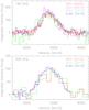 |
Fig. 3 Comparison of the intensities and line shapes between previous single-dish observations (IRAM 30 m, APEX) and spatially smoothed ALMA observations at 183 and 325 GHz. The spectra are in good agreement within the errors imposed by the differences in the sensitivity of the used instruments. |
4.2. Line morphology
4.2.1. Ratios
Peak brightness temperatures and their ratios.
A comparison of the integrated intensity values given in Sect. 3.1 shows that the integrated intensity 183-to-325 GHz ratios for the two nuclei, IWest (183 GHz)/IWest (325 GHz) and IEast (183 GHz)/IEast (325 GHz), are 1.9 and 1.5, respectively. The intensity ratios between the nuclei at each of the two frequencies differ as well: I183 (West)/I183 (East) ~3.5 and I325 (West)/I325 (East) ~2.8.
The observed peak brightness temperatures at 22, 183 and 325 GHz are comparable: 6.6 K at 22 GHz (in Arp 220 East, see also Table 2), 11.1 K at 183 GHz (in Arp 220 West), 2.1 K at 325 GHz (in Arp 220 West). These temperatures are much lower than what is typically expected for maser emission (~109−10 K or more; Slysh 2003; Cernicharo et al. 2006a; Cesaroni 2008; Gray 2012, and references therein). Thus, despite the high isotropic luminosity, and together with the lack of variability at 183 and 325 GHz it seems unlikely that the water emission in Arp 220 could have a maser origin if coming from one large cloud (e.g., of the size of the beam) surrounding the nuclei. A thermal origin was suggested as an alternative by Martín et al. (2011) and Galametz et al. (2016). However, thermal emission from the three lines seems unlikely as the 22 GHz line arises from an energy level Eupper at 609 K (see Table 1) which will require very specific physical conditions to have pure thermal emission. Moreover, the observed line intensity ratios are not compatible with pure thermal emission. Hence, it is very likely possible that the emission region is much smaller than the beam size we reach in this work, for example, a large number of smaller clumps emitting in the water lines. Consequently, the corresponding brightness temperatures would rise considerably above the values measured here. High angular resolution observations with the most extended configurations of ALMA are needed to determine the true projected surface area of the H2O emission.
4.2.2. Line shapes
Compared to extragalactic maser emission, for example in Circinus (e.g., Hagiwara et al. 2013, 2016; Pesce et al. 2016), the line shapes of the 183 GHz and 325 GHz water lines in Arp 220 are rather unspectacular. The complex velocity structure with multiple narrow features commonly associated with megamaser emission is not apparent in Arp 220. The contamination-free spectra show broad emission lines (FWHM ~ 318 km s-1) that are uniform in their structure (Fig. 4). In Arp 220 East, the emission lines have a boxy, double-peaked, non-Gaussian appearance. In Arp 220 West the spectra are single-peaked symmetric and Gaussian-like. This is also corroborated in the velocity fields at both frequencies (Fig. 2). Extragalactic sources exhibiting maser lines of complex velocity structure are typically those where the maser is associated with the accretion disk or torus close to an AGN. These so-called disk-masers are mostly found in Seyfert 2 and LINER galaxies (low ionization emission region, e.g., Kartje et al. 1999; Kuo et al. 2011, 2015). In other galaxies, megamaser emission is caused by the interaction between the AGN jet and molecular clouds in the surrounding interstellar medium (jet-masers, e.g., Mrk 348; Peck et al. 2003; Castangia et al. 2016). The maser lines in these sources are typically as featureless as what we find in Arp 220. However, a comparison of the velocity distributions in the water emission in Arp 220 to, for example, the CO 1−0 velocity field (e.g., Scoville et al. 2017), shows a similar rotation pattern. Thus, it seems unlikely that the maser emission is due to an interaction between an AGN jet and molecular clouds in its vicinity. The signature of this process would introduce a disturbance in the velocity field that would be apparently different from the rotation pattern observed at the spatial and spectral resolutions in the data. A complementary scenario previously suggested to explain the maser emission in Arp 220 is that it originates from a large number of star-forming cores, comparable to what has been found in Sgr B2 (Cernicharo et al. 2006b; Galametz et al. 2016). Indeed, high-resolution VLBI observations have discovered almost fifty point sources in the central 0.5 kpc that have been identified as radio supernovae (RSNe) and supernova remnants (SNRs, Smith et al. 1998; Lonsdale et al. 2006; Parra et al. 2007; Batejat et al. 2011), pointing toward very active star formation. In fact, with a star formation rate of few 100 M⊙ yr-1 (e.g., Anantharamaiah et al. 2000; Thrall 2008; Varenius et al. 2016), it is certainly possible that the brightness of water lines observed in Arp 220 is entirely due to the emission from a large number of star-forming regions.
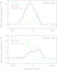 |
Fig. 4 Comparison of the line shapes and peak temperatures of the contamination-corrected water spectra at 22 (in green), 183 (blue), and 325 GHz (red) in Arp 220 West (top) and East (bottom). |
4.3. Excitation
In the following discussion, we assume that the observed 22 GHz emission is real and that its observed intensity has an uncertainty of 50% due to the strong contamination by NH3. The three lines observed in this paper arise from upper energy levels at 205 K (183 GHz), 470 K (325 GHz), and 609 K (22 GHz; the given levels correspond to the ortho species which is 34 K above the para one) and have Einstein coefficients of 3.62 × 10⁻⁶ s-1, 1.15 × 10⁻⁵ s-1 and 1.98 × 10⁻⁹ s-1 respectively. Hence, excitation conditions could be very different for the three lines and the observed emission could trace different regions of the clouds. A comparison of the expected brightness temperatures of the three lines at 22, 183, and 325 GHz in Arp 220 was previously made by Cernicharo et al. (2006b). Here we repeat these calculations using new collisional rates of Daniel et al. (2011), including dust emission excitation effects on the population of the rotational levels of H2O. In all cases, we assumed that the main collider is ortho H2. Dust emission will affect the range of volume and column densities under which these lines will have a significant emission in Arp 220. For the far-IR lines of water vapor observed in this source, González-Alfonso et al. (2004, 2012) concluded that all the lines were formed around the optically thick continuum sources in the two nuclei of Arp 220. The dust opacity is so large that these lines appear in absorption as they are subthermally excited. However, the 22, 183, and 325 GHz lines observed here appear in emission and collisional excitation does play an important role in the emerging intensity. Moreover, unlike the far-IR lines that cannot give information about regions of high dust opacity, the three submillimeter, millimeter, and radio lines considered here could transport some information from these regions.
We have modeled the water emission at 22, 183, and 325 GHz in Arp 220 using the MADEX code (Cernicharo 2012). The model includes a central source of dust emission to assess the effect of the dust on the expected intensity of the lines. Figure 5 shows the predicted intensities for a large range of H2 densities, gas temperatures (50 to 300 K), and column densities N(H2O)/Δv (4 × 10¹⁶ to 4 × 1018 cm-3 (km s-1)-1). As for other water maser models, such as, for example, Neufeld & Melnick (1991), we assume an ortho-to-para ratio of 3:1. Solid lines represent the expected intensities without continuum emission while dashed lines show the results when infrared pumping from dust is taken into account. The central source has a size of 5 pc and the layer of water vapor was placed at a distance of 1.5 pc from the outer radius of the continuum source. As expected, the effect of infrared pumping is a reduction of the maser effect (in particular for the 22 GHz line) and a shift of the intensity maximum toward higher densities. For low gas densities and temperatures, the presence of infrared pumping significantly increases the emission of the three water lines. The predicted brightness temperatures, in absence of dust, agree very well with those of Cernicharo et al. (2006b). As the density and gas temperature increase, masing effects do appear in a similar way than what has been found in their work. Placing the layer of water vapor at larger distances from the continuum dust emission source reduces the infrared pumping considerably.
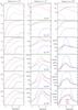 |
Fig. 5 LVG models covering a wide range of physical conditions for three different column densities. For six different kinetic temperatures (TK), the gas temperature variation over a range of H2 densities is shown. The blue, black, and red colors represent the results for the 22, 183, and 325 GHz lines, respectively. Solid lines represent the expected intensities without continuum emission while dashed lines show the results when infrared pumping from dust is taken into account. |
To pinpoint the range of parameters describing the physical conditions in the emission regions of the water lines Arp 220, we start from the most simple assumption: the water emission at 22, 183, and 325 GHz arises from one single large cloud. If a continuum source is not considered, the observed intensities of the 183 GHz and 325 GHz lines alone could be reproduced simultaneously within a parameter space of n(H2) = 104–105 cm-3, TK = 100 K, and N(H2O)/Δv = 4 × 1017 cm-3 (km s-1)-1. If dust emission is taken into account, no solution can be found for the 183 and 325 GHz lines. On top of that, both these models fail to reproduce the 22 GHz line. It is thus not possible to converge on a solution for this most simple scenario.
Therefore, our next approach is to model the water emission as originating from several smaller clouds. To estimate the impact of the number and size of the clouds, we introduce a dilution factor d. The dilution factor is a measure of the area occupied by a structure of radius r inside the region covered by the beam: (r/rbeam)2 (for one source). For N sources, the dilution factor will be  . A dilution factor of 1 means that the solid angle of the source is equal to the solid angle of the beam. If d is 0.1, 10% of the beam area is filled by the source(s). A d of 0.001 means that the emission is coming from a small fraction of the beam. The dilution factor also has an influence on the true brightness temperature – TB/d.
Assuming that the water emission originates from a number of smaller clouds does indeed result in a common solution for all three lines – for large dilution factors d at high column densities (N(H2O)/Δv = 4 × 1018 cm-3 (km s-1)-1) and high temperatures (TK = 200–300 K). If no continuum source is present, the dilution factors we have to apply are 0.005 for TK = 200 K and 0.0025 for TK = 300 K. The density for which this solution is found is rather low, around 8 × 104 cm-3. If the continuum source is present, the dilution factor has to be 0.001 for TK = 200 K and 0.0007 for TK = 300 K. In this case, the density is ≃106 cm-3. In both cases the three lines are masing. The large dilution factors we derive imply a large number of small sources inside the beam. As a reference, the extremes of the estimated dilution factors of 0.0007 and 0.005 would be equivalent to a single source of 0.018′′ (7 pc) and 0.05′′ (18 pc), or a large number of smaller sources. This is also what has been previously suggested by Cernicharo et al. (2006b) and Galametz et al. (2016).
The above estimations assume the same dilution factor applied for the three lines, which is of course very unlikely if we consider what is known for the emission of these lines in galactic sources (see Sect. 4.2). This, however, it is the best we can do with the limited information we have so far on the spatial extent of the emission. Moreover, the lack of information about the position of the sources relative to the continuum dust emission introduces large uncertainties in the estimated densities and temperatures. In addition, the solution found fitting all three lines has to be taken with caution in view of the uncertainties in the emission of the 22 GHz line.
We conclude that the most plausible origin of the observed emission is that a large number of small dense and warm molecular clouds, strongly diluted in our 0.7′′ angular resolution synthetic beam, are present around the nuclei of Arp 220. A solution involving moderate densities of 104−5 cm-3 and TK = 100 K is also possible but fails to reproduce the 22 GHz line. For the same column density of water, the 183 and 325 GHz lines could be also fitted with higher densities if we assume a dilution factor for the emitting clouds. Due to the peculiar physical conditions needed to pump the 183 and 325 GHz lines (see Table 1) – they originate from spatial sizes much larger than those corresponding to the 22 GHz maser emission (e.g., Cernicharo et al. 1990, 1994) – higher spatial resolution observations with ALMA of these lines could provide strong constraints on the physical conditions of the molecular clouds of Arp 220: If one were to assume that the ensemble of clouds from which the emission at 183 and 325 GHz originates in Arp 220 occupies similar size scales to, for example, the emission region in Sgr B2 (about 25 pc, e.g., Scoville et al. 1975), then the Arp 220 emission region would be at least a factor of 10 smaller than the beam size in our data (~0.06′′ at the Arp 220 distance). Distinct regions exhibiting maser emission in Sgr B2 have sizes of approximately 0.7 pc (e.g., de Vicente et al. 1997), which at the distance of Arp 220 corresponds to source sizes of ~0.002′′. This would mean that we cover between 100 and ~1000 Sgr B2 equivalent sources with our ALMA beam. Although we cannot resolve the individual sources, the longest baseline configurations of ALMA can help disentangle the distribution of water emission in Arp 220.
5. Summary and conclusions
With our interferometric observations of three water lines (22 GHz, 183, and 325 GHz) we constrain the physical conditions in the H2O emitting gas in both nuclei of Arp 220. A comparison of spectra of the 183 and 325 GHz water lines observed at different dates within a time frame of 11 and 2 yr, respectively, shows that the emission is not variable given the velocity resolution and sensitivity of the data. The 22 GHz observations suggest that the lack of emission in the western nucleus at this frequency is most likely not intrinsic to the physics of the water line, but a result of the strong ammonia absorption. The observed line intensity ratios are not compatible with a pure thermal origin of the water emission. A LVG model does reproduce the observed results relatively well for Arp 220 when introducing a dilution factor for the emitting clouds: column densities above 1018 cm-3 (km s-1)-1, temperatures Tkin ≥ 200–300 K, and H2 densities between ~105 and 106 cm-3. Our findings support previous suggestions that a large number of star-forming clumps are the source of the bright water maser emission in both nuclei of Arp 220.
Acknowledgments
We thank the staff at the JAO and the EU ARC Network who have participated in the EOC and Science Verification activities, observations and data reduction that made the release of the data to the community possible. This paper makes use of the following ALMA data: ADS/JAO.ALMA#2011.0.00018.SV and ADS/JAO.ALMA#2012.1.00453.S. ALMA is a partnership of ESO (representing its member states), NSF (USA) and NINS (Japan), together with NRC (Canada) and NSC and ASIAA (Taiwan), and KASI (Republic of Korea), in cooperation with the Republic of Chile. The Joint ALMA Observatory is operated by ESO, AUI/NRAO and NAOJ. The National Radio Astronomy Observatory is a facility of the National Science Foundation operated under cooperative agreement by Associated Universities, Inc. IRAM is supported by INSU/CNRS (France), MPG (Germany) and IGN (Spain). J.C. and A.F. thank the ERC for support under grant ERC-2013-Syg-610256-NANOCOSMOS. They also thank Spanish MINECO for funding support under grants AYA2012-32032, and from the CONSOLIDER Ingenio program “ASTROMOL” CSD 2009-00038. KS acknowledges grant 105-2119-M-001-036 from the Taiwanese Ministry of Science and Technology.
References
- Aalto, S., Spaans, M., Wiedner, M. C., & Hüttemeister, S. 2007, A&A, 464, 193 [NASA ADS] [CrossRef] [EDP Sciences] [Google Scholar]
- Aalto, S., Wilner, D., Spaans, M., et al. 2009, A&A, 493, 481 [NASA ADS] [CrossRef] [EDP Sciences] [Google Scholar]
- Aalto, S., Martín, S., Costagliola, F., et al. 2015, A&A, 584, A42 [NASA ADS] [CrossRef] [EDP Sciences] [Google Scholar]
- Aladro, R., Martín, S., Riquelme, D., et al. 2015, A&A, 579, A101 [NASA ADS] [CrossRef] [EDP Sciences] [Google Scholar]
- Anantharamaiah, K. R., Viallefond, F., Mohan, N. R., Goss, W. M., & Zhao, J. H. 2000, ApJ, 537, 613 [NASA ADS] [CrossRef] [Google Scholar]
- Arp, H. 1966, ApJS, 14, 1 [NASA ADS] [CrossRef] [Google Scholar]
- Bartkiewicz, A., Szymczak, M., & van Langevelde, H. J. 2012, A&A, 541, A72 [NASA ADS] [CrossRef] [EDP Sciences] [Google Scholar]
- Batejat, F., Conway, J. E., Hurley, R., et al. 2011, ApJ, 740, 95 [NASA ADS] [CrossRef] [Google Scholar]
- Belitsky, V., Lapkin, I., Billade, B., et al. 2009, in Twentieth International Symposium on Space Terahertz Technology, eds. E. Bryerton, A. Kerr, & A. Lichtenberger, 2 [Google Scholar]
- Billade, B., Lapkin, I., Nystrom, O., et al. 2010, in Twenty-First International Symposium on Space Terahertz Technology, 137 [Google Scholar]
- Billade, B., Nystrom, O., Meledin, D., et al. 2012, IEEE Transactions on Terahertz Science and Technology, 2, 208 [NASA ADS] [CrossRef] [Google Scholar]
- Braatz, J. A., Wilson, A. S., Henkel, C., Gough, R., & Sinclair, M. 2003, ApJS, 146, 249 [NASA ADS] [CrossRef] [Google Scholar]
- Castangia, P., Tarchi, A., Caccianiga, A., Severgnini, P., & Della Ceca, R. 2016, A&A, 586, A89 [NASA ADS] [CrossRef] [EDP Sciences] [Google Scholar]
- Cernicharo, J. 2012, in EAS Pub. Ser. 58, eds. C. Stehlé, C. Joblin, & L. d’Hendecourt, 251 [Google Scholar]
- Cernicharo, J., Thum, C., Hein, H., et al. 1990, A&A, 231, L15 [NASA ADS] [Google Scholar]
- Cernicharo, J., Gonzalez-Alfonso, E., Alcolea, J., Bachiller, R., & John, D. 1994, ApJ, 432, L59 [NASA ADS] [CrossRef] [Google Scholar]
- Cernicharo, J., Bachiller, R., & Gonzalez-Alfonso, E. 1996, A&A, 305, L5 [NASA ADS] [Google Scholar]
- Cernicharo, J., Pardo, J. R., González-Alfonso, E., et al. 1999, ApJ, 520, L131 [NASA ADS] [CrossRef] [Google Scholar]
- Cernicharo, J., Goicoechea, J. R., Pardo, J. R., & Asensio-Ramos, A. 2006a, ApJ, 642, 940 [NASA ADS] [CrossRef] [Google Scholar]
- Cernicharo, J., Pardo, J. R., & Weiss, A. 2006b, ApJ, 646, L49 [NASA ADS] [CrossRef] [Google Scholar]
- Cesaroni, R. 2008, in Proc. 2nd MCCT-SKADS Training School, Radio Astronomy: Fundamentals and the New Instruments, 18 [Google Scholar]
- Daniel, F., Dubernet, M.-L., & Grosjean, A. 2011, A&A, 536, A76 [NASA ADS] [CrossRef] [EDP Sciences] [Google Scholar]
- De Buizer, J. M., Radomski, J. T., Telesco, C. M., & Piña, R. K. 2005, ApJS, 156, 179 [NASA ADS] [CrossRef] [Google Scholar]
- de Vicente, P., Martin-Pintado, J., & Wilson, T. L. 1997, A&A, 320, 957 [NASA ADS] [Google Scholar]
- Downes, D., & Eckart, A. 2007, A&A, 468, L57 [NASA ADS] [CrossRef] [EDP Sciences] [Google Scholar]
- Galametz, M., Zhang, Z.-Y., Immer, K., et al. 2016, MNRAS, 462, L36 [NASA ADS] [CrossRef] [Google Scholar]
- Gonzalez-Alfonso, E., Cernicharo, J., Bachiller, R., & Fuente, A. 1995, A&A, 293 [Google Scholar]
- González-Alfonso, E., & Cernicharo, J. 1999, ApJ, 525, 845 [NASA ADS] [CrossRef] [Google Scholar]
- Gonzalez-Alfonso, E., Cernicharo, J., Alcolea, J., & Orlandi, M. A. 1998, A&A, 334, 1016 [NASA ADS] [Google Scholar]
- González-Alfonso, E., Smith, H. A., Fischer, J., & Cernicharo, J. 2004, ApJ, 613, 247 [NASA ADS] [CrossRef] [Google Scholar]
- González-Alfonso, E., Fischer, J., Graciá-Carpio, J., et al. 2012, A&A, 541, A4 [NASA ADS] [CrossRef] [EDP Sciences] [Google Scholar]
- Gray, M. 2012, Maser Sources in Astrophysics (Cambridge, UK: Cambridge University Press) [Google Scholar]
- Greenhill, L. J., Ellingsen, S. P., Norris, R. P., et al. 1997, ApJ, 474, L103 [NASA ADS] [CrossRef] [Google Scholar]
- Hagiwara, Y., Miyoshi, M., Doi, A., & Horiuchi, S. 2013, ApJ, 768, L38 [NASA ADS] [CrossRef] [Google Scholar]
- Hagiwara, Y., Horiuchi, S., Doi, A., Miyoshi, M., & Edwards, P. G. 2016, ApJ, 827, 69 [NASA ADS] [CrossRef] [Google Scholar]
- Humphreys, E. M. L., Greenhill, L. J., Reid, M. J., et al. 2005, ApJ, 634, L133 [NASA ADS] [CrossRef] [Google Scholar]
- Humphreys, E. M. L., Vlemmings, W. H. T., Impellizzeri, C. M. V., et al. 2016, A&A, 592, L13 [NASA ADS] [CrossRef] [EDP Sciences] [Google Scholar]
- Kartje, J. F., Königl, A., & Elitzur, M. 1999, ApJ, 513, 180 [NASA ADS] [CrossRef] [Google Scholar]
- König, S., García-Marín, M., Eckart, A., Downes, D., & Scharwächter, J. 2012, ApJ, 754, 58 [NASA ADS] [CrossRef] [Google Scholar]
- Kuo, C. Y., Braatz, J. A., Condon, J. J., et al. 2011, ApJ, 727, 20 [NASA ADS] [CrossRef] [Google Scholar]
- Kuo, C. Y., Braatz, J. A., Lo, K. Y., et al. 2015, ApJ, 800, 26 [NASA ADS] [CrossRef] [Google Scholar]
- Lefloch, B., Cernicharo, J., Pacheco, S., & Ceccarelli, C. 2011, A&A, 527, L3 [NASA ADS] [CrossRef] [EDP Sciences] [Google Scholar]
- Lo, K. Y. 2005, ARA&A, 43, 625 [NASA ADS] [CrossRef] [Google Scholar]
- Lonsdale, C. J., Diamond, P. J., Thrall, H., Smith, H. E., & Lonsdale, C. J. 2006, ApJ, 647, 185 [NASA ADS] [CrossRef] [Google Scholar]
- Martín, S., Krips, M., Martín-Pintado, J., et al. 2011, A&A, 527, A36 [NASA ADS] [CrossRef] [EDP Sciences] [Google Scholar]
- Martín, S., Aalto, S., Sakamoto, K., et al. 2016, A&A, 590, A25 [NASA ADS] [CrossRef] [EDP Sciences] [Google Scholar]
- McMullin, J. P., Waters, B., Schiebel, D., Young, W., & Golap, K. 2007, in Astronomical Data Analysis Software and Systems XVI, eds. R. A. Shaw, F. Hill, & D. J. Bell, ASP Conf. Ser., 376, 127 [Google Scholar]
- Neufeld, D. A., & Melnick, G. J. 1991, ApJ, 368, 215 [NASA ADS] [CrossRef] [Google Scholar]
- Nilson, P. 1973, Uppsala General Catalog of Galaxies, Nova Acta Regiae Soc. Sci. Upsaliensis Ser. V [Google Scholar]
- Parra, R., Conway, J. E., Diamond, P. J., et al. 2007, ApJ, 659, 314 [NASA ADS] [CrossRef] [Google Scholar]
- Peck, A. B., Henkel, C., Ulvestad, J. S., et al. 2003, ApJ, 590, 149 [NASA ADS] [CrossRef] [Google Scholar]
- Pesce, D. W., Braatz, J. A., & Impellizzeri, C. M. V. 2016, ApJ, 827, 68 [NASA ADS] [CrossRef] [Google Scholar]
- Raluy, F., Planesas, P., & Colina, L. 1998, A&A, 335, 113 [NASA ADS] [Google Scholar]
- Rangwala, N., Maloney, P. R., Wilson, C. D., et al. 2015, ApJ, 806, 17 [NASA ADS] [CrossRef] [Google Scholar]
- Richards, A. M. S., Impellizzeri, C. M. V., Humphreys, E. M., et al. 2014, A&A, 572, L9 [Google Scholar]
- Sakamoto, K., Scoville, N. Z., Yun, M. S., et al. 1999, ApJ, 514, 68 [NASA ADS] [CrossRef] [Google Scholar]
- Sakamoto, K., Wang, J., Wiedner, M. C., et al. 2008, ApJ, 684, 957 [NASA ADS] [CrossRef] [Google Scholar]
- Sakamoto, K., Aalto, S., Wilner, D. J., et al. 2009, ApJ, 700, L104 [NASA ADS] [CrossRef] [Google Scholar]
- Scoville, N. Z., Solomon, P. M., & Penzias, A. A. 1975, ApJ, 201, 352 [NASA ADS] [CrossRef] [Google Scholar]
- Scoville, N. Z., Yun, M. S., & Bryant, P. M. 1997, ApJ, 484, 702 [NASA ADS] [CrossRef] [Google Scholar]
- Scoville, N., Sheth, K., Walter, F., et al. 2015, ApJ, 800, 70 [NASA ADS] [CrossRef] [Google Scholar]
- Scoville, N., Murchikova, L., Walter, F., et al. 2017, ApJ, 836, 66 [NASA ADS] [CrossRef] [Google Scholar]
- Slysh, V. I. 2003, in Radio Astronomy at the Fringe, eds. J. A. Zensus, M. H. Cohen, & E. Ros, ASP Conf. Ser., 300, 239 [Google Scholar]
- Smith, H. E., Lonsdale, C. J., Lonsdale, C. J., & Diamond, P. J. 1998, ApJ, 493, L17 [NASA ADS] [CrossRef] [Google Scholar]
- Soifer, B. T., Sanders, D. B., Madore, B. F., et al. 1987, ApJ, 320, 238 [NASA ADS] [CrossRef] [Google Scholar]
- Thrall, H. 2008, in Pathways Through an Eclectic Universe, eds. J. H. Knapen, T. J. Mahoney, & A. Vazdekis, ASP Conf. Ser., 390, 200 [Google Scholar]
- Tunnard, R., Greve, T. R., Garcia-Burillo, S., et al. 2015, ApJ, 800, 25 [NASA ADS] [CrossRef] [Google Scholar]
- Varenius, E., Conway, J. E., Martí-Vidal, I., et al. 2016, A&A, 593, A86 [NASA ADS] [CrossRef] [EDP Sciences] [Google Scholar]
- Wilson, C. D., Rangwala, N., Glenn, J., et al. 2014, ApJ, 789, L36 [NASA ADS] [CrossRef] [Google Scholar]
- Zschaechner, L. K., Ott, J., Walter, F., et al. 2016, ApJ, 833, 41 [NASA ADS] [CrossRef] [Google Scholar]
Appendix A: 22 GHz correction
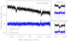 |
Fig. A.1 Left: original 22 GHz spectrum in Arp 220 West (in black), the applied fit to account for the NH3 absorption (red) and the residual spectrum (blue). For clarity purposes the residual spectrum is shown at an offset in y by +25 mJy. Right: zoom into the NH3 (4,2) (top) and NH3 (3,1) (bottom) line features. |
Appendix B: ALMA Band 5 spectrum
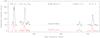 |
Fig. B.1 Spectrum covering all spectral windows observed with ALMA in Band 5. Arp 220 West spectra are artificially offset by 50 mJy for clarity of the figure. The molecular transitions on which each spectral window was centered are indicated above. |
Properties of the additional emission lines securely identified in ALMA Band 5.
All Tables
Properties of the additional emission lines securely identified in ALMA Band 5.
All Figures
|
Fig. 1 Water emission from Arp 220 West (black) and Arp 220 East (red) at 22 (left), 183 (center) and 325 GHz (right). The spectra were extracted from data convolved with the same beam of 0.79′′ × 0.71′′. An artificial offset in intensity was introduced to better show the spectra for each nucleus separately. The dotted lines show the zero-intensity levels. The 22 GHz spectrum has been corrected for contamination by the NH3 (3,1) absorption line. The dark and light blue curves in the 183 and 325 GHz spectra represent the synthetic spectrum used to evaluate the contamination of the water line by other emission lines (Martín et al., in prep.). |
| In the text | |
|
Fig. 2 Maps of the integrated intensity distributions (left) and the velocity fields (right) of the 183 and 325 GHz water lines. Integrated intensity maps: phase center is located at Arp 220 West (α = 15:34:57.220, δ = +23:30:11.60). The contours start at 5σ and are spaced in steps of 10σ (1σ(183 GHz) = 3.9 mJy km s-1, 1σ(325 GHz) = 5.4 mJy km s-1). Velocity fields: color scale is identical for both lines (5200 km s-1–5600 km s-1) and the velocity contours start at 5280 km s-1 and are spaced in steps of 30 km s-1. North is up, east to the left. The beam (0.79′′ × 0.71′′) is indicated in the bottom right corner of each image. The bar in the lower left corner represents a spatial scale of 200 pc. |
| In the text | |
|
Fig. 3 Comparison of the intensities and line shapes between previous single-dish observations (IRAM 30 m, APEX) and spatially smoothed ALMA observations at 183 and 325 GHz. The spectra are in good agreement within the errors imposed by the differences in the sensitivity of the used instruments. |
| In the text | |
|
Fig. 4 Comparison of the line shapes and peak temperatures of the contamination-corrected water spectra at 22 (in green), 183 (blue), and 325 GHz (red) in Arp 220 West (top) and East (bottom). |
| In the text | |
|
Fig. 5 LVG models covering a wide range of physical conditions for three different column densities. For six different kinetic temperatures (TK), the gas temperature variation over a range of H2 densities is shown. The blue, black, and red colors represent the results for the 22, 183, and 325 GHz lines, respectively. Solid lines represent the expected intensities without continuum emission while dashed lines show the results when infrared pumping from dust is taken into account. |
| In the text | |
|
Fig. A.1 Left: original 22 GHz spectrum in Arp 220 West (in black), the applied fit to account for the NH3 absorption (red) and the residual spectrum (blue). For clarity purposes the residual spectrum is shown at an offset in y by +25 mJy. Right: zoom into the NH3 (4,2) (top) and NH3 (3,1) (bottom) line features. |
| In the text | |
|
Fig. B.1 Spectrum covering all spectral windows observed with ALMA in Band 5. Arp 220 West spectra are artificially offset by 50 mJy for clarity of the figure. The molecular transitions on which each spectral window was centered are indicated above. |
| In the text | |
Current usage metrics show cumulative count of Article Views (full-text article views including HTML views, PDF and ePub downloads, according to the available data) and Abstracts Views on Vision4Press platform.
Data correspond to usage on the plateform after 2015. The current usage metrics is available 48-96 hours after online publication and is updated daily on week days.
Initial download of the metrics may take a while.