| Issue |
A&A
Volume 601, May 2017
|
|
|---|---|---|
| Article Number | L2 | |
| Number of page(s) | 4 | |
| Section | Letters | |
| DOI | https://doi.org/10.1051/0004-6361/201730675 | |
| Published online | 21 April 2017 | |
Excitation and evolution of vertically polarised transverse loop oscillations by coronal rain
Department of Physics, University of Warwick, Coventry CV4 7AL, UK
e-mail: This email address is being protected from spambots. You need JavaScript enabled to view it.
Received: 22 February 2017
Accepted: 31 March 2017
Abstract
Context. Coronal rain is composed of cool dense blobs that form in solar coronal loops and are a manifestation of catastrophic cooling linked to thermal instability. The nature and excitation of oscillations associated with coronal rain is not well understood.
Aims. We consider observations of coronal rain in a bid to elucidate the excitation mechanism and evolution of wave characteristics.
Methods. We analyse IRIS and Hinode/SOT observations of an oscillating coronal rain event on the 17th Aug. 2014 and determine the wave characteristics as a function of time using tried and tested time-space analysis techniques.
Results. We exploit the seismological capability of the oscillation to deduce the relative rain mass from the oscillation amplitude. This is consistent with the evolution of the oscillation period showing the loop losing a third of its mass due to falling coronal rain in a 10−15 min time period.
Conclusions. We present the first evidence of the excitation of vertically polarised transverse loop oscillations triggered by catastrophic cooling at the loop top and consistent with two thirds of the loop mass being comprised of cool rain mass.
Key words: Sun: activity / Sun: atmosphere / magnetohydrodynamics (MHD) / Sun: oscillations / instabilities / Sun: UV radiation
© ESO, 2017
1. Introduction
Coronal rain is believed to be associated with catastrophic cooling in coronal plasma in response to localised heating (e.g. Müller et al. 2005; Klimchuk et al. 2008). They are observed in chromospheric and transition region lines as dense blobs of plasma that form near the top of loops and then fall towards the solar surface guided by the magnetic field (Schrijver 2001; De Groof et al. 2004, 2005). Recent observations from the Solar Optical Telescope (SOT) on board Hinode, the Interface Region Imaging Spectrograph (IRIS), and ground-based observatories such as the Swedish Solar Telescope have demonstrated coronal rain is a common occurrence (e.g. Antolin et al. 2010; Antolin & Rouppe van der Voort 2012; Kleint et al. 2014; Antolin et al. 2015; Straus et al. 2015). Coronal rain accelerates towards the solar surface at overall average values of approximately 80 ± 30 m s-2 (Antolin & Rouppe van der Voort 2012), which is considerably smaller than solar gravitational acceleration, even when taking into account the effective gravity in the direction of the guiding magnetic field. Various mechanisms have been proposed to explain this, including plasma pressure effects (Antolin et al. 2010), ponderomotive force when transverse oscillations are present (Verwichte et al. 2017), and the combination of plasma pressure and magnetic tension forces (Mackay & Galsgaard 2001; Kohutova & Verwichte 2017).
Transverse loop oscillations (TLOs) are commonly observed to be polarised in the horizontal direction, reflecting the excitation by a nearby blast wave or large-scale displacement (Aschwanden et al. 1999, 2002; Verwichte et al. 2004). However, there are also examples of vertically polarised TLOs (Wang & Solanki 2004; Mrozek 2011). Correct identification of polarisation is not straightforward as a horizontally polarised TLO seen at the solar limb may appear as an up and down movement in projection. White et al. (2013) observed a vertically polarised TLO in a hot post-flare loop, which was directly connected with the reconnection site below a coronal mass ejection. The excitation mechanism for quiescent coronal loops is unclear. Antolin & Verwichte (2011) showed the presence of transverse oscillations in coronal rain using observations from SOT. Further observational examples from SOT are presented in Verwichte et al. (2017). Kohutova & Verwichte (2016) examined transversely oscillating rain using data from IRIS. These oscillations typically have periods in the order of a few to tens of minutes with projected displacement amplitudes of hundreds of to a thousand km. Antolin & Rouppe van der Voort (2012) has shown that rain is a useful tool for probing the local magnetic field structure. Verwichte et al. (2017) demonstrated that the presence of coronal rain through its concentrated mass may excite transverse loop oscillations and thus provide an additional seismological tool to determine the fraction of the rain mass relative to the total loop mass. This mechanism could explain the excitation of some rain oscillations such as the short-period horizontally polarised TLOs measured by Kohutova & Verwichte (2016). More examples are required to establish whether this type of excitation occurs frequently. In particular, this mechanism could explain vertically polarised TLOs in non-flaring loops without the need for specific external drivers placed below the loop.
2. IRIS and Hinode/SOT observations
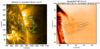 |
Fig. 1 Left: SDO/AIA 171 Å image of the solar East limb with the FOVs of the IRIS and SOT data sets. The data cut used to create the AIA time-distance plots is superimposed. Right: partial FOV of the Hinode/SOT Ca II observation in inverted intensity averaged over 66 consecutive exposures. The two solid lines delineate the data cut across the loop top. The two dashed lines delineate the data cut along the loop. |
We present observations of a coronal loop exhibiting a vertically polarised transverse oscillation in conjunction with coronal rain on the 27th August 2014 seen by IRIS and Hinode/SOT in the time range 08:00−09:30 UT centred at location (950 arcsec E, 200 arcsec N) at the East solar limb (Fig. 1). The IRIS observations are Si IV bandpass slit jaw images at a temporal cadence of 19 s and a spatial pixel size of 0.17 arcsec. The IRIS data has a gap in coverage between 08:49 UT and 09:00 UT. The Hinode/SOT data covers a similar field of view in the Ca II H 3968.5 Å line bandpass at a temporal resolution of 11 s and a spatial pixel size of 0.11 arcsec (2 × 2 binning). We focus on the highlighted loop in Figs. 1 and 2. Using the projected distance of 34.8 arcsec from the loop top to the solar surface as an estimate of the radius of a semi-circular loop, that is, R = 26 ± 5 Mm, a loop length L = 80 ± 20 Mm is found (assumed uncertainty of 20%). We estimate the loop inclination to be θ = 10 ± 10°.
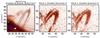 |
Fig. 2 Partial FOV of the IRIS Si IV observations in inverted intensity. Left: image averaged over 40 consecutive exposures. The two solid lines delineate the data cut across the loop top. The two dashed lines delineate the data cut along the loop. Middle and right: observations at two particular times that correspond to a down and up phase of the oscillation. Two parallel lines are provided as fixed reference points. |
From 08:42 UT cold plasma condensations are forming at the loop top that quickly fill up to 60% of the loop length. This is visible in the IRIS data but not in the SOT data because of the higher formation temperature of the Si IV line (around 65 000 K) compared with the Ca II H line (chromospheric). Subsequently, cooler rain is seen falling along the loop legs towards the solar surface in both data sets. At the same time as the condensations form, a fundamental vertically polarised transverse oscillation becomes apparent in the loop, as periodic up and down motions of the condensations seen in Figs. 2 and 3.
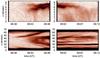 |
Fig. 3 Time-distance cuts perpendicular (top) and parallel (bottom) to the loop axis in the two IRIS data sets in inverted intensity. |
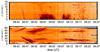 |
Fig. 4 Time-distance plots of the transverse and parallel cuts in the Hinode/SOT data set in inverted intensity. |
The data gap in IRIS does not allow us to observe the transverse oscillation over its entire time span and it is not visible in the SOT data, (see Fig. 4). However, the oscillation is visible over several periods in the time-distance plot before and after the data gap. We employ a tried and tested semi-automated method, illustrated in Fig. 5, to determine the loop top position as a function of time (Verwichte et al. 2004, 2009). The time-distance plot is filtered using a two-dimensional continuous Mexican Hat wavelet transform to remove linear background trends in intensity to enhance the loop contrast (Witkin 1983; White & Verwichte 2012). The loop top position is first estimated by eye, which serves at each instance as the initial guess for the fitting of a Gaussian profile to the filtered loop profile. The half-width of the fitted Gaussian is taken to be the one-sigma error in position. The loop top displacement is found by subtracting a linear fit from the position time series.
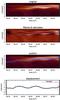 |
Fig. 5 Procedure of measuring the transverse loop displacement as a function of time, for the first IRIS time period. Top: the original time-distance plot. Second: the wavelet-filtered plot with the estimated loop position superimposed. The section above the red dashed line has been used for measuring the loop position. Third: the measured loop displacement based on Gaussian fitting of the loop cross-section at each time. The light dashed lines are error estimates based on the half-width of the Gaussian profile. Bottom: the loop displacement as a function of time, achieved by subtracting a linear fit from the position. Colour represents the strength of the fit based on ridge strength. |
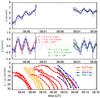 |
Fig. 6 Top: loop position obtained from IRIS as a function of time. The error bars correspond to the half-width of a Gaussian profile fitted to the loop cross-section at each time. The dashed lines are linear fits to each time series. Middle: loop displacement as a function of time obtained by subtracting the linear profile from the loop position time series. The red and green curves are fitted sinusoidal curves with the corresponding parameters listed. Bottom: position of individual rain blobs as distance relative to the approximate loop top x0, as a function of time. |
Once the displacement time series have been found, a sinusoidal curve of the form ξ(t) = ξ0 cos(2πt/P + φ0) is fitted to the time series using a Levenberg-Marquardt algorithm, where ξ0 is the displacement amplitude, P is the oscillation period, and φ0 is the oscillation phase at the reference time t0 = 07:58:30 UT (see Fig. 6). For the time series before the data gap we find ξ0,1 = 0.3 ± 0.1 arcsec = 0.22 ± 0.07 Mm, and P1 = 2.6 ± 0.1 min. For the time series after the data gap we find ξ0,2 = 0.2 ± 0.1 arcsec = 0.15 ± 0.07 Mm, and P2 = 2.1 ± 0.1 min. The ratio of periods is equal to P2/P1 = 0.81 ± 0.07. If the oscillation is a fundamental standing mode, the phase speeds for both times are found to be Vph = 1050 ± 250 km s-1 and 1300 ± 300 km s-1, respectively. The displacement amplitude ξ0,2 is only a third less than ξ0,1, which indicates that the excitation of the oscillation is prolonged in time rather than instantaneous. TLOs that are excited impulsively are expected to damp quickly due to resonant absorption (Aschwanden et al. 2002; Ruderman & Roberts 2002).
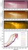 |
Fig. 7 Time-distance plots of the transverse cuts in the SDO/AIA 211 Å, 193 Å, and 171 Å bandpasses, respectively. The top of the loop as seen in IRIS is at x = 15−20 arcsec where the intensity enhancement is visible in 171 Å. Bottom: intensity averaged across the data cut for each AIA bandpass, interpolated along the track highlighted in the 171 Å bandpass, as a function of time, normalised with respect to their peak value. |
The IRIS and SOT data sets are complemented with observations from SDO/AIA. Although the spatial resolution of 0.62 arcsec pixel size does not allow us to observe the same oscillation directly, other features are of interest, as is summarised in Fig. 7. Firstly, there is evidence of TLOs in overlying loop in the coronal bandpasses of SDO/AIA, notably 171 Å and 193 Å. Those oscillations have similar periods but much larger displacement amplitudes of approximately 3 arcsec. Secondly, there is a pattern of intensity increase as a function of time in the different bandpasses that agrees with an evolution from high to low temperatures, expected from cooling. Figure 8 shows the differential emission measure curves at various times extracted from the AIA intensities along the track in Fig. 7 using the method outlined in Hannah & Kontar (2012). The initial intensity has been assumed to be a proxy for the line-of-sight background intensity and has been subtracted from the intensity at other times. The emission increases with time and a second hotter component centred around 1.9 MK develops. Figure 8 also shows elements of a thermal cycle in the evolution of the average temperature and number density. We recognise the heating phase between 08:10 and 08:20 UT followed by a condensation phase between 08:20 and 08:45 UT. The plasma becomes visible in the IRIS bandpass at a peak temperature of 0.065 MK from 08:43 UT. The evacuation phase follows from 08:45, as evident from the falling rain seen by SOT.
3. Discussion
Verwichte et al. (2017) found that for a vertically polarised transverse oscillation to be excited by a concentrated coronal rain blob, an approximate expression that relates the oscillation displacement amplitude to the coronal rain mass is: 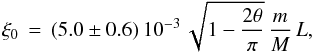 (1)where θ is the inclination angle of the loop plane with respect to the photospheric normal, and m/M is the fraction of coronal rain mass relative to the total loop mass. The values found for ξ0,1, ξ0,2, θ and L are inserted into Eq. (1) and the mass ratios at the two time intervals are found to be
 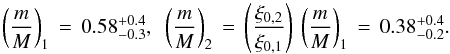 (2)The value of m/M = 0.58 at the start of the event is consistent with the large amount of coronal rain that had formed simultaneously at that time along a 60% fraction of the loop length. This result is similar to what had been found to explain the short-period horizontally polarised transverse oscillations by Kohutova & Verwichte (2016). Antolin et al. (2015) had shown that in some cases coronal rain may make up most of the loop’s mass. Equation (2) also shows that towards the end of the visible oscillation, the fraction of rain mass has dropped down to 40%.
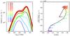 |
Fig. 8 Left: differential emission measure as a function of temperature determined from the AIA intensities along the track shown in Fig. 7. The initial intensity has been assumed to be the background intensity and has been subtracted. The dashed curve is a two-Gaussian fit. Right: electron number density, assuming a 10 Mm line-of-sight depth, as a function of EM-weighted average temperature over the interval 5.5 ≤ log T ≤ 6.5. |
The evolution of period independently holds information on the rain mass. If we interpret the oscillation to be a (Alfvénic) kink mode, the period of oscillation is proportional to the square root of the internal loop density. Then, ρ0,2/ρ0,1 = (P2/P1)2 = 0.65 ± 0.1. With the crude assumption that the density varies simultaneously everywhere in the loop, it is found that over a 10−15 min time period the loop has lost a third of its mass due to falling rain. Indeed, from Fig. 4 we see that between 08:45 UT and 09:00 UT substantial rain is moving down both loop legs. For a constant loop volume M2/M1 = (P2/P1)2 = 0.65 ± 0.1, this change is solely in rain mass. We combine Eq. (2) with the relations following from an assumption of constant hot plasma mass, that is,  and mplasma = M1−m1 = M2−m2, to find an alternate expression for (m/M)2:
 ![Mathematical equation: \begin{equation} \left(\frac{m}{M}\right)_2 \,=\, 1 - \left(\frac{P_1}{P_2}\right)^2\left[1 - \left(\frac{m}{M}\right)_1\right] \,=\, 0.34^{+0.7}_{-0.2} . \end{equation}](/articles/aa/full_html/2017/05/aa30675-17/aa30675-17-eq38.png) (3)This result independently confirms the value found in Eq. (2). Alternatively, the two rain mass relations are combined as
(3)This result independently confirms the value found in Eq. (2). Alternatively, the two rain mass relations are combined as 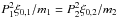 equal to a constant that depends on loop length, inclination, initial total mass and magnetic field strength.
The cut along the loop in Fig. 3 shows, in the time period from before 09:00 UT until 09:10 UT at position 40 arcsec to 60 arcsec along the loop, evidence of rain blobs falling in a regular repetition resembling the periodicity of the transverse oscillation. They are highlighted as blue tracks in Fig. 6. We have established a link between change in oscillation period and down flows but evidence of a link between individual rain events and oscillation phase is more difficult to ascertain. Assuming this periodicity is real and not due to limited instrumental resolution, we consider two likely explanations. First, if the cool plasma is contained at the loop top in a shallow dip, a superimposed vertical TLO displaces the loop position radially, and periodically removes the dip to allow cool material to fall down the legs. Second, the oscillation causes small perturbations to the critical state of the loop which trigger further catastrophic cooling events with the same periodicity.
In conclusion, we have found the first evidence of the excitation of a small-amplitude vertically polarised transverse oscillation during catastrophic cooling in the top of a loop leading to coronal rain. The nature of the excitation is extended in time leading to a “decay-less” oscillation. We have demonstrated that the evolution of the oscillation amplitude and period independently show that the cool rain mass evolves from 60% to 40% of the total loop mass. One-third of the loop mass is lost due to coronal rain falling along the loop legs. Decay-less oscillations with similar periods are observed in the over-arching coronal loops, before and during the rain event, similar in appearance to those reported by (e.g. Wang et al. 2012; Nisticò et al. 2013). This suggests that, rather than continuous footpoint driving or leaky sunspot oscillations (Nisticò et al. 2013), their manifestation may be connected with the catastrophic cooling process (Chin et al. 2010). Further MHD simulations will be presented in future that explore the range of validity of Eq. (1).
Acknowledgments
E.V. acknowledges support from the Warwick STFC Consolidated Grant ST/L000733/I. P.K. acknowledges the support of the UK STFC Ph.D. studentship. We thank P. Antolin and G. Vissers, co-observers during the August 2014 observing campaign at the Swedish Solar Telescope, coordinated with IRIS/Hinode (IHOP 262). IRIS is a NASA small explorer mission developed and operated by LMSAL with contributions from NASA Ames Research Center and the NSC (Norway). Hinode is a Japanese mission developed and launched by ISAS/JAXA, partnered with NAOJ, NASA and STFC (UK), in cooperation with ESA and NSC (Norway). This research has made use of SunPy, an open-source and free community-developed solar data analysis package written in Python (http://sunpy.org). We acknowledge the referee’s constructive input.
References
- Antolin, P., & Rouppe van der Voort, L. 2012, ApJ, 745, 152 [NASA ADS] [CrossRef] [Google Scholar]
- Antolin, P., & Verwichte, E. 2011, ApJ, 736, 121 [NASA ADS] [CrossRef] [Google Scholar]
- Antolin, P., Shibata, K., & Vissers, G. 2010, ApJ, 716, 154 [NASA ADS] [CrossRef] [Google Scholar]
- Antolin, P., Vissers, G., Pereira, T. M. D., Rouppe van der Voort, L., & Scullion, E. 2015, ApJ, 806, 81 [NASA ADS] [CrossRef] [Google Scholar]
- Aschwanden, M. J., Fletcher, L., Schrijver, C. J., & Alexander, D. 1999, ApJ, 520, 880 [NASA ADS] [CrossRef] [Google Scholar]
- Aschwanden, M. J., de Pontieu, B., Schrijver, C. J., & Title, A. M. 2002, Sol. Phys., 206, 99 [NASA ADS] [CrossRef] [Google Scholar]
- Chin, R., Verwichte, E., Rowlands, G., & Nakariakov, V. M. 2010, Phys. Plasmas, 17, 032107 [NASA ADS] [CrossRef] [Google Scholar]
- De Groof, A., Berghmans, D., van Driel-Gesztelyi, L., & Poedts, S. 2004, A&A, 415, 1141 [NASA ADS] [CrossRef] [EDP Sciences] [Google Scholar]
- De Groof, A., Bastiaensen, C., Müller, D. A. N., Berghmans, D., & Poedts, S. 2005, A&A, 443, 319 [NASA ADS] [CrossRef] [EDP Sciences] [Google Scholar]
- Hannah, I. G., & Kontar, E. P. 2012, A&A, 539, A146 [NASA ADS] [CrossRef] [EDP Sciences] [Google Scholar]
- Kleint, L., Antolin, P., Tian, H., et al. 2014, ApJ, 789, L42 [NASA ADS] [CrossRef] [Google Scholar]
- Klimchuk, J. A., Patsourakos, S., & Cargill, P. J. 2008, ApJ, 682, 1351 [Google Scholar]
- Kohutova, P., & Verwichte, E. 2016, ApJ, 827, 39 [NASA ADS] [CrossRef] [Google Scholar]
- Kohutova, P., & Verwichte, E. 2017, A&A, in press, DOI: 10.1051/0004-6361/201629912 [Google Scholar]
- Mackay, D. H., & Galsgaard, K. 2001, Sol. Phys., 198, 289 [NASA ADS] [CrossRef] [Google Scholar]
- Mrozek, T. 2011, Sol. Phys., 270, 191 [NASA ADS] [CrossRef] [Google Scholar]
- Müller, D. A. N., De Groof, A., Hansteen, V. H., & Peter, H. 2005, A&A, 436, 1067 [NASA ADS] [CrossRef] [EDP Sciences] [Google Scholar]
- Nisticò, G., Nakariakov, V. M., & Verwichte, E. 2013, A&A, 552, A57 [NASA ADS] [CrossRef] [EDP Sciences] [Google Scholar]
- Ruderman, M. S., & Roberts, B. 2002, ApJ, 577, 475 [NASA ADS] [CrossRef] [Google Scholar]
- Schrijver, C. J. 2001, Sol. Phys., 198, 325 [NASA ADS] [CrossRef] [Google Scholar]
- Straus, T., Fleck, B., & Andretta, V. 2015, A&A, 582, A116 [NASA ADS] [CrossRef] [EDP Sciences] [Google Scholar]
- Verwichte, E., Nakariakov, V. M., Ofman, L., & Deluca, E. E. 2004, Sol. Phys., 223, 77 [NASA ADS] [CrossRef] [Google Scholar]
- Verwichte, E., Aschwanden, M. J., Van Doorsselaere, T., Foullon, C., & Nakariakov, V. M. 2009, ApJ, 698, 397 [NASA ADS] [CrossRef] [Google Scholar]
- Verwichte, E., Antolin, P., Rowlands, G., Kohutova, P., & Neukirch, T. 2017, A&A, 598, A57 [NASA ADS] [CrossRef] [EDP Sciences] [Google Scholar]
- Wang, T. J., & Solanki, S. K. 2004, A&A, 421, L33 [NASA ADS] [CrossRef] [EDP Sciences] [Google Scholar]
- Wang, T., Ofman, L., Davila, J. M., & Su, Y. 2012, ApJ, 751, L27 [Google Scholar]
- White, R. S., & Verwichte, E. 2012, A&A, 537, A49 [NASA ADS] [CrossRef] [EDP Sciences] [Google Scholar]
- White, R. S., Verwichte, E., & Foullon, C. 2013, ApJ, 774, 104 [NASA ADS] [CrossRef] [Google Scholar]
- Witkin, A. 1983, in Proc. 8th Int. Joint Conf. Artificial Intell., ed. A. Bundy, 2, 1019 [Google Scholar]
All Figures
|
Fig. 1 Left: SDO/AIA 171 Å image of the solar East limb with the FOVs of the IRIS and SOT data sets. The data cut used to create the AIA time-distance plots is superimposed. Right: partial FOV of the Hinode/SOT Ca II observation in inverted intensity averaged over 66 consecutive exposures. The two solid lines delineate the data cut across the loop top. The two dashed lines delineate the data cut along the loop. |
| In the text | |
|
Fig. 2 Partial FOV of the IRIS Si IV observations in inverted intensity. Left: image averaged over 40 consecutive exposures. The two solid lines delineate the data cut across the loop top. The two dashed lines delineate the data cut along the loop. Middle and right: observations at two particular times that correspond to a down and up phase of the oscillation. Two parallel lines are provided as fixed reference points. |
| In the text | |
|
Fig. 3 Time-distance cuts perpendicular (top) and parallel (bottom) to the loop axis in the two IRIS data sets in inverted intensity. |
| In the text | |
|
Fig. 4 Time-distance plots of the transverse and parallel cuts in the Hinode/SOT data set in inverted intensity. |
| In the text | |
|
Fig. 5 Procedure of measuring the transverse loop displacement as a function of time, for the first IRIS time period. Top: the original time-distance plot. Second: the wavelet-filtered plot with the estimated loop position superimposed. The section above the red dashed line has been used for measuring the loop position. Third: the measured loop displacement based on Gaussian fitting of the loop cross-section at each time. The light dashed lines are error estimates based on the half-width of the Gaussian profile. Bottom: the loop displacement as a function of time, achieved by subtracting a linear fit from the position. Colour represents the strength of the fit based on ridge strength. |
| In the text | |
|
Fig. 6 Top: loop position obtained from IRIS as a function of time. The error bars correspond to the half-width of a Gaussian profile fitted to the loop cross-section at each time. The dashed lines are linear fits to each time series. Middle: loop displacement as a function of time obtained by subtracting the linear profile from the loop position time series. The red and green curves are fitted sinusoidal curves with the corresponding parameters listed. Bottom: position of individual rain blobs as distance relative to the approximate loop top x0, as a function of time. |
| In the text | |
|
Fig. 7 Time-distance plots of the transverse cuts in the SDO/AIA 211 Å, 193 Å, and 171 Å bandpasses, respectively. The top of the loop as seen in IRIS is at x = 15−20 arcsec where the intensity enhancement is visible in 171 Å. Bottom: intensity averaged across the data cut for each AIA bandpass, interpolated along the track highlighted in the 171 Å bandpass, as a function of time, normalised with respect to their peak value. |
| In the text | |
|
Fig. 8 Left: differential emission measure as a function of temperature determined from the AIA intensities along the track shown in Fig. 7. The initial intensity has been assumed to be the background intensity and has been subtracted. The dashed curve is a two-Gaussian fit. Right: electron number density, assuming a 10 Mm line-of-sight depth, as a function of EM-weighted average temperature over the interval 5.5 ≤ log T ≤ 6.5. |
| In the text | |
Current usage metrics show cumulative count of Article Views (full-text article views including HTML views, PDF and ePub downloads, according to the available data) and Abstracts Views on Vision4Press platform.
Data correspond to usage on the plateform after 2015. The current usage metrics is available 48-96 hours after online publication and is updated daily on week days.
Initial download of the metrics may take a while.