| Issue |
A&A
Volume 601, May 2017
|
|
|---|---|---|
| Article Number | A119 | |
| Number of page(s) | 25 | |
| Section | Stellar atmospheres | |
| DOI | https://doi.org/10.1051/0004-6361/201629854 | |
| Published online | 15 May 2017 | |
An abundance analysis from the STIS-HST UV spectrum of the non-magnetic Bp star HR 6000
1 Istituto Nazionale di Astrofisica, Osservatorio Astronomico di Trieste, via Tiepolo 11, 34143 Trieste, Italy
e-mail: This email address is being protected from spambots. You need JavaScript enabled to view it.
2 Department of Astronomy, University of Michigan, Ann Arbor, MI 48109-1042, USA
3 Center for Astrophysics and Space Astronomy, University of Colorado, Boulder, CO 80309-0389, USA
4 Istituto Nazionale di Astrofisica, Osservatorio Astronomico di Catania, via S. Sofia 78, 95123 Catania, Italy
5 Universita’ di Catania, Dipartimento di Fisica e Astronomia, Sezione Astrofisica, via S. Sofia 78, 95123 Catania, Italy
Received: 6 October 2016
Accepted: 6 December 2016
Abstract
Context. The sharp-line spectrum of the non-magnetic, main-sequence Bp star HR 6000 has peculiarities that distinguish it from those of the HgMn stars with which it is sometimes associated. The position of the star close to the center of the Lupus 3 molecular cloud, whose estimated age is on the order of 9.1 ± 2.1 Myr, has lead to the hypothesis that the anomalous peculiarities of HR 6000 can be explained by the young age of the star.
Aims. Observational material from the Hubble Space Telescope (HST) provides the opportunity to extend the abundance analysis previously performed for the optical region and clarify the properties of this remarkable peculiar star. Our aim was to obtain the atmospheric abundances for all the elements observed in a broad region from 1250 to 10 000 Å.
Methods. An LTE synthetic spectrum was compared with a high-resolution spectrum observed with the Space Telescope Imaging Spectrograph (STIS) equipment in the 1250−3040 Å interval. Abundances were changed until the synthetic spectrum fit the observed spectrum. The assumed model is an LTE, plane-parallel, line-blanketed ATLAS12 model already used for the abundance analysis of a high-resolution optical spectrum observed at ESO with the Ultraviolet and Visual Echelle Spectrograph (UVES). The stellar parameters are Teff = 13450 K, log g = 4.3, and zero microturbulent velocity.
Results. Abundances for 28 elements and 7 upper limits were derived from the ultraviolet spectrum. Adding results from previous work, we have now quantitative results for 37 elements, some of which show striking contrasts with those of a broad sample of HgMn stars. The analysis has pointed out numerous abundance anomalies, such as ionization anomalies and line-to-line variation in the derived abundances, in particular for silicon. The inferred discrepancies could be explained by non-LTE effects and with the occurrence of diffusion and vertical abundance stratification. In the framework of the last hypothesis, we obtained, by means of trial and error, empirical step functions of abundance versus optical depth log (τ5000) for carbon, nitrogen, silicon, manganese, and gold, while we failed to find such a function for phosphorous. The poor results for carbon, and mostly for phosphorus, suggest the possible importance in this star of NLTE effects to be investigated in future works.
Key words: stars: abundances / stars: atmospheres / stars: chemically peculiar / stars: individual: HR 6000
© ESO, 2017
1. Introduction
The ASTRAL spectral library for hot stars (Ayres et al. 2014) includes observations of the peculiar star HR 6000 (HD 144667), giving us the possibility of studying at high resolution the ultraviolet spectrum of this special peculiar star for the first time after the International Ultraviolet Explorer (IUE) era. The star is anomalous because it does not fit into any of the typical CP subclasses, but seems to combine abundance anomalies from several Bp subtypes (Andersen et al. 1984). A remarkable characteristic is the extreme deficiency of silicon, which makes HR 6000 the most deficient silicon star of the HgMn group, with which it is usually associated.
Peculiarities in the spectrum of HR 6000 were first noted by Bessell & Eggen (1972), who classified it as a peculiar main-sequence B star with strong P ii lines and weak helium (see also van den Ancker et al. 1996). This star is the brighter, more massive component of the visual binary system Δ199 or Dunlop 199 (Dunlop 1829). The second component is the Herbig Ae star HR 5999 (HD 144668) (Eggen 1975). Because the Δ199 double system is located close to the center of the Lupus 3 molecular cloud, which is populated by numerous TTauri stars, it has been assumed that the system is the same age as the cloud, i.e., about (9.1 ± 2.1) Myr (James et al. 2006). In this case, HR 6000 is a very young peculiar star and its anomalous peculiarity could be explained by its young age. The spectrum of HR 6000 also seems to be polluted by lines of some cool star. The identification of an unshifted Li i line at 6707.7 Å led Castelli & Hubrig (2007) to support the hypothesis from van den Ancker et al. (1996) of the presence of a faint TTauri companion, which could be either physically related to HR 6000 to form a close binary system or located in the foreground of HR 6000.
After recognition of its peculiar nature, the first high-resolution studies of the chemical composition of HR 6000 were of an ultraviolet spectrum obtained with IUE in the far and near ultraviolet on March 1979 (Castelli et al. 1981, 1985) and an optical spectrum observed at ESO with a dispersion of 12 Å mm-1 covering the spectral range λλ 3323−5316 Å (Andersen & Jaschek 1984).
While very significant qualitative results on the nature of the star were provided from the optical spectra by Andersen et al. (1984), the quantitative analysis from the IUE spectra (Castelli et al. 1985) has given abundances for almost all the elements observed in the IUE range (1258−1960 Å and 2050−3150 Å), but with large uncertainties. The quantitative analysis of the IUE spectra was a very difficult task, in particular owing to the rather low resolving power and poor signal-to-noise ratio (S/N), severe line crowding, and poor quality of the line lists available at that time for computing synthetic spectra. However, the underabundance of several elements (Be, C, N, Mg, Al, Si, S, Sc, Co, Ni, Cu, and Zn) and overabundance of others elements (B, P, Ca, Mn, Fe, and Ga) were determined. For a few elements, spurious high abundances were assigned owing to several unresolved blended features and unidentified components.
Later on, in a series of papers, Smith (1993, 1994, 1997) and Smith & Dworetsky (1993) published the abundances of selected elements obtained from IUE spectra of a sample of HgMn stars, including HR 6000, which they noted did not fit the typical abundance pattern. They pointed out three additional stars, 33 Gem, 36 Lyn, and 46 Aql, with abundances that depart from the more general behavior observed in the majority of the HgMn class members.
A comparison of the Smith and Smith & Dworetsky results with those from Castelli et al. (1985) for the elements in common (Mg ii, Cr ii, Mn ii, Fe ii, Ni ii, Zn ii) has shown agreement within the error limits for all the elements except for Zn ii whose abundance was estimated −8.3 dex by Castelli et al. (1985) and −9.2 dex by Smith (1994). We currently adopt an upper limit of −8.84 for Zn.
Several years later, high-resolution optical spectra became available to study HR 6000 in the visual range. Catanzaro et al. (2004) analyzed the 3800−7000 Å region on FEROS spectra observed with 48 000 resolving power, while Castelli & Hubrig (2007) and Castelli et al. (2009) studied the 3040−10 000 Å region on a spectrum observed at ESO with the Ultraviolet and Visual Echelle Spectrograph (UVES) at a resolving power ranging from 80 000 to 110 000. The comparison of the abundances derived from the FEROS and UVES spectra were in rather good agreement, with discrepancies larger than 0.3 dex only for He i, Mg ii, and Mn ii. For iron the difference was 0.3 dex. In both analyses there are only upper limits for a few elements. Discordant abundances from the visual and ultraviolet spectra were found for O i, S ii, and Ti ii. In Castelli & Hubrig (2007) several studies on the nature of the star are quoted, included those on variability. While a weak photometric variability was pointed out by van den Ancker et al. (1996) and by Kurtz & Marang (1995), no spectroscopic variability was evident from the different spectra taken by Andersen & Jaschek (1984) and Castelli & Hubrig (2007) at different epochs and with different instruments.
The Space Telescope Imaging Spectrograph (STIS) ultraviolet spectrum of the ASTRAL library gives us the opportunity to extend the UVES observations to the ultraviolet and supersede the low quality IUE data. The entire range from 1250 to 10 000 Å is now covered by high-resolution spectra of HR 6000. The presence of elements not observed in the optical region and elements that are present in the ultraviolet with more ionization states and more lines allow us to improve the investigation of effects related to the atomic diffusion (Michaud 1970), in particular, vertical abundance stratification.
The first theoretical attempt to point out the effect of abundance stratification on line profiles is from Alecian & Artru (1988) who analyzed the case of the Ga ii resonance line at 1414.401 Å in the atmospheres of Ap stars. Babel (1994) explained the Ca ii profile at 3933 Å observed in Ap stars with the help of a step function of the calcium abundance versus optical depth. Leone & Lanzafame (1997) and Leone (1998) introduced the use of the contribution functions to associate abundances with atmospheric layers. In addition, Leone et al. (1997) and Catanzaro et al. (2016) extended the search for vertical abundance stratification to the ultraviolet.
All the previous studies tell us that in peculiar stars with low rotational velocity and no convective motions, such as in HR 6000, vertical abundance stratification for certain elements may be present near the surface. Currently several studies have been performed with the aim of detecting vertical stratification of the abundances. In this context, of particular interest is the VeSE1kA project (LeBlanc et al. 2015). This paper could add some more information related to the abundance peculiarities observed in HgMn stars.
2. Observations
HR 6000 is one of the targets included in the Hot Stars part of the HST Cycle 21 “Advanced Spectral Library (ASTRAL)” Project (Ayres et al. 2014: GO-13346). The star was observed several days in October 2014 with moderate and high-resolution echelle settings of STIS. The final spectrum covers the range 1150−3045 Å. The nominal resolving power R ranges from about 30 000 to 110 000; the S/N typically is greater than 100, approaching 200 in selected regions. We used the final spectrum that resulted from the calibration and merging of the overlapping echelle spectra observed in the different wavelength intervals, as performed by the ASTRAL Science Team1.
For this work we analyzed the whole region from 1250 to 3045 Å, using the IRAF tool “continuum” to normalize the observed spectrum to the continuum level. When we compared observed and computed spectra, we tentatively fixed different resolving powers for the different intervals corresponding roughly to major switches in the echelle modes. While the theoretical resolving powers of the moderate-resolution far-ultraviolet E140M and moderate-resolution near-UV E230M echelle modes are 45 000 and 30 000, respectively (Ayres 2010), measurements of narrow features in the HR 6000 spectrum suggest lower effective resolutions of 30 000 and 25 000, respectively. However, at the longer wavelengths (>2300 Å) recorded with the NUV high-resolution echelle E230H, there appears to be little degradation of the theoretical resolving power of 110 000. The cause of the resolution decrease for the medium-resolution spectra is unknown, but currently is under investigation. The wavelength scale of the STIS spectra are provided in vacuum for the whole observed region. We converted the wavelength scale of the final spectrum from vacuum to air for the 2000−3040 Å interval.
3. The analysis
Abundances were determined with the synthetic spectrum method by changing the abundance of a given element until agreement between observed and computed profiles is obtained. We used the SYNTHE code (Kurucz 2005) to compute local thermodynamic equilibrium (LTE) synthetic spectra when the adopted abundance is constant with depth and a modified version of SYNTHE (Kurucz, priv. comm.) when a vertical abundance stratification is considered for a given element. To be consistent with a previous abundance analysis performed on an UVES optical spectrum by Castelli et al. (2009), we adopted the same model atmosphere without any modification. It is a plane-parallel, LTE model atmosphere with parameters Teff = 13 450 K, log g = 4.3, and microturbulent velocity ξ = 0.0 km s-1, computed with the ATLAS12 code (Kurucz 2005) for the individual abundances of HR 6000, as derived from the optical spectrum and tabulated in Castelli et al. (2009). In all the computations the continuous opacity includes the scattering contribution from electron scattering and Rayleigh scattering from neutral hydrogen, neutral helium, and molecular hydrogen H2. Hydrogen Rayleigh scattering, which is an important opacity source for modeling Lymanα wings, was computed according to Gavrila (1967). The other scattering sources are described in Kurucz (1970). No scattering was considered in the line source function, which was approximated with the Planck function.
The model parameters are updated values from those derived by Castelli & Hubrig (2007) from both Balmer profiles and the Fe i and Fe ii ionization equilibrium. In Castelli et al. (2009)Teff and log g were obtained from Strömgren photometry, from the requirement that there is no correlation between the Fe ii abundances derived from high- and low-excitation lines, and from the constraint of Fe i−Fe ii ionization equilibrium. The only element used to fix the model parameters was iron because other elements were not observed in different ionization degrees in the optical spectrum, except for phosphorous, which was present with P ii and P iii lines. Owing to the larger number of lines and more trustworthy atomic data for both Fe i and Fe ii lines than for phosphorous, in particular P iii, we preferred to use iron to phosphorous for the determination of the model parameters.
As discussed in Castelli et al. (2009), the Balmer lines were no longer used owing to the several problems related with the UVES spectra in the regions of the Balmer lines.
The computed spectrum was broadened for a rotational velocity vsini = 1.5 km s-1 and a Gaussian instrumental profile corresponding to different resolving powers for different intervals, as indicated in Sect. 2. In order to superimpose the observed profiles on the computed profiles the observed spectrum was shifted by a velocity ranging from 0.0 km s-1 at 1250 Å to 2.0 km s-1 at 3040 Å.
3.1. The line lists
To compute the synthetic spectrum we adopted as main line list the file gfall05jun16.dat, available on the Kurucz website on June 2016 (Kurucz 2016, K16)2. All the lines arising from observed levels of elements from hydrogen to zinc up to six or more ionization degrees are listed with wavelength, log gf value, excitation potential of upper and lower levels and broadening parameters. The log gf values are taken from the literature, mostly when experimental data are available, otherwise the values are those computed by Kurucz with a semi-empirical method.
The list also includes lines of Fe ii (Castelli & Kurucz 2010), Fe i (Peterson & Kurucz 2015), and Mn ii (Castelli et al. 2015) observed in high-resolution stellar spectra but neither measured or classified in laboratory work. They arise from energy levels predicted (approximately) by the theory. The method takes note of coincidences of unidentified stellar spectral lines with the lines arising from a given predicted energy level. After an appropriate energy shift (correction) of the levels, the lines may be considered to be identified, and used in spectral synthesis.
For elements heavier than zinc the Kurucz line lists contain lines taken from the literature. They are mostly lines of neutral and first ionized atoms.
We changed and implemented the line data in the Kurucz line list. The big file gfall05jun16.dat was divided into several smaller files that we then modified. The main changes were made on Cr ii, Cr iii, Mn ii, Mn iii, and Fe ii. For numerous lines of Cr ii and Fe ii, the Kurucz log gf values were replaced by those given in the Fe ii and Cr ii line lists from Raassen & Uylings (1998), which were available some time ago on a website cited by the authors, but it is no longer online. We changed a log gf value from Kurucz only when that from Raassen & Uylings (1998) improved the agreement between the observed and computed spectra. For a few Cr iii lines and several Mn ii and Mn iii lines we lowered the Kurucz log gf value when it gave rise to a very strong computed, but unobserved line. We checked these changes by comparing synthetic spectra of the HgMn star HD 175640 and of the normal star ι Her with their STIS spectra.
For other elements we modified the Kurucz line lists by using data taken from the atomic database (version 5)3 (Kramida et al. 2015) of the National Institute of Standards and Technology (NIST), or from more recent literature. We both modified several log gf values and added lines for Ga i, Ga ii, Ge ii, Zr ii, Ru ii, Rh ii, Pd ii, Ag ii, Cd ii, Sn ii, Os ii, Ir ii, Hg i, and Hg ii. For In ii we only replaced by the NIST values the atomic data of the Kurucz line list for the 1250−3000 Å region. We added lines of Ga iii, As ii, Y iii, Zr iii, Xe i, Xe ii, Yb iii, Pt ii, Pt iii, Au ii, Au iii, Hg iii, and Tl ii. At the moment these ions are left out of the Kurucz line list. References for the modified or added log gf sources of the ions relevant for this paper are given in Table 1. The complete modified list may be obtained at the Castelli’s website4.
log gf sources for the heavy elements relevant for this paper.
3.2. The abundances
A short description of the elements observed in the ultraviolet spectrum of HR 6000 together with a list of the analyzed lines with the atomic data and the corresponding abundances is given in Appendix A. The average abundance for each element is given in Col. 6 of Table 2, which also displays in successive columns the abundances for HR 6000 determined from spectra observed with different instruments in different ranges and by different researchers, as described in the Introduction. Column 2 of Table 2 lists the abundances derived from the IUE spectra by Castelli et al. (1985, CCHM85) and Col. 3 those obtained from IUE spectra by Smith & Dworetsky (1993, SD) and Smith (1993; 1994; 1997, S). Columns 4 and 5 list the abundances derived from the optical spectra by Catanzaro et al. (2004, CLD04) and by Castelli et al. (2009, CKH). In Col. 6 the abundances obtained in this paper from the STIS spectrum are given (CCACL16). The final abundances from both UVES and STIS spectra are collected in Col. 7. Columns 8 and 9 list the solar abundances from Asplund et al. (2009), Scott et al. (2015a,b), and Grevesse et al. (2015) and their differences with the HR 6000 abundances. Advancing from Cols. 2 to 7 one can note the increasing number of elements for which abundances became available with time and the decreasing number of upper limits.
In addition to the non-solar abundances for almost all the observed elements, we point out two other types of abundance anomalies as follows:
-
1.
Ionization anomalies, i.e., LTE abundances for some elementsthat are markedly inconsistent among different ionization states.The most significant abundance differences are pointed out inTable 3.
-
2.
The considerable line-to-line variation in the derived abundances for C i, N i, Al ii, Si ii, Si iii, Cl i, Ti iii, Mn iii, Sn ii, and Au ii. The large scatter in the abundances can be inferred from the large mean square error associated with the final average abundance listed in Col. 7 of Table 2 for the considered ion.
Abundances log (Nelem/Ntot) in HR 6000 from different studies.
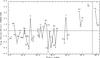 |
Fig. 1 Differences between the abundance from a selected ion of a given element in HR 6000 and the solar abundance, as they are listed in Col. 3 of Table 4. The arrow for Na, Cl, Co, Zn, Ge, Sr, and Zr indicates an upper abundance limit. The vertical full line indicates the jump from Z = 57 to Z = 77, a range in atomic numbers for which no elements were observed in HR 6000. The errors can be inferred from Col. 1 of Table 4. |
In the final spectrum synthesis calculation, it was necessary to adopt single abundances for elements with different abundances for different ionization stages. This is also needed for abundance comparisons with other stars such as in Table 4. For the light and heavy elements we chose the abundances of the dominant ionization state, except for silicon for which we preferred to adopt the value −7.35 dex obtained from the Si ii lines at 3862.595, 4128.074, and 4130.894 Å. For the iron-group elements we adopted the abundances derived from the first ionization state, if observed, because the log gf values available for this state are usually more critically evaluated than those for the second ionization degree. The difference of these abundances with respect to the solar values are listed in Col. 3 of Table 4 and are plotted in Fig. 1. Upper limits for Na, Cl, Co, Zn, Ge, Sr, and Zr are indicated with an arrow. The figure shows a tendency for the elements from He to Zr to be more or less depleted relative to the Sun, except for Be, P, Ti,Cr, Mn, Fe, Ga, and Y. Instead, the observed heavy elements with atomic number Z≥ 50 are overabundant, in particular Cd, Xe, and Au, which show enhancements from 3 to 4 orders of magnitude.
The adopted abundances were used to compare the chemical composition of HR 6000 with that of other HgMn stars. Ghazaryan & Alecian (2016) presented a compilation of the abundances taken from the most recent literature for a sample of 104 HgMn stars. Table 4 compares the over- and underabundances of HR 6000 with the minimum and maximum abundances of a given element from the Ghazaryan & Alecian (2016) compilation. The table shows that for HR 6000 the most impressive deviation from the abundance peculiarities observed in the other HgMn stars is the underabundance of silicon, followed by the underabundances of cobalt, copper, strontium, and zirconium. We note that the silicon underabundance −1.975 dex and −2.065 dex for the two stars of the HgMn sample from Ghazaryan & Alecian (2016), HD 158704 and HD 35548, are based on the wrong log gf values −0.360 and −1.30 for the two Si ii lines at 4028.465 Å and 4035.278 Å, respectively (Hubrig et al. 1999). The updated log gf values −2.322 and −3.238 (Kurucz 2016) increase the silicon underabundance to [0.0] and to [−0.5], respectively. The underabundance of carbon in HR 6000 is at the lower limit of the carbon underabundances given for the sample. The overabundances of phosphorous and iron are at the upper limit of the overabundances of these elements in the sample of HgMn stars, while the overabundance of gallium is slightly below the lower limit of the gallium overabundance in the other HgMn stars. The other elements are all fully included within the abundance ranges spanned by the HgMn stars of the sample.
4. NLTE and stratification
The classical LTE abundance analysis of the ultraviolet spectrum of HR 6000 described in the previous sections has pointed out the presence of numerous abundance anomalies and inhomogeneities. We can therefore state a posteriori that a more refined theory is needed to predict a spectrum that fits the observations better than the spectrum we computed fits. Possible explanations for the observed abundance anomalies can be NLTE-effects and the occurrence of diffusion and vertical abundance stratification.
There are few NLTE studies available for stars in the temperature range from 10000 to 15 000 K and these studies are mostly devoted to investigate lines in the optical and infrared regions. In fact, to explain the Si ii−Si iii anomaly observed in a set of late B-type stars, Bailey & Landstreet (2013) performed a rather elaborate test to conclude that NLTE-effects in Si could be potentially important well below the conventional limit of Teff= 15 000 K. However, they demonstrate that a vertical abundance stratification of silicon can also partly provide an explanation of the observed silicon anomaly.
Hempel & Holweger (2003) concluded from a NLTE abundance analysis in the optical region of 27 optically bright B5-B9 main-sequence stars that elemental stratification due to diffusion is a common property of these stars.
A NLTE analysis of C i lines at 1657 Å and C ii lines at 1334−1335 Å performed by Cugier & Hardorp (1988) for main-sequence stars of spectral types A0 to B3, has shown remarkable NLTE effects on C i lines in π Cet, a star with stellar parameters close to those of HR 6000. The C i lines computed in NLTE are weaker and narrower than the LTE lines, so that a NLTE synthetic spectrum would improve the agreement between observations and computations in the case of HR6000. Instead, NLTE C ii lines have a narrower core than the LTE lines, but the difference in the wings is negligible. Therefore NLTE effects do not explain the very broad wings observed in HR 6000. More in general, Cugier & Hardorp (1988) have demonstrated that the resonance lines of C ii at 1335 Å are largely insensitive to effective temperature, microturbulence, and NLTE effects in late B-type stars.
Given the difficulty of discussing NLTE-effects in HR 6000 owing to the scarce sources available in the literaure for star of this spectral type, and because we do not have the tools to carry out non-LTE synthesis for this study, we consider here the hypothesis of vertical abundance stratification in more detail. We hope that this paper encourages investigators to perform studies on the NLTE effects on ultraviolet lines in HgMn and related stars.
Elements with strong ionization abundance anomalies.
Adopted abundances compared with solar values, as well as with extreme (maximum and minimum) values for stars from the Ghazaryan & Alecian (2016) compilation.
Ryabchikova et al. (2003) discuss spectroscopic observational evidence for the vertical abundance stratification in stellar atmospheres. In HR 6000 all these observational signs are present, and in particular, we find:
-
1.
The impossibility to fit the wings and core of strong spectrallines with the same abundance. It was observed forHe i in the optical region (Castelli &Hubrig 2007), for C i and for thestrong C ii andSi ii lines in the ultraviolet.
-
2.
Violation of LTE ionization balance. This occurs in HR 6000 for N i, N ii, Si ii, Si iii, Si iv, P i, P ii, Mn ii, Mn iii, Ga ii, Ga iii, Y ii, Y iii, and Au ii, Au iii (Table 3).
-
3.
Disagreement between the abundances derived from strong and weak lines of the same ion. In traditional atmospheric analysis, this trend is eliminated by introducing microturbulence. In the present case, abundances are typically lower for the strongest lines. This cannot be changed by taking a lower microturbulence, as we have already adopted a microturbulence of zero. The effect is present for all the elements with average abundances affected by a large mean square error. They are C i, N i, Si ii, Si iii, Cl i, Ti iii, Mn iii, Sn ii, and Au ii (Table 2).
-
4.
An unexpected behavior of high-excitation lines of the ionized iron peak elements. For λ> 5800 Å, emission lines were observed in HR 6000 for Cr ii, Mn ii, and Fe ii (Castelli & Hubrig 2007). Sigut (2001) showed that NLTE effects coupled with a stratified manganese abundance satisfactorily accounts for the emissions from the Mn ii lines at λλ 6122–6132 Å observed in several HgMn stars, HR 6000 included.
-
5.
Different abundances obtained from different lines of the same ion formed at a priori different optical depths, for example, before and after the Balmer jump, in the UV and visual spectral region. In addition to the possibility of different abundances for mercury, as discussed above, this anomaly was observed for Mg ii. The ultraviolet lines are consistent with the abundance of −5.45 ± 0.09 dex, while the doublet at 4481 Å indicates an abundance of −5.7 dex.
Stratification may manifest itself in one or more of the ways enumerated. We call attention to cases where stratification is indicated by the profile of a single line (Item 1) or several lines (Items 2–5). Stratification is indicated by the line profiles in only a few cases. The various indicators may overlap in a given element (Silicon) or spectrum (Si ii).
We searched in more detail the presence of stratification for carbon, nitrogen, silicon, phosphorous, manganese, and gold. The lines of gallium have oscillator strengths that are too uncertain to be used, while yttrium has too few lines, none of which have wings.
We determined the atmospheric layers where the optical depth of several points of a given profile from the center to the wings is τν = 1. Each profile was computed with the WIDTH code (Kurucz 2005) for the particular abundance determined from that line using the synthetic spectrum (Table A.1). Among the several outputs of the WIDTH code there is the mass depth value (ρx) of the layer where τν = 1 for each of the considered line profile points, as well as the average mass depth of the forming region of the line, defined as  where the integral is performed over the frequencies from center to wings and Hν(0) and Hc(0) are the line and continuum Eddington flux at the stellar surface, respectively. For more details see Castelli (2005).
As further step, in order to be consistent with other papers dealing with stratification, the mass depth scale (ρx) was converted to the continuum optical depth scale at λ = 5000 Å (τ5000). Finally, the abundance derived with the synthetic spectrum from each line was plotted as a function of log (τ5000)aver, the average optical depth of line formation. Figures 2a, 4a, 7a, 9, 10a, and 12a show these plots for carbon, nitrogen, silicon, phosphorous, manganese, and gold.
This kind of approach, which is an indication of the presence of stratification for a given element, is similar to that used in others studies on this subject, although usually the optical depth in the line core is considered (Khalack et al. 2007, 2008; Thiam et al. 2010) rather than the average optical depth adopted here. Qualitatively, we expect that stronger lines are formed higher in the photosphere than weaker lines. Since the current study is based on synthesis rather than equivalent widths, we use depth τ5000 where the line profile optical depth is unity as a proxy for the line strength.
We carried out a series of simple experiments for some elements. We derived, by means of trial and error, an empirical step-like function of abundance versus log (τ5000) for a given element. The adopted functions reduce the observed abundance anomalies when used in the synthetic spectrum computations. This basic approach is used for both anomalous line profiles and sets of lines with inconsistent abundances from the unstratified model. We do not claim that these functions are unique. In fact, only a more rigorous theoretical approach including the stratification on the temperature-pressure structure of the atmosphere could give an adequate answer concerning the origin of the observed abundances inhomogeneities.
Empirical step functions for the abundance of carbon, nitrogen, silicon, manganese, and gold are given in Figs. 2b, 4b, 7b, 10b, and 12b. These elements are now discussed.
4.1. Carbon
Several signs of possible vertical abundance stratification are present for carbon. Numerous C i lines can be observed in the ultraviolet, but most of them have profiles that cannot be reproduced by an unique abundance. In fact, they have an observed core that is too weak as compared to that of the computed profile whose wings fit the observed spectrum. The best fit abundance from C i individual lines ranges from −6.1 dex to −4.9 dex. The average abundance is −5.52 ± 0.3 dex, which is consistent with the value −5.50 dex derived by Castelli et al. (2009) from the C ii lines at 4267.001 Å and 4267.261 Å. However, a plot of the C i abundance versus log τ5000(aver) does not shows any dependence of the abundance on the optical depth (Fig. 2a).
For C ii, it is impossible to reproduce the resonance profile at λλ 1335.663, 1335.708 Å, with any abundance that is constant with depth. Either the core is fitted but not the wings or the wings are fitted but not the core. The same kind of anomaly affects the strong C ii profile at 1323.9 Å. We note that the C ii line at 1334.532 Å cannot be used for the abundance analysis because it is blended with a strong blue component of interstellar or circumstellar origin.
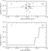 |
Fig. 2 a) C i abundance versus log τ5000(aver), average depth of line formation on the log τ5000 scale. The dashed line is the best fit straight line to the plotted points. b) Vertical abundance distribution as function of log τ5000 obtained by the trial and error applied to C ii λλ 1335.663, 1335.708 Å. |
We were able to fit, at the same time, both the core and wings of C ii at 1335.663, 1335.708 Å with the carbon abundance profile, shown in Fig. 2b, obtained with trial and error.
In Fig. 3 the C i and C ii lines computed with both the average carbon abundance −5.5 dex and the abundance step function shown in Fig. 2b are plotted. They are compared with each other and with the observed spectrum. We point out that while the step function improves the agreement between the observed and computed spectra, as shown in Fig. 3, some non-negligible inconsistencies are still present. In particular, the C ii line at 1323.9 Å is still poorly reproduced. As already discussed at the beginning of Sect. 4, we would like to stress that a NLTE analysis could clarify whether the C i anomalies are related with NLTE rather than a vertical abundance stratification.
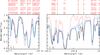 |
Fig. 3 C i lines of UV mult. 7 (λλ 1277.245, 1277.283, 1277.513, 1277.550, 1277.273, and 1277.954 Å) and the C ii blend at λλ 1335.663, 1335.708 Å computed with both the average carbon abundances of −5.5 dex (red line) and the abundance step function shown in Fig. 2b (blue line) are compared each with other and with the observed spectrum (black line). |
4.2. Nitrogen
From the absence of N i lines at 8680.282 Å and 8683.403 Å, Castelli et al. (2009) determined an upper limit of −5.82 dex ([−1.7]) for the nitrogen abundance. In the ultraviolet, the N i lines at 1411.9 Å (UV mul.10), 1310.5,1310.9 Å (UV mult. 13), and 1492.625, 1492.820, and 1494.675 Å (mult. 4) are clearly observable, as well as the lines of N ii at λλ 1275.038, 1275.251 Å and the blend at λλ 1276.201, 1276.225 Å. These lines are not all fitted by the same abundance. In fact, the nitrogen abundance is affected by both an ionization anomaly and line-to-line variations: while −5.2 dex reproduces the N ii lines, lower values, ranging from −5.9 dex to −6.8 dex, are required to fit the N i lines. The nitrogen abundance versus log τ5000(aver) is shown in Fig. 4a. A steep dependence of the abundance on the optical depth is evident. The abundance inconsistencies decrease if the abundance profile shown in Fig. 4b is used. We obtained this profile from al the N i and N ii lines with the trial and error.
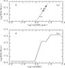 |
Fig. 4 a) Nitrogen abundance versus log τ5000(aver); crosses are for N i, circles for N ii. The dashed line is the best fit straight line to the plotted points. b) Vertical abundance distribution as a function of log τ5000 obtained by trial and error. |
The N i and N ii lines computed both with a constant abundance −5.23 dex derived from the N ii lines and with the abundance step profile shown in Fig. 4b, are compared and with the observed spectrum in Figs. 5 and 6, respectively. The effect of a depth-dependent abundance is large for the N i lines, while it does not affect the observed N ii lines.
We note that nitrogen is predominantly singly ionized in late B-star atmospheres, so that the analysis of N i could be particularly susceptible to NLTE effects in the ionization equilibrium. For N i as well as for C i a NLTE analysis is required to state the degree of reliability of the hypothesis of vertical abundance stratification for this element.
4.3. Silicon
A unique silicon abundance cannot be determined from the analysis of several silicon lines present such as Si ii, Si iii, and Si iv in the ultraviolet spectrum of HR 6000. In fact, the silicon abundance ranges from −8.35 dex to −6.0 dex. All the lines analyzed are collected in Table A.1.
A plot of the silicon abundance versus log τ5000(aver) shows a dependence of the abundance on the optical depth, with upper layers more depleted than the deeper layers (Fig. 7a).
A further significant illustration of the probable silicon stratification in HR 6000 is given by the Si ii lines at 1264.738 Å and 1265.002 Å which show a core that is consistent with an abundance of −8.35 dex and wings consistent with an abundance of −6.65 dex (Fig. 8). This Si ii line was used to derive, by means of trial and error, the empirical stratification step profile given in Fig. 7b. Its use in the spectral synthesis allows us to fit numerous Si i and Si ii lines simultaneously.
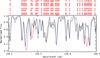 |
Fig. 5 N i lines of UV mult. 4 at λλ 1492.625, 1492.820, and 1494.675 Å computed both with the constant nitrogen abundance −5.23 dex (red line) and with the abundance step function shown in Fig. 4b (blue line). The computed spectra are superimposed to the observed spectrum. The effect of the two different adopted abundances (constant or variable) is evident. |
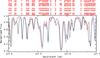 |
Fig. 6 N ii lines at λλ 1275.038, 1275.251, 1276.201, and 1276.225 Å computed both with the constant nitrogen abundance −5.23 dex (red line) and with the abundance step function shown in Fig. 4b (blue line). Only the lines at 1275.038 Å and 1276.201 Å are predicted. The computed spectra are superimposed to the observed spectrum. The effect of the two different adopted abundances (constant or variable) is negligible. |
The Alecian & Stift (2010) computations of diffusion of silicon in HgMn stars predict a stratification profile with a maximum underabundance between −0.75 dex and −2.0 dex for Teff between 14 000 K and 12 000 K, and log g = 4. It occurs at log τ5000 = −2.0. The empirical stratification profile shown in Fig. 7b implies a silicon abundance that is much lower in the whole atmosphere than that predicted by Alecian & Stift (2010).
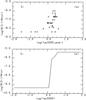 |
Fig. 7 a) Silicon abundance versus log τ5000(aver); crosses are for Si ii, circles for Si iii, triangles forSi iv. b) Vertical abundance distribution as a function of log τ5000 obtained by trial and error. |
 |
Fig. 8 Si ii lines at 1264.738 Å and 1265.002 Å computed with the average silicon abundance −7.35 dex (red line) and the abundance step function of Fig. 7b (blue line). The computed spectra are superimposed on the observed spectrum (black line). |
4.4. Phosphorous
There are numerous lines of P i, P ii, and P iii in the spectrum of HR 6000, but they are all more or less blended in the ultraviolet, except for P i at 2136.182 Å, and 2149.142 Å and P ii at 2285.105 Å and 2497.372 Å. We used NIST log gf values for most P i lines and for the P ii lines of UV multiplet 2 at 1301−1310 Å. For the remaining P i, P ii, and P iii lines we adopted log gf values from the Kurucz (2016) database. For P ii, they do not differ more than 0.01 dex from the NIST values and cover a larger number of lines than the NIST database does.
The average abundances from the P i and P ii ultraviolet lines are −5.53 ± 0.08 dex and −4.54 ± 0.11 dex, respectively, so that they differ by 1.0 dex. Because all the ultraviolet P iii lines are blended, the P iii average abundance is rather uncertain. We assumed an upper limit of log (NP iii/Ntot) ≤−5.22 ± 0.32 dex.
Castelli & Hubrig (2007) did not observe P i lines in the UVES spectrum, while several P ii and P iii unblended lines were measured. The observed cores of the strong P ii lines of multiplet 5 at λλ 6024, 6034, and 6043 Å were so deep that they could not be fitted by the computations for any abundance. In this paper, we determined two average abundances from the optical P ii lines depending on whether they lie shortward or longward of 5200 Å. These average abundances are −4.57 ± 0.1 dex and −4.32 ± 0.09 dex, respectively. The average abundance from the optical P iii lines is −4.69 ± 0.09. Table 2 summarizes all the above abundance values.
The difference of 1.0 dex, or even larger, between P i and P ii abundances and the increasing of the P ii abundance from about −4.65 dex at 4000 Å to about −4.3 dex at 6000 Å, led us to search for the presence of vertical abundance stratification for phosphorous.
In Fig. 9, the P i, P ii, and P iii abundances derived from both ultraviolet and optical lines listed in Table A.1 are plotted as a function of log (τ5000)(aver). While there is a weak dependence on depth for P ii (circles), no dependence is present for P i (crosses), which seems to have been formed at the same layers as P ii and P iii, in spite of the abundance difference of 1 dex. We may speculate that a NLTE analysis of P i would explain the large departure from the ionization equilibrium observed for phosphorous.
 |
Fig. 9 Phosphorous abundance versus log τ5000(aver); crosses are for P i, circles for P ii, triangles for P iii. |
4.5. Manganese
The spectrum of HR 6000 is very rich with Mn ii and Mn iii lines. The manganese abundance of −5.3 dex was obtained from the three Mn ii lines at λλ 2576, 2593, and 2605 Å, which were also adopted by Smith & Dworetsky (1993) in their abundances analysis of HgMn stars from IUE spectra. For HR 6000, we find the same abundance as Smith & Dworetsky (1993).
Although the average abundance −5.29 ± 0.21 dex reproduces almost all the lines examined, there are a few strong Mn ii lines with a computed core that is less deep than the observed core. They are indicated with the note “core” in the last column of Table A.1. Most Mn ii lines are affected by hyperfine structure. When hyperfine structure was taken into account in the computations a note “hfs” was added in the last column of Table A.1. To compute the hyperfine components we used the hyperfine constants measured by Holt et al. (1999) and by Townley-Smith et al. (2016).
In order to find a good sample of Mn iii lines, we examined the lines with log gf values computed by Uylings & Raassen (1997) and extracted the isolated lines and the main components of blends from them (Table A.1). The difference between the log gf values from Uylings & Raassen (1997) and those computed by Kurucz (2016) are on the order of 0.05 dex, except for two lines at 1283.589 Å and 1287.584 Å for which the difference is 0.13 dex. The Mn iii abundance equal to −5.79 ± 0.36 dex was derived using the Kurucz log gf values. Their general agreement with those from Uylings & Raassen (1997) supports the finding of 0.5 dex lower Mn iii abundance compared to the Mn ii value.
Figure 10a shows the Mn ii and Mn iii abundances versus log τ5000(aver). A dependence of the Mn iii abundance (circles) on the optical depth is manifest, while the Mn ii abundance (crosses) is constant with depth. However, the abundance adopted for the strong lines did not fit the line center. An increase of abundance or microturbulent velocity increases the wings rather than the line core.
 |
Fig. 10 a) Manganese abundance versus log τ5000(aver); crosses are for Mn ii, circles for Mn iii. b) Vertical abundance distribution as a function of log τ5000 obtained by trial and error. The theoretical vertical stratification for Teff = 14 000 K, log g = 4.0 from Alecian & Stift (2010) is overplotted (full continous line). The dashed line is the same curve shifted by −2.25 dex in the abundance. |
 |
Fig. 11 Mn ii line at 2933.054 Å computed with the average manganese abundance −5.29 dex (red line) and the abundance step function of Fig. 10b (blue line). The computed spectra are superimposed on the observed spectrum (black line). The core of the line is well fitted by the abundance step function. The hyperfine structure is considered in the computations. |
The Alecian & Stift (2010) computations of the diffusion in HgMn stars predict for manganese a stratification profile with a behavior similar to that we derived for HR 6000, but for an overabundance about 2.5 dex larger. Figure 10b compares the vertical abundance distribution as a function of log τ5000 obtained by trial and error with that from Alecian & Stift (2010), both in the original form and shifted by −2.5 dex in abundance.
Figure 11 is an example of the better agreement between the observed and computed core achieved for a strong Mn ii line when the abundance step function is used in the computations.
4.6. Gold
There is a discrepancy of 1.0 dex between the gold abundance derived from the Au ii and Au iii lines.
Several Au ii lines can be observed in the spectrum of HR 6000, but only few of them are unblended, in particular the Au ii lines at 1740.475, 1800.579, 2000.792, and 2082.074 Å. The abundance from the line at 1800 Å is so high compared to that derived from the other lines that we suspect it is blended with some other unknown component. If we exclude this line, the average abundance from the three unblended lines of Au ii is −7.57 ± 0.09 dex. However, the other blended lines are better reproduced by a lower value equal to −8.2 dex. This value also nicely fits the weak unblended line observed at 4052.790 Å in the UVES spectrum. Several Au iii lines, mostly blended, are predicted for −8.2 dex, but they are all stronger than the observed lines. The abundance from the Au iii lines ranges from −8.5 dex to an upper limit of −10 dex.
We conclude that gold is probably affected by the abundance stratification observed for some other elements as well. Figure 12a shows the Au ii and Au iii abundances versus log τ5000(aver). The figure shows a dependence of the abundance on the optical depth, with deeper layers more depleted than the upper layers, as for manganese. Figure 12b shows the empirical abundance stratification that we derived from Au ii and Au iii lines with trial and error. The abundance stratification reduces the gold abundance inhomogeneities observed in the spectrum.
 |
Fig. 12 a) Gold abundance versus log τ5000(aver); crosses are for Au ii, circles for Au iii. b) Vertical abundance distribution as a function of log τ5000 obtained by trial and error. |
5. Conclusions
This paper has extended to the ultraviolet the abundance analysis of HR 6000 performed by Castelli & Hubrig (2007) and Castelli et al. (2009) on high-resolution spectra in the optical region. In this way we obtained a panoramic view of the spectrum and abundances of all the species observed in this highly anomalous, ultrasharp-lined, non-magnetic, main-sequence, chemically peculiar star.
Thanks to ultraviolet analysis we increased the number of the elements for which abundances can be assigned, because some elements are only observable in the ultraviolet. Also some other elements, which were observed in only one ionization degree in the optical region, are present in more ionization degrees in the ultraviolet. In particular, ions not observed in the visible are: B ii, N i, N ii, Al ii, Al iii, Si iii, Si iv, P i, Sc iii, Ti iii, V ii, Cr iii, Mn iii, Fe iii, Ni iii, Cu ii, Zn ii, Ga ii, Ga iii, Ge ii, As ii, Y iii, Zr iii, Cd ii, In ii, Sn ii, Xe i, and Au iii.
The comparison of the average abundances of HR 6000 with those of other HgMn stars taken from the Ghazaryan & Alecian (2016) compilation has pointed out the strong underabundance of silicon, already found in other studies, followed by the underabundances determined from Co ii, Cu ii, Sr ii, and Zr iii. These elements put HR 6000 outside of the group of HgMn stars according to the abundances collected by Ghazaryan & Alecian (2016). At the lower underabundance limit of the Ghazaryan & Alecian (2016) compilation there is carbon, while phosphorous and iron are at the upper overabundance limit.
We found in this paper that the striking silicon underabundance ([−2.80 ± 0.26]) is not constant with depth, but that vertical abundance stratification accounts for most of the abundance anomalies observed for this element in the ultraviolet. It was modeled with an empirical step function with abundances ranging from −5.35 dex at the bottom of the atmosphere to −9.35 dex at the top of the atmosphere. We examined the possibility of abundance stratification also for some other elements which either do not meet the ionization balance requirement, such as nitrogen, phosphorous, manganese, and gold, or show strong broad profiles that cannot be fitted by an unique abundance, such as C ii at λλ 1335.663, 1335.708 Å. For all these elements, except for carbon and phosphorous, we found both a dependence of the abundance on the optical depth and an empirical abundance profile, which reduces the disagreement between the observed and computed spectra when it is adopted in the synthetic spectrum computation. For carbon, we found an empirical stratified abundance profile which roughly fits both the core and wings of C ii at λλ 1335.663, 1335.708 Å, reduces the disagreement between a few observed and computed C i profiles, but still does not explain other discrepancies, in particular that for C ii at 1323.9 Å. For phosphorous, we pointed out a weak dependence of the P ii abundance on the optical depth, but the presence at the same depths of P i and P ii lines with abundances differing by 1 dex, has hampered any determination of some empirical abundance stratification profile.
Other elements could be affected by abundance stratification, such as, for instance, yttrium and gallium, which were not analyzed here because there were too few observed lines or their log gf values were uncertain. There are other elements that do not show any sign of vertical stratification. This is true for iron in spite of its high overabundance.
In this paper we estimated abundance stratification profiles for C , N , Si , Mn , and Au in an empirical way by using the trial and error method. We are aware that a more rigorous approach should be used, taking into account either an empirical abundance stratification on the temperature-pressure structure of the model atmosphere (Nesvacil et al. 2013) or including the diffusion velocities in the model atmosphere computations (Alecian & Stift 2010; Stift & Alecian 2012). Last but not least, NLTE effects on the HR 6000 abundances should be investigated. We note that while numerous NLTE analyses were performed for stars hotter than 15 000 K and stars cooler than 10 000 K, very few and sparse work on NLTE has been carried out in the temperature range covered by the HgMn stars and, in particular, for the ultraviolet region.
Acknowledgments
We thank grant GO-13346, from the Space Telescope Science Institute, for providing support for the ASTRAL Large Treasury Project.
References
- Alecian, G., & Artru, M. C. 1988, in The Impact of Very High S/N Spectroscopy on Stellar Physics, IAU Symp., 132, 235 [NASA ADS] [Google Scholar]
- Alecian, G., & Stift, M. J. 2010, A&A, 516, A53 [NASA ADS] [CrossRef] [EDP Sciences] [Google Scholar]
- Alonso-Medina, A., Colón, C., & Rivero, C. 2005, Phys. Scr., 71, 154 [NASA ADS] [CrossRef] [Google Scholar]
- Andersen, J., & Jaschek, M. 1984, A&AS, 55, 469 [NASA ADS] [Google Scholar]
- Andersen, J., Jaschek, M., & Cowley, C. R. 1984, A&A, 132, 354 [NASA ADS] [Google Scholar]
- Ansbacher, W., Pinnington, E. H., Kernahan, J. A., & Gosselin, R. N. 1986, Can. J. Phys., 64, 1365 [NASA ADS] [CrossRef] [Google Scholar]
- Asplund, M., Grevesse, N., Sauval, A. J., & Scott, P. 2009, ARA&A, 47, 481 [NASA ADS] [CrossRef] [Google Scholar]
- Ayres, T. R. 2010, ApJS, 187, 149 [NASA ADS] [CrossRef] [Google Scholar]
- Ayres, T. R., et al. 2014, AAS Meeting Abstracts #223, 254.37 [Google Scholar]
- Babel, J. 1994, Pulsation; Rotation; and Mass Loss in Early-Type Stars, 162, 333 [NASA ADS] [CrossRef] [Google Scholar]
- Bailey, J. D., & Landstreet, J. D. 2013, A&A, 551, A30 [NASA ADS] [CrossRef] [EDP Sciences] [Google Scholar]
- Bessell, M. S., & Eggen, O. J. 1972, ApJ, 177, 209 [NASA ADS] [CrossRef] [Google Scholar]
- Biemont, E., Morton, D. C., & Quinet, P. 1998, MNRAS, 297, 713 [NASA ADS] [CrossRef] [Google Scholar]
- Biémont, É., Blagoev, K., Fivet, V., et al. 2007, MNRAS, 380, 1581 [NASA ADS] [CrossRef] [Google Scholar]
- Biémont, É., Blagoev, K., Engström, L., et al. 2011, MNRAS, 414, 3350 [NASA ADS] [CrossRef] [Google Scholar]
- Castelli, F. 2005, Mem. Soc. Astron. It. Suppl., 8, 44 [Google Scholar]
- Castelli, F., & Hubrig, S. 2007, A&A, 475, 1041 [NASA ADS] [CrossRef] [EDP Sciences] [Google Scholar]
- Castelli, F., & Kurucz, R. L. 2010, A&A, 520, A57 [NASA ADS] [CrossRef] [EDP Sciences] [Google Scholar]
- Castelli, F., Cornachin, M., & Hack, M. 1981, Liege Int. Astrophys. Colloq., 23, 149 [NASA ADS] [Google Scholar]
- Castelli, F., Cornachin, M., Morossi, C., & Hack, M. 1985, A&AS, 59, 1 [NASA ADS] [Google Scholar]
- Castelli, F., Kurucz, R., & Hubrig, S. 2009, A&A, 508, 401 [NASA ADS] [CrossRef] [EDP Sciences] [Google Scholar]
- Castelli, F., Kurucz, R. L., & Cowley, C. R. 2015, A&A, 580, A10 [NASA ADS] [CrossRef] [EDP Sciences] [Google Scholar]
- Catanzaro, G., Leone, F., & Dall, T. H. 2004, A&A, 425, 641 [NASA ADS] [CrossRef] [EDP Sciences] [Google Scholar]
- Catanzaro, G., Giarrusso, M., Leone, F., et al. 2016, MNRAS, 460, 1999 [NASA ADS] [CrossRef] [Google Scholar]
- Cugier, H., & Hardorp, J. 1988, A&A, 197, 163 [NASA ADS] [Google Scholar]
- Curtis, L. J., Matulioniene, R., Ellis, D. G., & Fischer, C. F. 2000, Phys. Rev. A, 62, 052513 [NASA ADS] [CrossRef] [Google Scholar]
- Dunlop, J. 1829, MmRAS, 3, 257 [NASA ADS] [Google Scholar]
- Eggen, O. J. 1975, PASP, 87, 37 [NASA ADS] [CrossRef] [Google Scholar]
- Enzonga Yoca, S., Biémont, É., Delahaye, F., Quinet, P., & Zeippen, C. J. 2008, Phys. Scr., 78, 025303 [NASA ADS] [CrossRef] [Google Scholar]
- Fivet, V., Quinet, P., Biémont, É., & Xu, H. L. 2006, J. Phys. B At. Mol. Phys., 39, 3587 [NASA ADS] [CrossRef] [Google Scholar]
- Fuhr, J. R., & Wiese, W. L. 1998, in CRC Handbook of Chemistry and Physics, ed. D. R. Lide (Boca Raton: CRC Press) [Google Scholar]
- Gavrila, M. 1967, Phys. Rev., 163, 147 [NASA ADS] [CrossRef] [Google Scholar]
- Ghazaryan, S., & Alecian, G. 2016, MNRAS, 460, 1912 [NASA ADS] [CrossRef] [Google Scholar]
- Grevesse, N., Scott, P., Asplund, M., & Sauval, A. J. 2015, A&A, 573, A27 [NASA ADS] [CrossRef] [EDP Sciences] [Google Scholar]
- Haris, K., Kramida, A., & Tauheed, A. 2014, Phys. Scr., 89, 115403 [NASA ADS] [CrossRef] [Google Scholar]
- Hempel, M., & Holweger, H. 2003, A&A, 408, 1065 [NASA ADS] [CrossRef] [EDP Sciences] [Google Scholar]
- Hibbert, A. 1988, Phys. Scr., 38, 37 [NASA ADS] [CrossRef] [Google Scholar]
- Holt, R. A., Scholl, T. J., & Rosner, S. D. 1999, MNRAS, 306, 107 [NASA ADS] [CrossRef] [Google Scholar]
- Hubrig, S., Castelli, F., & Mathys, G. 1999, A&A, 341, 190 [NASA ADS] [Google Scholar]
- James, D. J., Melo, C., Santos, N. C., & Bouvier, J. 2006, A&A, 446, 971 [NASA ADS] [CrossRef] [EDP Sciences] [Google Scholar]
- Jönsson, P., & Andersson, M. 2007, J. Phys. B At. Mol. Phys., 40, 2417 [NASA ADS] [CrossRef] [Google Scholar]
- Khalack, V. R., Leblanc, F., Bohlender, D., Wade, G. A., & Behr, B. B. 2007, A&A, 466, 667 [NASA ADS] [CrossRef] [EDP Sciences] [Google Scholar]
- Khalack, V. R., Leblanc, F., Behr, B. B., Wade, G. A., & Bohlender, D. 2008, A&A, 477, 641 [NASA ADS] [CrossRef] [EDP Sciences] [Google Scholar]
- Kramida, A., Ralchenko, Yu., Reader, J., & NIST ADS Team 2015, NIST Atomic Spectra Database (version 5.3), National Institute of Standards and Technology, Gaithersburg, MD [Google Scholar]
- Kurtz, D. W., & Marang, F. 1995, MNRAS, 276, 191 [NASA ADS] [Google Scholar]
- Kurucz, R. L. 1970, SAO Special Report, 309, 309 [Google Scholar]
- Kurucz, R. L. 2005, Mem. Soc. Astron. It. Suppl., 8, 14 [Google Scholar]
- Kurucz, R. L. 2016, 21 ASOS Colloq., San Paulo [Google Scholar]
- LeBlanc, F., Khalack, V., Yameogo, B., Thibeault, C., & Gallant, I. 2015, MNRAS, 453, 3766 [NASA ADS] [CrossRef] [Google Scholar]
- Leckrone, D. S., Proffitt, C. R., Wahlgren, G. M., Johansson, S. G., & Brage, T. 1999, AJ, 117, 1454 [NASA ADS] [CrossRef] [Google Scholar]
- Leone, F. 1998, Contributions of the Astronomical Observatory Skalnate Pleso, 27, 285 [NASA ADS] [Google Scholar]
- Leone, F., & Lanzafame, A. C. 1997, A&A, 320, 893 [NASA ADS] [Google Scholar]
- Leone, F., Catalano, F. A., & Malaroda, S. 1997, A&A, 325, 1125 [NASA ADS] [Google Scholar]
- Ljung, G., Nilsson, H., Asplund, M., & Johansson, S. 2006, A&A, 456, 1181 [NASA ADS] [CrossRef] [EDP Sciences] [Google Scholar]
- Michaud, G. 1970, ApJ, 160, 641 [NASA ADS] [CrossRef] [Google Scholar]
- Morton, D. C. 2000, ApJS, 130, 403 [NASA ADS] [CrossRef] [MathSciNet] [Google Scholar]
- Nesvacil, N., Shulyak, D., Ryabchikova, T. A., et al. 2013, A&A, 552, A28 [NASA ADS] [CrossRef] [EDP Sciences] [Google Scholar]
- Nielsen, K. E., Wahlgren, G. M., Proffitt, C. R., Leckrone, D. S., & Adelman, S. J. 2005, AJ, 130, 2312 [NASA ADS] [CrossRef] [Google Scholar]
- Oliver, P., & Hibbert, A. 2010, J. Phys. B At. Mol. Phys., 43, 074013 [NASA ADS] [CrossRef] [Google Scholar]
- Peterson, R. C., & Kurucz, R. L. 2015, ApJS, 216, 1 [Google Scholar]
- Proffitt, C. R., Brage, T., Leckrone, D. S., et al. 1999, ApJ, 512, 942 [NASA ADS] [CrossRef] [Google Scholar]
- Raassen, A. J. J., & Uylings, P. H. M. 1998, A&A, 340, 300 [NASA ADS] [Google Scholar]
- Reader, J., & Acquista, N. 1997, Phys. Scr., 55, 310 [NASA ADS] [CrossRef] [Google Scholar]
- Rosberg, M., & Wyart, J.-F. 1997, Phys. Scr., 55, 690 [NASA ADS] [CrossRef] [Google Scholar]
- Ryabchikova, T. A., & Smirnov, Y. M. 1994, Astron. Rep., 38, 70 [NASA ADS] [Google Scholar]
- Ryabchikova, T., Wade, G. A., & LeBlanc, F. 2003, in Modelling of Stellar Atmospheres, IAU Symp., 210, 301 [NASA ADS] [Google Scholar]
- Sansonetti, C. J., & Reader, J. 2001, Phys. Scr., 63, 219 [NASA ADS] [CrossRef] [Google Scholar]
- Scott, P., Grevesse, N., Asplund, M., et al. 2015a, A&A, 573, A25 [NASA ADS] [CrossRef] [EDP Sciences] [Google Scholar]
- Scott, P., Asplund, M., Grevesse, N., Bergemann, M., & Sauval, A. J. 2015b, A&A, 573, A26 [NASA ADS] [CrossRef] [EDP Sciences] [Google Scholar]
- Shirai, T., Reader, J., Kramida, A. E., & Sugar, J. 2007, J. Phys. Chem. Ref. Data, 36, 509 [NASA ADS] [CrossRef] [Google Scholar]
- Sigut, T. A. A. 2001, ApJ, 546, L115 [NASA ADS] [CrossRef] [MathSciNet] [Google Scholar]
- Smith, K. C. 1993, A&A, 276, 393 [NASA ADS] [Google Scholar]
- Smith, K. C. 1994, A&A, 291, 521 [NASA ADS] [Google Scholar]
- Smith, K. C. 1997, A&A, 319, 928 [NASA ADS] [Google Scholar]
- Smith, K. C., & Dworetsky, M. M. 1993, A&A, 274, 335 [NASA ADS] [Google Scholar]
- Stift, M. J., & Alecian, G. 2012, MNRAS, 425, 2715 [NASA ADS] [CrossRef] [Google Scholar]
- Thiam, M., LeBlanc, F., Khalack, V., & Wade, G. A. 2010, MNRAS, 405, 1384 [NASA ADS] [Google Scholar]
- Townley-Smith, K., Nave, G., Pickering, J. C., & Blackwell-Whitehead, R. J. 2016, MNRAS, 461, 73 [NASA ADS] [CrossRef] [Google Scholar]
- Uylings, P. H. M., & Raassen, A. J. J. 1997, A&AS, 125, 539 [NASA ADS] [CrossRef] [EDP Sciences] [Google Scholar]
- van den Ancker, M. E., de Winter, D., & The, P. S. 1996, A&A, 313, 517 [NASA ADS] [Google Scholar]
- Wiese, W. L., & Martin, G. A. 1980, Wavelengths and transition probabilities for atoms and atomic ions: Part 2. Transition probabilities, NSRDS-NBS, 68 [Google Scholar]
- Wyart, J.-F., Joshi, Y. N., Tchang-Brillet, L., & Raassen, A. J. J. 1996, Phys. Scr., 53, 174 [NASA ADS] [CrossRef] [Google Scholar]
- Yüce, K., Castelli, F., & Hubrig, S. 2011, A&A, 528, A37 [NASA ADS] [CrossRef] [EDP Sciences] [Google Scholar]
Appendix A: Element-by-element description of the ultraviolet spectrum of HR 6000
A short description of the elements observed in the ultraviolet spectrum of HR 6000 but not considered in the main paper is given in this Appendix.
Boron (B) Z = 5: we derived the underabundance [−0.75] from the B ii resonance line at 1362.463 Å. It is the main component of a blend with Fe ii 1362.451 Å.
Carbon (C) Z = 6: see the main paper.
Nitrogen (N) Z = 7: see the main paper.
Oxygen (O) Z = 8: only the three lines of the O i UV multipet 2 at λλ 1302.2, 1304.8, and 1306.0 Å can be observed in the spectrum. The abundance −3.68 dex derived by Castelli et al. (2009) from the optical region fits the lines at 1304.858 Å and 1306.020 Å. The resonance line at 1302.168 Å is blended with a strong interstellar or circumstellar component that is blueshifted by about 0.05 Å, so that only the red part of the profile is closely predicted. Although oxygen is marginally underabundant ([−0.3]), there are only two stars in the Ghazaryan & Alecian (2016) sample with even lower oxygen abundance ([−0.4]).
Magnesium (Mg) Z = 12: Castelli et al. (2009) obtained the abundance of −5.66 dex from Mg ii at 4481 Å.
The Mg ii abundance from the ultraviolet is, on average, 0.25 dex larger, in that it ranges from −5.36 dex to −5.46 dex depending on the lines considered. We used the Mg ii lines at 2928.633 Å and 2936.510 Å (mult. 2), those at 2790.777 Å and 2797.998 Å (mult. 3), and the lines at λλ 1734.852, 1737.628, and 1753.474 Å. The lines of UV multiplet 1 at 2795.528 Å and 2802.705 Å cannot be used for abundance purposes because they both are contaminated by a very strong interstellar or circumstellar component. Averaging all the abundances from the visual and ultraviolet regions we obtain −5.45 ± 0.09 dex, i.e., an underabundance of [−1.0] that is fully compatible with that of the other HgMn stars of the Ghazaryan & Alecian (2016) sample.
The observed Mg i resonance line at 2852.126 Å is very sharp and much stronger than that computed for −5.36 dex,which is the largest abundance derived from the Mg ii lines. It is probably blended with a strong line of interstellar or cicumstellar origin.
Aluminium (Al) Z = 13: Castelli et al. (2009) fixed an upper limit for the aluminium abundance of −7.30 dex from the absence of Al i and Al ii lines in the UVES spectrum. In the ultraviolet, the resonance line of Al ii at 1670.787 Å is blended with a blue interstellar (circumstellar) component, so that it cannot be used. Other lines of Al ii are well reproduced by the average abundance of −7.80 ± 0.3 dex. Al iii lines at 1854.716 Å and 1862.790 Å are better fitted by the 0.1 dex higher abundance of −7.70 dex. No lines of Al i were clearly detectable. We note that all the lines considered are more or less blended, except perhaps for Al ii at 1862.311 Å.
The average abundance from all the Al ii and Al iii lines listed in Table A.1 is −7.80 ± 0.3 dex, corresponding to an underabundance of [−2.19]. This value is compatible with the underabundances of the HgMn stars of the Ghazaryan & Alecian (2016) sample.
Silicon (Si) Z = 14: see the main paper.
Phosphorus (P) Z = 15: see the main paper
Sulfur (S) Z = 16: a sulfur abundance of −6.26 dex was obtained by Castelli et al. (2009) from the weak unblended S ii line at 4162.665 Å. Using the sulfur ultraviolet lines we updated the abundance to −6.36 dex, a value that agrees well with both the ultraviolet S i unblended line at 1425.03 Å and the S ii line of UV mult. 1 at 1250.584 Å. The other two lines of S ii mult. 1 at 1253.811 Å and 1259.519 Å are too blended with other strong lines, and probably also with some interstellar or circumstellar component, to be used for abundance purposes. All the three strong S ii lines of UV mult. 1 lie in a spectral region affected by several uncertainties mostly related with the continuum position and numerous unidentified lines. The sulfur underabundance of [−1.44] puts HR 6000 among the HgMn stars with a very low sulfur abundance according to the Ghazaryan & Alecian (2016) compilation.
Chlorine (Cl) Z = 17: the ground-state line of Cl i at 1379.528 Å is absent in the STIS spectrum. For this reason, we adopted as chlorine abundance the upper limit −7.74 dex ([−1.20]) inferred by Castelli et al. (2009) from the absence in the UVES spectrum of the line at 4794.556 Å. Other Cl i lines, if present in the UVES spectrum, are heavy blended with stronger components. Only two stars in the Ghazaryan & Alecian (2016) sample have chlorine abundance. These are χ LupiA and HD 46866 with underabundance [−1.40] and [−0.36], respectively. The underabundance of HR 6000, which is ≤[−1.20], puts the star in between χLupiA and HD 46866.
Calcium (Ca) Z = 20: the average calcium abundance obtained from a few ultraviolet unblended lines lying in the region 2110−2210 Å is almost solar (Table A.1). The underabundance of [−0.02] ± 0.09 agrees with the calcium abundance of the HgMn stars of the Ghazaryan & Alecian (2016) sample, which is more or less scattered around the solar value.
Scandium (Sc) Z = 21: only weak lines of Sc iii were observed in the STIS spectrum. From the unblended line of Sc iii at 1603.064 Å an abundance of −10.2 dex was deduced, corresponding to the underabundance of ([−1.11]). There are four stars in the Ghazaryan & Alecian (2016) sample with a scandium underabundance less than that of HR 6000. Therefore, HR 6000 is similar to other HgMn stars as far as the scandium abundance is concerned.
Titanium (Ti) Z = 22: Castelli et al. (2009) derived a titanium abundance equal to −6.47 ± 0.13 dex ([+0.64]) from the equivalent widths of numerous Ti ii lines observed in the UVES spectrum. This value was confirmed in the ultraviolet by the analysis of several Ti ii lines, in particular those at λλ 1909.207, 1909.662, and 1910.954 Å. Several Ti iii lines of the UV multiplets 1, and 3–7 were examined. There is a large spread in the abundances, which range from −6.0 dex to −7.7 dex (Table A.1). Most lines are blended. In addition, the only source for the log gf values is the Kurucz line list so that we do not have a critical compilation of the Ti iii oscillator strengths. The average abundance of Ti ii agrees within the error limits with the average Ti iii abundance −6.37 ± 0.41 dex. According to the Ghazaryan & Alecian (2016) compilation, the titanium overabundance [+0.64] of HR 6000 is a typical value for HgMn stars.
Vanadium (V) Z = 21: the V ii lines of multiplets 1, 10, and 12 at 2900 Å are either very weak or not even observed. From three lines at λλ 2908.817, 2924.019, and 2924.641 Å, we derived the average abundance of −9.23 ± 0.12 dex. In the Ghazaryan & Alecian (2016) compilation, there are two stars, ΦPhe and HD 71066, with a vanadium underabundance that is lower than the [−1.12] value of HR 6000.
Chromium (Cr) Z = 24: the lines of Cr ii and Cr iii are very numerous in HR 6000. From analyses of the Cr ii lines at λλ 2055, 2061, 2653, 2666, 2971, and 2989 Å, which are also adopted by Smith & Dworetsky (1993), and of some other unblended lines (Table A.1), we derived an average abundance of −5.9 ± 0.2 dex. This value agrees with the value of −6.10 ± 0.09 dex obtained from the optical region by Castelli et al. (2009). The Cr iii abundance was obtained from a few unblended lines that were extracted by analyzing all the Cr iii lines listed in the NIST database for the 1250−3000 Å interval. The average abundance for Cr iii is −6.22 ± 0.25 dex. The final chromium abundance −6.10 ± 0.25 dex was obtained averaging the abundances of all the Cr ii and Cr iii lines examined in both STIS and UVES spectra. According to the Ghazaryan & Alecian (2016) compilation, the chromium overabundance [+0.3] of HR 6000 is a typical value for the HgMn stars.
Manganese (Mn) Z = 25: see the main paper.
Iron (Fe) Z = 26: pratically all the lines of Fe ii and Fe iii listed in the NIST database are present in the ultraviolet spectrum of HR 6000. A few lines of Fe i, mostly those arising from the ground level, were also identified. The iron abundance −3.65 ± 0.09 dex was carefully determined by Castelli et al. (2009) from several Fe i and Fe ii lines observed in the UVES spectrum. We checked that this value closely predicts the ultraviolet Fe ii lines used by Smith & Dworetsky (1993) in their analyses of HgMn and related stars (Table A.1). The average abundance from the ultraviolet Fe ii lines is −3.68 ± 0.05 dex. This is close to the value of −3.7 ± 0.05 dex obtained by Smith & Dworetsky (1993) for HR 6000.
We extracted a set of unblended lines from the numerous Fe iii lines observed in the ultraviolet spectrum (Table A.1). The average abundance −3.78 ± 0.14 dex agrees within the error limits with the Fe ii abundance. We finally adopted the value −3.65 ± 0.09 dex deduced by Castelli et al. (2009) from the optical spectrum for the iron abundance of HR 6000. The corresponding iron overabundance, [+0.92], is an upper limit according to the Ghazaryan & Alecian (2016) compilation.
Cobalt (Co) Z = 27: Castelli et al. (2009) estimated an upper limit −8.42 dex (underabundance [−1.3]) for the cobalt abundance from the unobserved Co ii line at 3501.708 Å and from the blended Co ii line at 4160.657 Å. In the ultraviolet we examined the lines used by Smith & Dworetsky (1993) to derive the cobalt abundance in normal late-B and HgMn stars. They are the lines at λλ 2286.159, 2307.86, 2324.321, and 2580.326 Å. We added a few lines listed in Table A.1. While the line at 2307.86 Å is well predicted by −8.42 dex, the other lines, although predicted for this abundance, are not observed. Assuming that the absorption at 2307.86 Å is due to some other unidentified element, we lowered the upper limit of the cobalt abundance to −10.12 dex (underabundance [−3.0]), which suppresses the predicted unobserved lines. Smith & Dworetsky (1993) assigned the upper limit <-9.0 ± 0.5 dex for the cobalt abundance in HR 6000. The cobalt underabundance ≤[−3.0] of HR 6000 is lower than the lower limit given in the Ghazaryan & Alecian (2016) compilation.
Nickel (Ni) Z = 28: Castelli et al. (2009) obtained the abundance −6.24 dex from the equivalent width of the Ni ii line at 4067.031 Å. Smith & Dworetsky (1993) derived the nickel abundance in the HgMn stars of their sample from the Ni ii lines at λλ 2165.550, 2184.602, 2270.212, and 2287.081 Å. For HR 6000 they determined −6.34 dex. In the STIS spectrum the above lines are well fitted by −6.24 dex. The corresponding underabundance is [−0.40]. There are several Ni iii lines in the spectrum, but they are all blended except for λλ 1774.896, 1829.986, and 1830.060 Å. The average abundance from the three lines quoted above is −6.64 ± 0.14. We adopted as nickel abundance −6.24 dex from Ni ii, mostly because Ni ii is the dominant ion. According to the Ghazaryan & Alecian (2016) compilation, the nickel underabundance [−0.40] of HR 6000 is a typical value in HgMn stars.
Copper (Cu) Z = 29: Castelli et al. (2009) derived an upper limit for the copper abundance equal to −7.83 dex (solar value) from the Cu ii unobserved lines at 4909.734 Å and 4931.698 Å. In the ultraviolet, the abundance −10.53 dex was derived from the Cu ii resonance line at 1358.773 Å. The corresponding underabundance is [−2.7]. This value is well below the lower limit of [−0.89] for 112 Her A of the Ghazaryan & Alecian (2016) compilation.
Zinc (Zn) Z = 30: the zinc abundance of −8.84 dex was derived from the very weak Zn ii line at 2064.227 Å. In fact, the two strong resonance lines at 2025.502 Å and 2062.004 Å are not useful for this purpose. They both seem to be blueshifted by 0.03 Å and the second line is computed too strong, as compared with the observed line, for −8.84 dex. We argue that the two resonance lines are blended with an interstellar or circumstellar component that affects the profiles in an unpredictable way. We assumed the abundance of −8.84 dex as an upper limit. This abundance corresponds to the underabundance ≤[−1.36], which is consistent with the zinc abundance of the HgMn stars in the Ghazaryan & Alecian (2016) sample.
Gallium (Ga) Z = 31: all the Ga ii lines are blended. The abundance −8.85 dex was derived from the Ga ii resonance line at 1414.399 Å, which is the main component in a blend. The Ga ii resonance line is compatible with that from other subordinate Ga ii lines. The resonance lines of Ga iii at 1495.045 Å and 1534.462 Å give the lower abundance −8.15 dex, so that there is a discrepancy of −0.65 dex between the Ga ii and Ga iii abundances. Because Ga ii is the dominant state, we assumed for gallium the final abundance of −8.85 dex. The overabundance [+0.17] puts HR 6000 below the lowest overabundance limit equal to [+0.81] ± 0.30 provided by 46 Aql, according to the Ghazaryan & Alecian (2016) compilation.
Germanium (Ge) Z = 32: Ge ii lines were not observed in the spectrum. The solar germanium abundance was decreased to to −9.64 dex to fit the spectrum at the position of the ground-configuration line of Ge ii at 1649.194 Å. Because the line at 1261.905 is still predicted as a strong line for this abundance, the germanium abundance was further lowered to −10.64 dex.
Arsenic (As) Z = 33: the As ii line at 1375.07 Å is predicted for a solar arsenic abundance as minor component in a blend with Ti ii which closely fits the observed spectrum. Because other As ii lines were neither observed nor predicted, we adopted the solar abundance −9.74 dex for arsenic.
Strontium (Sr) Z = 38: no Sr ii lines were observed in the whole spectrum from ultraviolet to the optical regions. We adopted the upper limit −10.07 dex derived from the absence of Sr ii at 4077.709 Å. The corresponding underabundance, ≤[−0.9], puts HR 6000 among the most deficient strontium stars of the Ghazaryan & Alecian (2016) sample.
Yttrium (Y) Z = 39: Castelli et al. (2009) obtained the abundance equal to −8.60 dex from the profiles of Y ii at λλ 3950.349, 4883.682, and 4900.120 Å. However, the strong Y iii lines at λλ 2367.228, 2414.643, 2817.023, and 2945.995 Å require the higher abundance of −7.6 dex to be fitted. Yttrium overabundance is usual among HgMn stars, with values closer to what we found from Y iii than from Y ii.
Zirconium (Zr) Z = 40: an upper limit of −10.24 dex was derived from the unobserved Zr iii line at 1941.053 Å. The corresponding underabundance ≤[−0.8] contrasts with the usual zirconium overabundance in HgMn stars, as is evident from the Ghazaryan & Alecian (2016) compilation.
Cadmium (Cd) Z = 48: the resonance line of Cd ii at 2144.393 Å, although blended, is well predicted by the abundance −7.00 dex. The almost unblended Cd ii line at 2265.018 Å and two other lines at 2312.766 and 2572.93 Å have intensities that are consistent with this abundance. However, the observed Cd ii line at 2748.549 Å is fitted by −7.4 dex. It is also redshifted by 0.007 Å, indicating that the energy levels for this line should be better determined. Cd i at 2288.728 Å is observed, but blended with several features. The most important is Fe ii 2288.022 Å. The cadmium overabundance of [+3.33] is a new finding for HR 6000 abundance analyses. In the Ghazaryan & Alecian (2016) sample only χLupi A is quoted for cadmium, which is [+0.56] overabundant in this star.
Indium (In) Z = 49: the line of In ii at 1586.331 Å is blended with two stronger Fe ii lines. The abundance −10.24 dex is not in conflict with the observed blended profile, but In iii at 1625.295 Å is predicted as a strong line that is not observed.
Tin (Sn) Z = 50: the lines of Sn ii are fitted by abundances ranging from −7.0 dex for the line at 2151.514 Å to −8.7 dex for the lines at λλ1400.440, 1474.997, and 1757.905 Å. However, there are other lines, for example, those at 1312.274 Å and 1899.881 Å which are predicted to be rather strong for −8.7 dex, but are not observed at all. We suspect that incorrect energy levels for Sn ii may be responsible. The average abundance is −8.23 ± 0.64 dex. The corresponding overabundance is[+1.77] ± 0.774 dex. The only star with Sn abundance included in the Ghazaryan & Alecian (2016) compilation is χLupi A. The Sn overabundance of this star is <[+1.38], which was derived only from the line at 2151.514 Å (Leckrone et al. 1999).
Xenon (Xe) Z = 54: the numerous Xe ii lines observed in the optical region yielded the abundance of −5.25 ± 0.17 dex (Yüce et al. 2011). There are no Xe ii lines in the ultraviolet spectrum, but two Xe i lines were observed at 1469.612 Å and 1295.588 Å. They give the abundance −5.55 ± 0.25 dex, in agreement with the Xe ii value. The xenon overabundance of HR 6000 is similar to that of most HgMn stars of the Ghazaryan & Alecian (2016) sample.
Gold (Au) Z = 79: see the main paper.
Mercury (Hg) Z = 80: Castelli et al. (2009) derived an abundance of −8.20 dex from a weak structure observed at 3983.9 Å that they interpreted as due to Hg ii affected by an isotopic anomaly. However, this abundance cannot be confirmed by the clearly observable Hg ii lines at 1649.937 Å and 1942.273 Å, which both yield the abundance of −9.6 dex, i.e., an overabundance of [+1.27]. The lower Hg ii abundance is not in conflict with the abundances from a few Hg iii lines that are predicted as minor components of blends. An example is Hg iii at 1647.471 Å.
In the Ghazaryan & Alecian (2016) compilation only 53 Tau has an overabundance of mercury that is lower than that of HR 6000.
Lines analyzed in the STIS spectrum of HR 6000.
All Tables
Adopted abundances compared with solar values, as well as with extreme (maximum and minimum) values for stars from the Ghazaryan & Alecian (2016) compilation.
All Figures
|
Fig. 1 Differences between the abundance from a selected ion of a given element in HR 6000 and the solar abundance, as they are listed in Col. 3 of Table 4. The arrow for Na, Cl, Co, Zn, Ge, Sr, and Zr indicates an upper abundance limit. The vertical full line indicates the jump from Z = 57 to Z = 77, a range in atomic numbers for which no elements were observed in HR 6000. The errors can be inferred from Col. 1 of Table 4. |
| In the text | |
|
Fig. 2 a) C i abundance versus log τ5000(aver), average depth of line formation on the log τ5000 scale. The dashed line is the best fit straight line to the plotted points. b) Vertical abundance distribution as function of log τ5000 obtained by the trial and error applied to C ii λλ 1335.663, 1335.708 Å. |
| In the text | |
|
Fig. 3 C i lines of UV mult. 7 (λλ 1277.245, 1277.283, 1277.513, 1277.550, 1277.273, and 1277.954 Å) and the C ii blend at λλ 1335.663, 1335.708 Å computed with both the average carbon abundances of −5.5 dex (red line) and the abundance step function shown in Fig. 2b (blue line) are compared each with other and with the observed spectrum (black line). |
| In the text | |
|
Fig. 4 a) Nitrogen abundance versus log τ5000(aver); crosses are for N i, circles for N ii. The dashed line is the best fit straight line to the plotted points. b) Vertical abundance distribution as a function of log τ5000 obtained by trial and error. |
| In the text | |
|
Fig. 5 N i lines of UV mult. 4 at λλ 1492.625, 1492.820, and 1494.675 Å computed both with the constant nitrogen abundance −5.23 dex (red line) and with the abundance step function shown in Fig. 4b (blue line). The computed spectra are superimposed to the observed spectrum. The effect of the two different adopted abundances (constant or variable) is evident. |
| In the text | |
|
Fig. 6 N ii lines at λλ 1275.038, 1275.251, 1276.201, and 1276.225 Å computed both with the constant nitrogen abundance −5.23 dex (red line) and with the abundance step function shown in Fig. 4b (blue line). Only the lines at 1275.038 Å and 1276.201 Å are predicted. The computed spectra are superimposed to the observed spectrum. The effect of the two different adopted abundances (constant or variable) is negligible. |
| In the text | |
|
Fig. 7 a) Silicon abundance versus log τ5000(aver); crosses are for Si ii, circles for Si iii, triangles forSi iv. b) Vertical abundance distribution as a function of log τ5000 obtained by trial and error. |
| In the text | |
|
Fig. 8 Si ii lines at 1264.738 Å and 1265.002 Å computed with the average silicon abundance −7.35 dex (red line) and the abundance step function of Fig. 7b (blue line). The computed spectra are superimposed on the observed spectrum (black line). |
| In the text | |
|
Fig. 9 Phosphorous abundance versus log τ5000(aver); crosses are for P i, circles for P ii, triangles for P iii. |
| In the text | |
|
Fig. 10 a) Manganese abundance versus log τ5000(aver); crosses are for Mn ii, circles for Mn iii. b) Vertical abundance distribution as a function of log τ5000 obtained by trial and error. The theoretical vertical stratification for Teff = 14 000 K, log g = 4.0 from Alecian & Stift (2010) is overplotted (full continous line). The dashed line is the same curve shifted by −2.25 dex in the abundance. |
| In the text | |
|
Fig. 11 Mn ii line at 2933.054 Å computed with the average manganese abundance −5.29 dex (red line) and the abundance step function of Fig. 10b (blue line). The computed spectra are superimposed on the observed spectrum (black line). The core of the line is well fitted by the abundance step function. The hyperfine structure is considered in the computations. |
| In the text | |
|
Fig. 12 a) Gold abundance versus log τ5000(aver); crosses are for Au ii, circles for Au iii. b) Vertical abundance distribution as a function of log τ5000 obtained by trial and error. |
| In the text | |
Current usage metrics show cumulative count of Article Views (full-text article views including HTML views, PDF and ePub downloads, according to the available data) and Abstracts Views on Vision4Press platform.
Data correspond to usage on the plateform after 2015. The current usage metrics is available 48-96 hours after online publication and is updated daily on week days.
Initial download of the metrics may take a while.