| Issue |
A&A
Volume 601, May 2017
|
|
|---|---|---|
| Article Number | A59 | |
| Number of page(s) | 10 | |
| Section | Galactic structure, stellar clusters and populations | |
| DOI | https://doi.org/10.1051/0004-6361/201629387 | |
| Published online | 28 April 2017 | |
Asymmetric metallicity patterns in the stellar velocity space with RAVE
1 Directorate of Science, European Space Agency (ESA-ESTEC), PO Box 299, 2200 AG Noordwijk, The Netherlands
2 Dept. FQA, Institut de Ciencies del Cosmos (ICCUB), Universitat de Barcelona (IEEC-UB), Marti Franques 1, 08028 Barcelona, Spain
e-mail: This email address is being protected from spambots. You need JavaScript enabled to view it.
3 Leibniz-Institut für Astrophysik Potsdam (AIP), An der Sternwarte 16, 14482 Potsdam, Germany
4 Université Côte d’Azur, Observatoire de la Côte d’Azur, CNRS, Laboratoire Lagrange, Bd de l’Observatoire, CS 34229, 06304 Nice Cedex 4, France
5 Kapteyn Astronomical Institute, University of Groningen, PO Box 800, 9700 AV Groningen, The Netherlands
6 Observatoire astronomique de Strasbourg, Université de Strasbourg, CNRS UMR 7550, 11 rue de l’Université, 67000 Strasbourg, France
7 The Oskar Klein Centre for Cosmoparticle Physics, Department of Physics, Stockholm University, AlbaNova, 10691 Stockholm, Sweden
8 Department of Physics and Astronomy, Johns Hopkins University, 3400 N. Charles St, Baltimore, MD 21218, USA
9 Astronomisches Rechen-Institut, Zentrum für Astronomie der Universität Heidelberg, Mönchhofstr. 12–14, 69120 Heidelberg, Germany
10 Sydney Institute for Astronomy, School of Physics A28, University of Sydney, Sydney, NSW 2006, Australia
11 E.A. Milne Centre for Astrophysics, University of Hull, Hull, HU6 7RX, UK
12 Senior CIfAR Fellow, University of Victoria, Victoria, BC V8P 5C2, Canada
13 Department of Physics, Chong Yuet Ming Physics Building, The University of Hong Kong, Pokfulam Road, Hong Kong
14 Department of Physics and Astronomy, Macquarie University, Sydney, NSW 2109, Australia
15 Western Sydney University, Locked Bag 1797, Penrith South DC, NSW 1797, Australia
16 Mullard Space Science Laboratory, University College London, Holmbury St Mary, Dorking, RH5 6NT, UK
17 Dipartimento di Fisica e Astronomia Galileo Galilei, Universita’ di Padova, Vicolo dell’Osservatorio 3, 35122 Padova, Italy
18 Faculty of Mathematics and Physics, University of Ljubljana, 1000 Ljubljana, Slovenia
Received: 24 July 2016
Accepted: 14 February 2017
Abstract
Context. The chemical abundances of stars encode information on their place and time of origin. Stars formed together in e.g. a cluster, should present chemical homogeneity. Also disk stars influenced by the effects of the bar and the spiral arms might have distinct chemical signatures depending on the type of orbit that they follow, e.g. from the inner versus outer regions of the Milky Way.
Aims. We explore the correlations between velocity and metallicity and the possible distinct chemical signatures of the velocity over-densities of the local Galactic neighbourhood.
Methods. We use the large spectroscopic survey RAVE and the Geneva Copenhagen Survey. We compare the metallicity distribution of regions in the velocity plane (vR,vφ) with that of their symmetric counterparts (−vR,vφ). We expect similar metallicity distributions if there are no tracers of a sub-population (e.g. a dispersed cluster, accreted stars), if the disk of the Galaxy is axisymmetric, and if the orbital effects of the bar and the spiral arms are weak.
Results. We find that the metallicity-velocity space of the solar neighbourhood is highly patterned. A large fraction of the velocity plane shows differences in the metallicity distribution when comparing symmetric vR regions. The typical differences in the median metallicity are of 0.05 dex with statistical significant of at least 95% confidence, and with values up to 0.6 dex. For stars with low azimuthal velocity vφ, the ones moving outwards. These include stars in the Hercules and Hyades moving groups and other velocity branch-like structures. For higher vφ, the stars moving inwards have higher metallicity than those moving outwards. We have also discovered a positive gradient in vφ with respect to metallicity at high metallicities, apart from the two known positive and negative gradients for the thick and thin disks.
Conclusions. The most likely interpretation of the metallicity asymmetry is that it is mainly due to the orbital effects of the Galactic bar and the radial metallicity gradient of the disk. We present a simulation that supports this idea.
Key words: Galaxy: kinematics and dynamics / Galaxy: structure / Galaxy: disk / Galaxy: evolution / Galaxy: abundances
ESA Research Fellow.
© ESO, 2017
1. Introduction
Galaxies evolve through a complex intermix of internal and external mechanisms. For the disk of our Galaxy, we can identify several processes that give shape to its current structure, kinematics, and to its chemical and population properties. All these processes are expected to leave kinematic imprints and a fossil record in its velocity distribution (Freeman & Bland-Hawthorn 2002). For example, the presence of a bar (a non-axisymmetric gravitational component) leaves an imprint in the velocity distribution, making it asymmetric with respect to the Galactic cylindrical coordinate vR (Dehnen 2000). In general, asymmetries in vR are a signature of breakdown of axisymmetry. This could arise either from incomplete phase mixing or from the presence of non-axisymmetric components of the potential.
Processes that play a role in sculpting the velocity distri bution are the following. Firstly, star formation takes place in gaseous complexes, forming stellar clusters that sooner or later are disrupted due to the tidal stripping and internal evolution (e.g. Spitzer 1987; Baumgardt & Makino 2003; Binney & Tremaine 2008). When these clusters dissolve they can leave imprints in the velocity space while being already quite dispersed in space (Skuljan et al. 1997). Secondly, the orbits of the stars in the disk are perturbed by the spiral arms and the bar, especially through mechanisms such as driven eccentricity and trapping at the resonances (Dehnen 2000; Kalnajs 1991; Sridhar & Touma 1996, or radial mixing, making stars migrate from the radius where they were born (e.g. Sellwood & Binney 2002; Roškar et al. 2008; Schönrich & Binney 2009; Minchev & Famaey 2010). This resonant interaction can make stars appear to be concentrated in over-densities (dynamical streams) in the velocity plane (e.g. Dehnen 2000; Antoja et al. 2009; Quillen & Minchev 2005). Satellite galaxies also perturb the orbits in the disk (e.g. Quinn et al. 1993; Kazantzidis et al. 2008; Purcell et al. 2011), which can also induce kinematic substructure (Quillen et al. 2009). Furthermore, perturbing satellites can leave stars behind in the disk that will define velocity clumps (Villalobos & Helmi 2009).
An important issue is how to distinguish between the different processes. This is necessary to ultimately decode the relative importance and roles of these mechanisms in the formation and evolution of our Galaxy. In addition to the phase-space stellar distribution of the disk, stellar ages and chemical information are key elements in this decoding. While the ages of stars are difficult to measure (e.g. Soderblom 2010; Kordopatis et al. 2016), we can use the measured chemical abundances as indicators of the time of formation of the stars and their place of origin.
Several studies have used Strömgren and high-resolution spectroscopy to find clues about the origin of some velocity over-densities. For instance, the chemical homogeneity of the stars in the group HR1614 found in Feltzing & Holmberg (2000) and De Silva et al. (2007) indicates that it is a remnant of a dispersed cluster. Other moving groups, e.g. Hyades, Sirius, Pleiades and Hercules, were at one time related to dispersed clusters. However, the large dispersions in age and metallicity of their stars (Famaey et al. 2005; Helmi et al. 2006; Antoja et al. 2008; Ramya et al. 2016) discarded this hypothesis. This favours an origin related to the resonances of the bar and the spiral arms.
In the case of resonant effects, the stellar chemistry can give clues on the type of orbit that the stars follow. For example, if there is/was a metallicity gradient in the Galaxy, as measured, e.g. in Gazzano et al. (2013), Boeche et al. (2013), Genovali et al. (2014), Hayden et al. (2014), or modelled in Minchev et al. (2013), then orbits from the inner versus outer regions of the Milky Way should have different metallicities, therefore, leaving different signatures in the combined space of chemistry and phase-space. These would potentially help us to understand which resonance causes each of the over-densities, breaking the current degeneracies (several groups can be explained by either effects of the bar or the spiral arms, Antoja et al. 2009, 2011).
Bovy & Hogg (2010) have explored this by comparing the metallicity distribution of the main known moving groups to that of the background population. They found that, in general, there are no distinguishable chemical patterns in the main over-densities, which argues in favour of an origin related to transient perturbations more than to the long lasting effect of resonances. But they also pointed out that stellar migration could have erased some of the expected metallicity signatures.
Some moving groups in the local neighbourhood seem to have an extra-galactic origin (Helmi & White 1999; Wylie-de Boer et al. 2010). Other groups remain controversial. For instance, based on chemical abundances, the Arcturus moving group was thought to be a remnant of an ancient merger event (Navarro et al. 2004) but other studies showed that its chemical and age distribution point to an internal origin (Williams et al. 2009; Bensby et al. 2014).
Here we take advantage of the large spectroscopic survey RAVE (Steinmetz et al. 2006) to explore the correlations between velocity and metallicity and the possible distinct chemical signatures of the kinematic over-densities of the local neighbourhood. We use a novel approach: we test the hypothesis that the metallicity distribution of a certain region of velocity space, e.g. in Galactic cylindrical coordinate velocities (vR,vφ), is compatible with the one for its symmetric region (−vR,vφ). This should be the case under the hypothesis of axisymmetry. But, again, this can be broken by i) incomplete phase-mixing (e.g. a sub-population that is not yet phase-mixed such as a disrupted cluster or an accreted satellite); ii) the non-axisymmetries of the potential (e.g. bar and spiral arms). In the first case, the sub-population would form a region in the velocity space with a distinct metallicity. In the second one, stars following orbits of opposite signs of vR would not have the same guiding radii, and thus, have different metallicities given by the disk metallicity gradient. This methodology has the advantage that it does not use a comparison with the background stars, which might lead to inaccurate results if the field is dominated by asymmetries and groups. We find for the first time a significant asymmetry in the metallicities for positive and negative vR.
We describe the samples in Sect. 2. In Sect. 3 we study the metallicity distribution of the velocity plane and the known moving groups. In Sect. 4 we compare the metallicity distributions of all regions in velocity space with their symmetric counterparts in vR. Finally, in Sects. 5 and 6 we study the global metallicity asymmetries and gradients seen in the velocity plane. We discuss our findings and conclude in Sect. 7.
2. Observational samples
We use the RAVE data release 5 (DR5, Kunder et al. 2017) which includes the new metallicity calibration of Kordopatis et al. (2015a). The stellar parallaxes were obtained through the Bayesian distance-finding method of Binney et al. (2014). First we select stars with i) signal-to-noise (S/N) better than 20; ii) the first morphological flag indicating that they are normal stars (Matijevič et al. 2012); and iii) converged algorithm of computation of the physical parameters (“algo_conv” flag = 0, see Kordopatis et al. 2013a). From these, we further select those in a cylinder with radius of 0.5 kpc and total height of 1 kpc centred on the Sun’s position. This results in a sample of 166 015 stars with 6D phase-space information and [M/H]. We use proper motions from UCAC4 (Zacharias et al. 2013) but we have tested that our results do not change significantly if using PPMXL (Roeser et al. 2010). The median relative distance error is 31% and the median error in vR and vφ are around 7 and 5 km s-1, respectively. The median error in metallicity [M/H] is 0.1 dex.
We also use the Geneva-Copenhagen survey (hereafter GCS, Holmberg et al. 2009) and the new metallicity re-analysis by Casagrande et al. (2011). We select stars with the flag of good quality index and with available 3D velocities and [M/H]. This sample has 11 379 stars. The median relative error in distance for this sample is 6% and the median errors in vR and vφ are 1.5 and 1.2 km s-1, respectively. This is a much more local sample, with a median distance from the Sun of 71 pc. Note that the metallicity scales of RAVE and GCS are not necessarily the same, and some small offset is expected between the measured metallicities of the two surveys (see Kordopatis et al. 2013a, their Fig. 12, for a comparison of the GCS to the RAVE metallicities).
Following Reid et al. (2014), we assume that the Sun is at X = −8.34 kpc and the circular velocity at the Sun of is v0=240 km s-1. For the velocity of the Sun with respect to the Local Standard of Rest we adopt (U⊙,V⊙,W⊙) = (10,12,7) km s-1 (Schönrich et al. 2010). The resulting value of (v0 + V⊙) /R0 is 30.2 km s-1 kpc-1, which is compatible with that from the reflex motion of the Sgr A* of 30.2 ± 0.2 km s-1 kpc-1 (Reid & Brunthaler 2004). With these values, we compute the cylindrical velocities of the stars in our samples: vR (positive towards the Galactic centre, in consonance with the usual U velocity component) and vφ (towards the direction of rotation).
3. Metallicity patterns in the local velocity plane
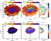 |
Fig. 1 Top: median metallicity in the velocity plane of the local neighbourhood of the RAVE sample. Left panel: 25 logarithmically spaced contours in the range spanned by the metallicity, i.e. [−0.70, 0.06]. Middle panel: same as the left one but shows contours (white) of the wavelet transform that mark the main over-densities in the velocity plane, and contours (green) that indicate significant metallicity differences (95% confidence) from its symmetric vR region. Right panel: differences in the median metallicity for positive and negative vR. The green contours are the same as for the middle panel. The numbered labels are points identified as depicting clear differences in metallicity, and whose characteristics are given in Table 1. Bottom: same for the GCS sample, with the labelled points given in Table 2. Left panel: now 25 logarithmically spaced contours in the range of [−0.34, 0.1]. |
Here we study the stellar metallicity [M/H] as a function of position in the velocity plane. We start from a grid of points in the velocity space vR−vφ separated by 2 km s-1. We assign to each point the median metallicity [M/H] of the stars in a circle of 10 km s-1. We see no differences in the results when we compute the mean metallicity instead of the median. We only consider points of the grid with at least 10 stars. We compute the error on the median metallicity through bootstrapping of 10 000 samples for each point. Since the distribution of the bootstrapped median [M/H] is not necessarily symmetric, we work with confidence limits, in particular, the 95% confidence range.
The top left panel of Fig. 1 shows the median metallicity in the velocity plane of the RAVE sample. The metallicity distribution is not uniform. The more metal rich regions are concentrated in the centre of the distribution (blue colours) while the metal poor ones are distributed in the outer parts (yellow and orange). This is likely the effect of the young stars having less velocity dispersion. We also see a highly patterned metallicity distribution: there are structures of different sizes and shapes (e.g. rounded or with branch shape) that present higher/lower metallicity than its surroundings.
To examine if there is any correlation between the metallicity patterns and the known kinematic over-densities, in the middle panel, we superpose in white the contours of the wavelet transform (WT, Starck & Murtagh 2002). The WT is a decomposition of a signal into scale-related views and thus shows over-densities of certain scales. Here we show the scale of 6 km s-1 which has been demonstrated to highlight the main known velocity over-densities (see Antoja et al. 2008, 2012, 2015b which also describe the method). The main features are:
-
an elongated feature of high metallicitiy (blue colours) thatcoincides roughly with the Hercules stream at(vR,vφ) ~ (−50,200) km s-1;
-
the region of the Hyades stream ~ (−20,240) km s-1;
-
an elongated structure, hereafter called branch 1, ranging from ~ (50,220) km s-1 to ~ (130,190) km s-1 (purple colour) that includes the Wolf 630 and Dehnen 98 moving groups (Antoja et al. 2012) and also referred to as “the horn”;
-
a velocity feature at ~ (70,250) km s-1 (hereafter branch 2), which includes part of the Sirius group, with a metallicity higher than its surroundings.
The bottom panels of Fig. 1 are for the GCS sample, where we observe a similar metallicity pattern, with also the streams of Hercules, Hyades and branch 1 being the most metal rich. Note that the colour scale used for these plots is the same but the GCS sample shows higher metallicities. This is because this sample is biased towards velocities close to the LSR and the highest metallicity part of the solar neighbourhood.
4. Metallicity asymmetries in the velocity plane
The chemical properties of the solar neighbourhood should be symmetrical in vR if there is axisymmetry. But we see in Fig. 1 that the metallicity of the velocity plane is clearly asymmetric with respect to vR = 0. Here we test the hypothesis that the metallicity distribution, and specifically its median, is the same for a point (vR1,vφ1) and its symmetric point (vR2,vφ2) = (−vR1,vφ1). To do it we compute the difference between the median metallicity of these two points:  (1)where we use the subscript 1 for the point at positive vR and 2 for the symmetric one at negative vR. This quantity is shown in the right panels of Fig. 1. The blue colours show regions where the right part of the velocity distribution (vR> 0) is more metal rich compared to the left side, and red colours show the opposite. Green lines show the velocity regions for which the statistical difference is greater than 95%. These lines are reproduced in the middle and right panels of Fig. 1.
We have chosen some representative points within these regions. In Tables 1 and 2, for the RAVE and GCS samples, respectively, we indicate for each pair of points the difference in metallicity and its significance computed as1:  (2)where σ1 and σ2 are the standard deviation of the bootstrapped medians at positive and negative vR, respectively. For RAVE (Table 1) the typical metallicity differences are around 0.1 dex. Considering all points of the grid where the differences are significant (inside the green contours), the values range from 0.009 to 0.65 with a median of 0.05 dex. For GCS, they range between 0.03 and 0.27, with a median of 0.12 dex. Note that the error on the individual stellar metallicity of RAVE is around 0.1 dex (Kordopatis et al. 2013a). However, due to the high number of stars, the median metallicity can be determined with higher precision. All cases in Table 1 have σ> 2 since we only listed points with differences of at least the 95% confidence level, and we also find points with metallicity discrepancies that are 3, 4 and up to 10σ significant.
The main velocity regions with [M/H] asymmetry are:
-
The stream of Hercules (structure at pixel IDs 3–5)with higher metallicity than the symmetric counterpart atvR> 0, with differences in [M/H] up to 0.1 dex.
-
The Hyades stream (ID 7) with slightly higher metallicity (0.04 dex) than its symmetric counterpart (approximately coinciding with branch 1).
-
The large region in the upper part of the velocity distribution (IDs 8–10) that is up to 0.17 dex more metal rich for vR> 0 compared to vR< 0. This region coincides partially with the Sirius group and branch 2.
-
Other smaller regions with higher differences in [M/H] such as those indicated with IDs 1, 2, 11 and 12. These do not correspond to any well-known kinematic over-densities.
For the GCS (Fig. 1, bottom), there are fewer regions of significant metallicity difference since there are much fewer stars in the sample. The significant regions show the same trends as for RAVE. For instance, pixel IDs GCS-3, GCS-4, GCS-6 and GCS-7 are equivalent or very close to those with RAVE IDs 4, 5, 8 and 10, respectively.
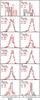 |
Fig. 2 Metallicity distributions of the locations identified in velocity space where the median metallicity is different with 95% confidence between regions with opposite vR for the RAVE sample. The panels are numbered as in the right top panel of Fig. 1. Black and red histograms are normalized and correspond to the distributions for positive and negative vR, respectively. |
Figures 2 and 3 show the metallicity distributions for the pairs of symmetric points of Tables 1 and 2, respectively. The difference in the median metallicity between the black and red distributions is evident. We see also differences in the shape of the distributions themselves (e.g. for pairs 3, 5, 6 and 11 in the RAVE sample). Note that some histograms might be affected by small number statistics, although they all led to statistically significant differences (95%) in their distributions.
5. Metallicity asymmetries as a function of velocity
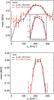 |
Fig. 4 Top: mean metallicity as a function of vφ for the positive and negative vR (black and red lines, respectively) for the RAVE sample. The error bars show the 75% confidence band. The box in the top panel shows a zoom around vφ = 200 km s-1. Bottom: same for the GCS sample. |
From Fig. 1 and Tables 1 and 2, it transpires that [M/H] 1− [M/H] 2 takes predominantly negative values for low vφ and positive values for large vφ. We analyse this trend here. We divide the velocity plane in two parts for positive and negative vR: ([− 100,0] and [0,100] km s-1) and take bins in vφ of Δvφ = 20 km s-1. Figure 4 compares the mean metallicity as a function of vφ for positive vR (black) and negative vR (red) for the RAVE (top) and GCS (bottom) samples. The error bars mark the 75% confidence limits instead of the 95% used in previous sections. We only plot bins with at least 10 stars.
The curves in Fig. 4 show a clear difference of the mean [M/H] as a function of vφ (see Sect. 6), as well as a clear difference between the metallicities for the vR< 0 stars and the vR > 0 ones. The vR < 0 stars are more metal-rich than the vR > 0 ones, except for the stars with vφ > 240 km s-1 where the contrary happens. For RAVE, the absolute differences (where they are significant) are between 0.01 and 0.5 dex, with a median of 0.03 dex. We see the same trend for the GCS, although it is not so significant. The differences are small but present at 75% confidence.
We have checked that assuming a different U⊙ does not affect significantly our results. A change in U⊙ can never smooth out completely the metallicity differences in the whole range of vφ: a U⊙ smaller than the one assumed diminishes the metallicity discrepancies for large vφ but increases them for low vφ, and the contrary when we assume a larger U⊙. Moreover, to smooth out completely one of the regimes, values up to U⊙ ~ 25 km s-1 or down to U⊙ < −5 km s-1 are necessary. We are not aware of any measurements of U⊙ of these magnitudes.
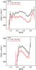 |
Fig. 5 Top: mean azimuthal velocity as a function of metallicity for positive and negative vR (black and red lines, respectively) for the RAVE sample. The error bars show the 75% confidence band. Bottom: same for the GCS sample. |
In Fig. 5 we plot vφ as a function of [M/H] for the stars in the same ranges as before (vR = [− 100,0] in red, vR = [0,100] km s-1 in black) that is the reverse of Fig. 4. We only plot bins with at least 10 stars. In this plot stars with vR > 0 have a higher mean azimuthal velocity vφ at fixed metallicity. In this case we only observe one of the regimes that we saw in Fig. 4, that is the part for high vφ. This is because the two regimes coexist for a certain metallicity, but the part for high vφ dominates because it has far more stars than the low vφ part. The difference in velocity for a fixed metallicity ranges from 4.4 to 9.4 km s-1 with a median of 7.2 km s-1 for the RAVE sample and similar values for the GCS. Note how, even though there were only two bins with significant differences in Fig. 4, now the trend appears to be very significant in Fig. 5.
6. Metallicity and azimuthal velocity gradients
In Fig. 4, independently of vR and for both samples, the metallicity increases with vφ for low vφ (< 190 km s-1), there is a flat part around vφ ~ 200 km s-1, and a decrease for vφ > 240 km s-1. This general behaviour can be linked to the known positive and negative correlations between metallicity and azimuthal velocity for the thick and thin disks, respectively. The left part of Fig. 4 (low vφ) is dominated by the thick disk, the right part (high vφ) by the thin disk, while the middle part is a mix of both components.
To measure the gradient between the rotational velocity vφ and the metallicity, we separate the samples in the two regimes where the slope is positive (vφ < 190 km s-1) and negative (vφ > 230 km s-1). Usually the inverted gradient is reported. In that case for RAVE we obtain 43.0 ± 1.0 km s-1/dex and −8.4 ± 0.2 km s-1/ dex, respectively. These values are similar to the ones in Wojno et al. (2016) who used also RAVE data to separate in a probabilistic way the two disks. The small differences might be due to a different selection of our sample (e.g. they took stars with S/N > 80 and distances < 1kpc), the fact that here we compute the gradient with unbinned data and that they took [Fe/H] instead of [M/H]. For the GCS the gradients are higher: 76 ± 6 km s-1/ dex and −18.1 km s-1/dex.
In Fig. 5, we see that the gradient in the left part of the plot (low metallicities) is not very pronounced and noisy for up to [M/H] = −0.2. This might be due to the two regimes (positive and negative gradient) coexisting in this metallicity range. For the range of [M/H] = [−0.35,0.25] dexthe data show a negative gradient of −10.1 ± 0.5 km s-1/dex. At higher metallicities ([M/H] >0.25 dex), we detect for the first time a positive gradient with slope of 18 ± 2 km s-1/dex (see Sect. 7.3 for an interpretation). The lack of stars beyond 0.5 dex in the GCS sample impede us from studying this trend in this sample but it can be perceived in the last bins.
7. Summary, discussion and conclusions
7.1. Metallicity asymmetries in the velocity plane
By studying the metallicity as a function of velocity of the solar neighbourhood in RAVE and GCS we have found that:
-
The variation of metallicity over the velocity plane is highlystructured. Most of the main velocity over-densities have adistinct metallicity compared to its velocity surroundings. This isthe case of the Hercules and Hyades streams, and of other velocitybranch-like structures.
-
A considerable part of the velocity plane shows significant metallicity differences between (vR,vφ) and its symmetric region (− vR,vφ). We obtain similar results with the two independent samples, which confirm the robustness of our findings. The typical metallicity differences are of 0.05 dex and 0.12 dex, for RAVE and GCS, respectively, with values up to 0.6 dex and at 95% confidence.
-
For low azimuthal velocity vφ, stars with negative vR (i.e. stars moving outwards in the Galaxy) have on average higher metallicity than those moving inwards. This region coincides with the Hercules and Hyades streams. On the contrary, for stars with higher vφ, the ones moving inwards (positive vR) have higher metallicity than for negative vR. The limit between the two regimes is vφ ~ 250 km s-1.
The asymmetric metallicity distribution in the velocity plane that we have found implies that there are sub-populations that are not yet well phase-mixed and/or that there is an effect of the non-axixymmetric parts of the potential.
For structures like Hercules or Hyades, we rule out the first hypothesis since it has been already shown that the metallicity, age and even mass distributions of their stars are not compatible with being remnants of a sub-population (Raboud et al. 1998; Bensby et al. 2007, 2014; de Silva et al. 2011; Pompéia et al. 2011; Famaey et al. 2007). We find a few small regions of the velocity distribution that present a distinct metallicity and do not correspond to any known velocity group, and could potentially be remnants of a cluster or a disrupted satellite. A detailed chemical analysis is required to confirm this.
Our favoured interpretation of the global asymmetries in metallicity is that they are due to the non-axisymmetries of the potential (e.g. bar and spiral arms). In this case, stars following orbits with the same vφ but opposite signs of vR would not have necessarily the same guiding radii, and thus, could have different metallicities given by the metallicity gradient of the disk (see references in Sect. 1).
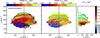 |
Fig. 6 Median orbital radius of the bins in the velocity plane of simulations in a Galactic potential with a bar. Left panel: contours every 0.25 kpc in the range of [6,10.5] kpc. Middle panel: same as the left one but shows the contours of the wavelet transform (white contours), which indicate the main over-densities in the velocity plane, and the green contours that mark the regions where the median orbital radius is significantly different with a 95% confidence from its symmetric vR region. Right panel: differences in the median orbital radius (depicted in the left and middle panels) for particles with positive and negative vR. The green contours are the same as for the middle panel. |
We use a simulation from Monari et al. (2015, 2016) to support this interpretation. The simulation consists of orbital integrations with an analytic potential for the Milky Way containing a central bar2. Figure 6 (left) shows the kinematics of stars in a solar neighbourhood-like volume colour-coded by mean orbital radius over the time when the bar is fully grown. This plot is equivalent to Fig. 1 with mean orbital radius instead of metallicity. The scale of the colour bars is such that smaller guiding radii have blue colours like higher metallicities (as would correspond to a negative radial metallicity gradient in the disk). In Fig. 6 we see a dependence on vR that makes the distribution of mean radius asymmetric with respect to the vR = 0 axis3. The differences are statistically significant: the green contours in the middle panel show the regions where the radius is different with a 95% confidence to its symmetric point in the velocity plane. This can be better seen in the right panel, where we subtract the left part of the velocity plane from the right part as we did in Fig. 1. Indeed, we obtain a very similar colour pattern compared to Fig. 1. For low vφ, the stars currently moving inwards (vR > 0) come from outer radii (ΔRmean > 0, red colours) and would have a lower metallicity compared to stars with vR < 0. For high vφ, the orbits moving inwards (vR > 0) come from inner radii (ΔRmean < 0, blue colours) and would have to a higher metallicity. This model is simple and does not include the ages of stars, but it gives a basic explanation of our findings relating them to the orbits induced by the bar of the Galaxy.
The median difference in orbital radius where there are significant differences in Fig. 6 is 0.7 kpc, with a range of [0.01,3.1] kpc. Given a metallicity gradient of −0.07 dex/kpc, this corresponds to a metallicity difference of 0.05 dex. This is similar to the median differences in RAVE, but smaller than for GCS. Note that this is only an order of magnitude estimate: the metallicity gradients in our Galaxy are very uncertain and even more their values in the past (but see Yong et al. 2012, and the models by Minchev et al. 2013). The simulation does not reproduce the small-scale metallicity structure of Fig. 1 but only the global asymmetry as function vφ. The granularity in the data could be explained by the presence of tracers of clusters, satellite remnants or other orbital effects4.
Our results caution against computing orbital eccentricities, guiding radii and other stellar orbital quantities using axisymmetric potentials. We see that in our simulation the orbits are not symmetric in vR. We observe differences of up to 3 kpc in the mean orbital radius, which is not negligible.
The metallicity asymmetry that we find in the RAVE and GCS samples is very similar to the asymmetries in the velocity plane found in Antoja et al. (2015). In that study we saw an unbalanced number of stars for positive and negative vR and also differences in the mean vR as a function of vφ. The transition point was at a very similar vφ compared to the present work and also the effects of the bar were suggested as a possible explanation. The global scenario would be the following. The bar creates an over-density of stars at vR< 0 (currently moving outwards) for low vφ that explains the existence of the Hercules stream (e.g. Dehnen 2000; Antoja et al. 2009, 2014). This stream is composed by stars following orbits that come from the inner Galaxy (thus, more metallic) compared to the stars at the same vφ but positive vR. Additionally, the bar forms an over-density of stars at vR> 0 (currently moving inwards) for high vφ that is made of stars that on average come from inner regions of the Galaxy (thus, more metallic) compared to the stars at the same vφ but negative vR.
Some studies reported azimuthal metallicity gradients in the stellar component, e.g. in clusters (Davies et al. 2009) and Cepheids (Lépine et al. 2011; Luck & Lambert 2011). These were associated to a patchy star formation driven by the bar and the incomplete mixing of metallicity in azimuth after star formation on the spiral arms, respectively. Simulations such as in Di Matteo et al. (2013), Grand et al. (2016), Miranda et al. (2016) also predict stellar azimuthal metallicity gradients due to radial migration. The connection between these gradients and the metallicity asymmetry that we find needs to be investigated.
7.2. Comparison with previous studies
Most of the previous studies found that the majority of the over-densities show large metallicity dispersion and distributions compatible with the general field population (see Sects. 1 and 7.1). Because of this, Bovy & Hogg (2010) concluded that these over-densities are more likely associated with transient perturbations. They found that the Hyades moving group is the only one with evidence for a higher metallicity than the one corresponding to its mean orbital radius in an axisymmetric model. This is consistent with an origin related to the inner Lindblad resonance of the spiral arms as suggested in Quillen & Minchev (2005). This agrees with our results where the Hyades group is more metal rich than its symmetric counterpart. Regarding the Hercules stream, Bovy & Hogg (2010) and Ramya et al. (2016) found that it shows only weak evidence of a higher metallicity than average, which would not be in agreement with being due to the bar’s outer Lindblad resonance. Liu et al. (2015) identified a structure in the age-metallicity plane, that they called narrow stripe, in the LAMOST K giant sample, which is composed by the Hercules stream and other groups. They found that this structure is made of stars with a small guiding radius (~6 kpc) but that it has an age-metallicity distribution that is consistent with stars being formed at a radius of 4 kpc. This made them conclude that these stars might have migrated from the very inner parts of the Galaxy instead of followed the resonances of the bar. However, we find that the orbits of a barred potential with median radii of ~ 6−7.5 kpc are sufficient to explain the metallicity differences of Hercules and its vR > 0 symmetric region, without any need of additional radial migration.
7.3. The azimuthal velocity-metallicity gradients
We observe a positive azimuthal velocity-metallicity gradient for low vφ and a negative one for high vφ. This is in agreement with the positive and negative gradients found for thick and thin disk, respectively (Kordopatis et al. 2011, 2013b,c, 2015b; Lee et al. 2011; Liu & van de Ven 2012b; Spagna et al. 2010; Haywood et al. 2013; Recio-Blanco et al. 2014; Wojno et al. 2016). The slopes that we measure are similar to previously reported values. The small differences could be due to the different weight of the population in each of the two regimes.
In the RAVE sample we find a new regime in the velocity-metallicity gradient: a positive gradient for high metallicity, connecting with the negative gradient of the thin disk. This is only evident when putting [M/H] on the x-axis, as the metal-rich tail only represents a small fraction of all stars at a given azimuthal velocity. Although it was not mentioned there, we see signs of the same gradient in the simulation of Loebman et al. (2011) for intermediate ages and their analysis of the GCS. This positive gradient could be a signature of radial migration mechanisms, where these metal-rich stars are migrators from the inner disk, with smaller velocity dispersions (i.e. small eccentricities) than the global population. This would naturally lead to a smaller asymmetric drift, putting them closer to the circular velocity of the Local Standard of Rest. This is consistent with the small eccentricities found for the super metal-rich stars in Kordopatis et al. (2015a, see their Figs. 6 and 9).
We have shown that the chemical measurements show asymmetries in the velocity plane which suggest the presence of incomplete phase-mixing and/or the effects of spiral arms and the bar on stellar orbits. Very soon with Gaia (Perryman et al. 2001; de Bruijne 2012) and its follow up surveys (WEAVE, 4MOST) we expect to disentangle the exact origin of each velocity over-density, to solve current model degeneracies, and to extend the study to different parts of the disk, thus building a global chemo-dynamical model of the Milky Way disk.
Note that this gives only an approximate idea of the significance of the detected signal since the bootstrapped samples may not have a symmetric distribution of median metallicities.
The bar is modelled as a quadrupole (e.g. Dehnen 2000) with a pattern speed of Ωp = 1.89Ω(R⊙), consistent with the estimate of Antoja et al. (2014). The amplitude of the bar potential is null at the beginning of the simulation, grows for 3 Gyr and is kept constant for the following 3 Gyr. The local volume is placed at an angle of −25° with the respect of the bar’s long axis, in the direction opposite to the bar’s rotation.
In an axisymmetric model, we would see a colour pattern that changes with vφ: orbits with small vφ are in their apocentres and have, thus, a smaller orbital radius, while orbits with high vφ are in their pericentres which corresponds to larger mean orbital radius.
In our model the asymmetric distribution of stars in vR is caused by the bar. However, also the spiral arms can induce strong kinematic imprints, depending on the location, pattern speed and mass of the arms (e.g. Antoja et al. 2011). We have also assumed the bar’s outer Lindblad resonance is in proximity of the Sun, as in the classical estimates of its angular velocity (e.g. Binney et al. 1997; Bissantz et al. 2003). These estimates are, however, challenged by recent models of gas dynamics and star counts in the inner Galaxy, which imply a much slower pattern speed (Wegg et al. 2015; Portail et al. 2015; Li et al. 2016).
Acknowledgments
We thank the referee, Professor Binney, for the careful reading and advice. T.A. is supported by an ESA Research Fellowship in Space Science. This work was supported by the MINECO (Spanish Ministry of Economy) – FEDER through grants ESP2016-80079-C2-1-R and ESP2014-55996-C2-1-R and MDM-2014-0369 of ICCUB (Unidad de Excelencia “Maria de Maeztu”). G.M. is supported by a postdoctoral grant from the Centre National d’Études Spatiales (CNES). A.H. acknowledges financial support from a VICI personal grant from the Netherlands Organisation for Scientific Research. We thank the CEA and Nice Observatory for the MR software. Funding for RAVE has been provided by: the Australian Astronomical Observatory; the Leibniz-Institut fuer Astrophysik Potsdam (AIP); the Australian National University; the Australian Research Council; the French National Research Agency; the German Research Foundation (SPP 1177 and SFB 881); the European Research Council (ERC-StG 240271 Galactica); the Istituto Nazionale di Astrofisica at Padova; The Johns Hopkins University; the National Science Foundation of the USA (AST-0908326); the W. M. Keck foundation; the Macquarie University; the Netherlands Research School for Astronomy; the Natural Sciences and Engineering Research Council of Canada; the Slovenian Research Agency; the Swiss National Science Foundation; the Science & Technology Facilities Council of the UK; Opticon; Strasbourg Observatory; and the Universities of Groningen, Heidelberg and Sydney. The RAVE web site is at https://www.rave-survey.org
References
- Antoja, T., Figueras, F., Fernández, D., & Torra, J. 2008, A&A, 490, 135 [NASA ADS] [CrossRef] [EDP Sciences] [Google Scholar]
- Antoja, T., Valenzuela, O., Pichardo, B., et al. 2009, ApJ, 700, L78 [NASA ADS] [CrossRef] [Google Scholar]
- Antoja, T., Figueras, F., Romero-Gómez, M., et al. 2011, MNRAS, 418, 1423 [NASA ADS] [CrossRef] [Google Scholar]
- Antoja, T., Helmi, A., Dehnen, W., et al. 2014, A&A, 563, A60 [NASA ADS] [CrossRef] [EDP Sciences] [Google Scholar]
- Antoja, T., Monari, G., Helmi, A., et al. 2015, ApJ, 800, L32 [NASA ADS] [CrossRef] [Google Scholar]
- Baumgardt, H., & Makino, J. 2003, MNRAS, 340, 227 [NASA ADS] [CrossRef] [Google Scholar]
- Bensby, T., Oey, M. S., Feltzing, S., & Gustafsson, B. 2007, ApJ, 655, L89 [NASA ADS] [CrossRef] [Google Scholar]
- Bensby, T., Feltzing, S., & Oey, M. S. 2014, A&A, 562, A71 [NASA ADS] [CrossRef] [EDP Sciences] [Google Scholar]
- Binney, J., & Tremaine, S. 2008, Galactic Dynamics: Second Edition (Princeton University Press) [Google Scholar]
- Binney, J., Gerhard, O., & Spergel, D. 1997, MNRAS, 288, 365 [NASA ADS] [CrossRef] [Google Scholar]
- Binney, J., Burnett, B., Kordopatis, G., et al. 2014, MNRAS, 437, 351 [NASA ADS] [CrossRef] [Google Scholar]
- Bissantz, N., Englmaier, P., & Gerhard, O. 2003, MNRAS, 340, 949 [NASA ADS] [CrossRef] [Google Scholar]
- Boeche, C., Siebert, A., Piffl, T., et al. 2013, A&A, 559, A59 [NASA ADS] [CrossRef] [EDP Sciences] [Google Scholar]
- Bovy, J., & Hogg, D. W. 2010, ApJ, 717, 617 [NASA ADS] [CrossRef] [Google Scholar]
- Casagrande, L., Schönrich, R., Asplund, M., et al. 2011, A&A, 530, A138 [NASA ADS] [CrossRef] [EDP Sciences] [Google Scholar]
- Davies, B., Origlia, L., Kudritzki, R.-P., et al. 2009, ApJ, 696, 2014 [NASA ADS] [CrossRef] [Google Scholar]
- de Bruijne, J. H. J. 2012, Ap&SS, 341, 31 [NASA ADS] [CrossRef] [Google Scholar]
- De Silva, G. M., Freeman, K. C., Bland-Hawthorn, J., Asplund, M., & Bessell, M. S. 2007, AJ, 133, 694 [NASA ADS] [CrossRef] [Google Scholar]
- de Silva, G. M., Freeman, K. C., Bland-Hawthorn, J., et al. 2011, MNRAS, 415, 563 [NASA ADS] [CrossRef] [Google Scholar]
- Dehnen, W. 2000, AJ, 119, 800 [NASA ADS] [CrossRef] [Google Scholar]
- Di Matteo, P., Haywood, M., Combes, F., Semelin, B., & Snaith, O. N. 2013, A&A, 553, A102 [NASA ADS] [CrossRef] [EDP Sciences] [Google Scholar]
- Famaey, B., Jorissen, A., Luri, X., et al. 2005, A&A, 430, 165 [NASA ADS] [CrossRef] [EDP Sciences] [Google Scholar]
- Famaey, B., Pont, F., Luri, X., et al. 2007, A&A, 461, 957 [NASA ADS] [CrossRef] [EDP Sciences] [Google Scholar]
- Feltzing, S., & Holmberg, J. 2000, A&A, 357, 153 [NASA ADS] [Google Scholar]
- Freeman, K., & Bland-Hawthorn, J. 2002, ARA&A, 40, 487 [NASA ADS] [CrossRef] [Google Scholar]
- Gazzano, J.-C., Kordopatis, G., Deleuil, M., et al. 2013, A&A, 550, A125 [NASA ADS] [CrossRef] [EDP Sciences] [Google Scholar]
- Genovali, K., Lemasle, B., Bono, G., et al. 2014, A&A, 566, A37 [NASA ADS] [CrossRef] [EDP Sciences] [Google Scholar]
- Grand, R. J. J., Springel, V., Kawata, D., et al. 2016, MNRAS, 460, L94 [NASA ADS] [CrossRef] [Google Scholar]
- Hayden, M. R., Holtzman, J. A., Bovy, J., et al. 2014, AJ, 147, 116 [NASA ADS] [CrossRef] [MathSciNet] [Google Scholar]
- Haywood, M., Di Matteo, P., Lehnert, M. D., Katz, D., & Gómez, A. 2013, A&A, 560, A109 [NASA ADS] [CrossRef] [EDP Sciences] [Google Scholar]
- Helmi, A., & White, S. D. M. 1999, MNRAS, 307, 495 [NASA ADS] [CrossRef] [Google Scholar]
- Helmi, A., Navarro, J. F., Nordström, B., et al. 2006, MNRAS, 365, 1309 [NASA ADS] [CrossRef] [Google Scholar]
- Holmberg, J., Nordström, B., & Andersen, J. 2009, A&A, 501, 941 [NASA ADS] [CrossRef] [EDP Sciences] [Google Scholar]
- Kalnajs, A. J. 1991, in Dynamics of Disc Galaxies, ed. B. Sundelius, 323 [Google Scholar]
- Kazantzidis, S., Bullock, J. S., Zentner, A. R., Kravtsov, A. V., & Moustakas, L. A. 2008, ApJ, 688, 254 [NASA ADS] [CrossRef] [Google Scholar]
- Kordopatis, G., Recio-Blanco, A., de Laverny, P., et al. 2011, A&A, 535, A107 [NASA ADS] [CrossRef] [EDP Sciences] [Google Scholar]
- Kordopatis, G., Gilmore, G., Steinmetz, M., et al. 2013a, AJ, 146, 134 [NASA ADS] [CrossRef] [Google Scholar]
- Kordopatis, G., Gilmore, G., Wyse, R. F. G., et al. 2013b, MNRAS, 436, 3231 [NASA ADS] [CrossRef] [Google Scholar]
- Kordopatis, G., Hill, V., Irwin, M., et al. 2013c, A&A, 555, A12 [NASA ADS] [CrossRef] [EDP Sciences] [Google Scholar]
- Kordopatis, G., Binney, J., Gilmore, G., et al. 2015a, MNRAS, 447, 3526 [NASA ADS] [CrossRef] [Google Scholar]
- Kordopatis, G., Wyse, R. F. G., Gilmore, G., et al. 2015b, A&A, 582, A122 [NASA ADS] [CrossRef] [EDP Sciences] [Google Scholar]
- Kordopatis, G., Amorisco, N. C., Evans, N. W., Gilmore, G., & Koposov, S. E. 2016, MNRAS, 457, 1299 [NASA ADS] [CrossRef] [Google Scholar]
- Kunder, A., Kordopatis, G., Steinmetz, M., et al. 2017, AJ, 153, 75 [NASA ADS] [CrossRef] [Google Scholar]
- Lee, Y. S., Beers, T. C., An, D., et al. 2011, ApJ, 738, 187 [NASA ADS] [CrossRef] [Google Scholar]
- Lépine, J. R. D., Cruz, P., Scarano, Jr., S., et al. 2011, MNRAS, 417, 698 [NASA ADS] [CrossRef] [Google Scholar]
- Li, Z., Gerhard, O., Shen, J., Portail, M., & Wegg, C. 2016, ApJ, 824, 13 [NASA ADS] [CrossRef] [Google Scholar]
- Liu, C., & van de Ven, G. 2012b, MNRAS, 425, 2144 [NASA ADS] [CrossRef] [Google Scholar]
- Liu, C., Chen, X.-Y., Yin, J., et al. 2015, ApJ, submitted [arXiv:1510.06123] [Google Scholar]
- Loebman, S. R., Roškar, R., Debattista, V. P., et al. 2011, ApJ, 737, 8 [NASA ADS] [CrossRef] [Google Scholar]
- Luck, R. E., & Lambert, D. L. 2011, AJ, 142, 136 [NASA ADS] [CrossRef] [Google Scholar]
- Matijevič, G., Zwitter, T., Bienaymé, O., et al. 2012, ApJS, 200, 14 [NASA ADS] [CrossRef] [Google Scholar]
- Minchev, I., & Famaey, B. 2010, ApJ, 722, 112 [NASA ADS] [CrossRef] [Google Scholar]
- Minchev, I., Chiappini, C., & Martig, M. 2013, A&A, 558, A9 [NASA ADS] [CrossRef] [EDP Sciences] [Google Scholar]
- Miranda, M. S., Pilkington, K., Gibson, B. K., et al. 2016, A&A, 587, A10 [NASA ADS] [CrossRef] [EDP Sciences] [Google Scholar]
- Monari, G., Famaey, B., & Siebert, A. 2015, MNRAS, 452, 747 [NASA ADS] [CrossRef] [Google Scholar]
- Monari, G., Famaey, B., Siebert, A., et al. 2016, MNRAS, 461, 3835 [NASA ADS] [CrossRef] [Google Scholar]
- Navarro, J. F., Helmi, A., & Freeman, K. C. 2004, ApJ, 601, L43 [NASA ADS] [CrossRef] [Google Scholar]
- Perryman, M. A. C., de Boer, K. S., Gilmore, G., et al. 2001, A&A, 369, 339 [NASA ADS] [CrossRef] [EDP Sciences] [Google Scholar]
- Pompéia, L., Masseron, T., Famaey, B., et al. 2011, MNRAS, 415, 1138 [NASA ADS] [CrossRef] [Google Scholar]
- Portail, M., Wegg, C., Gerhard, O., & Martinez-Valpuesta, I. 2015, MNRAS, 448, 713 [NASA ADS] [CrossRef] [Google Scholar]
- Purcell, C. W., Bullock, J. S., Tollerud, E. J., Rocha, M., & Chakrabarti, S. 2011, Nature, 477, 301 [NASA ADS] [CrossRef] [Google Scholar]
- Quillen, A. C., & Minchev, I. 2005, AJ, 130, 576 [NASA ADS] [CrossRef] [Google Scholar]
- Quillen, A. C., Minchev, I., Bland-Hawthorn, J., & Haywood, M. 2009, MNRAS, 397, 1599 [NASA ADS] [CrossRef] [Google Scholar]
- Quinn, P. J., Hernquist, L., & Fullagar, D. P. 1993, ApJ, 403, 74 [NASA ADS] [CrossRef] [Google Scholar]
- Raboud, D., Grenon, M., Martinet, L., Fux, R., & Udry, S. 1998, A&A, 335, L61 [NASA ADS] [Google Scholar]
- Ramya, P., Reddy, B. E., Lambert, D. L., & Musthafa, M. M. 2016, MNRAS, 460, 1356 [NASA ADS] [CrossRef] [Google Scholar]
- Recio-Blanco, A., de Laverny, P., Kordopatis, G., et al. 2014, A&A, 567, A5 [NASA ADS] [CrossRef] [EDP Sciences] [Google Scholar]
- Reid, M. J., & Brunthaler, A. 2004, ApJ, 616, 872 [NASA ADS] [CrossRef] [Google Scholar]
- Reid, M. J., Menten, K. M., Brunthaler, A., et al. 2014, ApJ, 783, 130 [Google Scholar]
- Roeser, S., Demleitner, M., & Schilbach, E. 2010, AJ, 139, 2440 [NASA ADS] [CrossRef] [Google Scholar]
- Roškar, R., Debattista, V. P., Quinn, T. R., Stinson, G. S., & Wadsley, J. 2008, ApJ, 684, L79 [NASA ADS] [CrossRef] [Google Scholar]
- Schönrich, R., & Binney, J. 2009, MNRAS, 396, 203 [NASA ADS] [CrossRef] [Google Scholar]
- Schönrich, R., Binney, J., & Dehnen, W. 2010, MNRAS, 403, 1829 [NASA ADS] [CrossRef] [Google Scholar]
- Sellwood, J. A., & Binney, J. J. 2002, MNRAS, 336, 785 [NASA ADS] [CrossRef] [Google Scholar]
- Skuljan, J., Cottrell, P. L., & Hearnshaw, J. B. 1997, in Hipparcos, Venice ’97, eds. R. M. Bonnet, E. Høg, P. L. Bernacca, et al., ESA SP, 402, 525 [Google Scholar]
- Soderblom, D. R. 2010, ARA&A, 48, 581 [NASA ADS] [CrossRef] [Google Scholar]
- Spagna, A., Lattanzi, M. G., Re Fiorentin, P., & Smart, R. L. 2010, A&A, 510, L4 [NASA ADS] [CrossRef] [EDP Sciences] [Google Scholar]
- Spitzer, L. 1987, Dynamical evolution of globular clusters (Princeton: Princeton University Press) [Google Scholar]
- Sridhar, S., & Touma, J. 1996, MNRAS, 279, 1263 [NASA ADS] [CrossRef] [Google Scholar]
- Starck, J.-L., & Murtagh, F. 2002, Astronomical image and data analysis (Springer) [Google Scholar]
- Steinmetz, M., Zwitter, T., Siebert, A., et al. 2006, AJ, 132, 1645 [NASA ADS] [CrossRef] [Google Scholar]
- Villalobos, Á., & Helmi, A. 2009, MNRAS, 399, 166 [NASA ADS] [CrossRef] [Google Scholar]
- Wegg, C., Gerhard, O., & Portail, M. 2015, MNRAS, 450, 4050 [NASA ADS] [CrossRef] [Google Scholar]
- Williams, M. E. K., Freeman, K. C., Helmi, A., & the RAVE Collaboration 2009, in IAU Symp. 254, eds. J. Andersen, J. Bland-Hawthorn, & B. Nordström, 139 [Google Scholar]
- Wojno, J., Kordopatis, G., Steinmetz, M., et al. 2016, MNRAS, 461, 4246 [NASA ADS] [CrossRef] [Google Scholar]
- Wylie-de Boer, E., Freeman, K., & Williams, M. 2010, AJ, 139, 636 [NASA ADS] [CrossRef] [Google Scholar]
- Yong, D., Carney, B. W., & Friel, E. D. 2012, AJ, 144, 95 [NASA ADS] [CrossRef] [Google Scholar]
- Zacharias, N., Finch, C. T., Girard, T. M., et al. 2013, AJ, 145, 44 [NASA ADS] [CrossRef] [EDP Sciences] [Google Scholar]
All Tables
All Figures
|
Fig. 1 Top: median metallicity in the velocity plane of the local neighbourhood of the RAVE sample. Left panel: 25 logarithmically spaced contours in the range spanned by the metallicity, i.e. [−0.70, 0.06]. Middle panel: same as the left one but shows contours (white) of the wavelet transform that mark the main over-densities in the velocity plane, and contours (green) that indicate significant metallicity differences (95% confidence) from its symmetric vR region. Right panel: differences in the median metallicity for positive and negative vR. The green contours are the same as for the middle panel. The numbered labels are points identified as depicting clear differences in metallicity, and whose characteristics are given in Table 1. Bottom: same for the GCS sample, with the labelled points given in Table 2. Left panel: now 25 logarithmically spaced contours in the range of [−0.34, 0.1]. |
| In the text | |
|
Fig. 2 Metallicity distributions of the locations identified in velocity space where the median metallicity is different with 95% confidence between regions with opposite vR for the RAVE sample. The panels are numbered as in the right top panel of Fig. 1. Black and red histograms are normalized and correspond to the distributions for positive and negative vR, respectively. |
| In the text | |
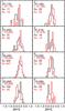 |
Fig. 3 Same as Fig. 2 but for GCS. The panels are numbered as in the right bottom panel of Fig. 1. |
| In the text | |
|
Fig. 4 Top: mean metallicity as a function of vφ for the positive and negative vR (black and red lines, respectively) for the RAVE sample. The error bars show the 75% confidence band. The box in the top panel shows a zoom around vφ = 200 km s-1. Bottom: same for the GCS sample. |
| In the text | |
|
Fig. 5 Top: mean azimuthal velocity as a function of metallicity for positive and negative vR (black and red lines, respectively) for the RAVE sample. The error bars show the 75% confidence band. Bottom: same for the GCS sample. |
| In the text | |
|
Fig. 6 Median orbital radius of the bins in the velocity plane of simulations in a Galactic potential with a bar. Left panel: contours every 0.25 kpc in the range of [6,10.5] kpc. Middle panel: same as the left one but shows the contours of the wavelet transform (white contours), which indicate the main over-densities in the velocity plane, and the green contours that mark the regions where the median orbital radius is significantly different with a 95% confidence from its symmetric vR region. Right panel: differences in the median orbital radius (depicted in the left and middle panels) for particles with positive and negative vR. The green contours are the same as for the middle panel. |
| In the text | |
Current usage metrics show cumulative count of Article Views (full-text article views including HTML views, PDF and ePub downloads, according to the available data) and Abstracts Views on Vision4Press platform.
Data correspond to usage on the plateform after 2015. The current usage metrics is available 48-96 hours after online publication and is updated daily on week days.
Initial download of the metrics may take a while.