| Issue |
A&A
Volume 601, May 2017
|
|
|---|---|---|
| Article Number | A77 | |
| Number of page(s) | 13 | |
| Section | Cosmology (including clusters of galaxies) | |
| DOI | https://doi.org/10.1051/0004-6361/201629048 | |
| Published online | 08 May 2017 | |
Ambiguities in gravitational lens models: the density field from the source position transformation
1 Argelander-Institut für Astronomie, Universität Bonn, Auf dem Hügel 71, 53121 Bonn, Germany
e-mail: This email address is being protected from spambots. You need JavaScript enabled to view it.
; This email address is being protected from spambots. You need JavaScript enabled to view it.
2 STAR Institute, Quartier Agora, Allée du six Août, 19c, University of Liège, 4000 Liège, Belgium
e-mail: This email address is being protected from spambots. You need JavaScript enabled to view it.
Received: 3 June 2016
Accepted: 24 February 2017
Abstract
Strong gravitational lensing is regarded as the most precise technique to measure the mass in the inner region of galaxies or galaxy clusters. In particular, the mass within one Einstein radius can be determined with an accuracy of the order of a few percent or better, depending on the image configuration. For other radii, however, degeneracies exist between galaxy density profiles, precluding an accurate determination of the enclosed mass. The source position transformation (SPT), which includes the well-known mass-sheet transformation (MST) as a special case, describes this degeneracy of the lensing observables in a more general way. In this paper we explore properties of an SPT, removing the MST to leading order, that is we consider degeneracies which have not been described before. The deflection field  resulting from an SPT is not curl-free in general, and thus not a deflection that can be obtained from a lensing mass distribution. Starting from a variational principle, we construct lensing potentials that give rise to a deflection field
  , which differs from
  by less than an observationally motivated upper limit. The corresponding mass distributions from these “valid” SPTs are studied: their radial profiles are modified relative to the original mass distribution in a significant and non-trivial way, and originally axi-symmetric mass distributions can obtain a finite ellipticity. These results indicate a significant effect of the SPT on quantitative analyses of lens systems. We show that the mass inside the Einstein radius of the original mass distribution is conserved by the SPT; hence, as is the case for the MST, the SPT does not affect the mass determination at the Einstein radius. Furthermore, we analyse a degeneracy between two lens models, empirically found previously, and show that this degeneracy can be interpreted as being due to an SPT. Thus, degeneracies between lensing mass distributions are not just a theoretical possibility, but do arise in actual lens modeling.
Key words: cosmological parameters / gravitational lensing: strong
© ESO, 2017
1. Introduction
Strong gravitational lensing provides a highly valuable tool to obtain mass properties of galaxies and galaxy clusters (see, e.g., Bartelmann 2010; Kochanek 2006, and references therein). In particular, multiple image systems yield strong constraints on the mass distribution. The mass enclosed within the Einstein radius presents the most robust galaxy mass estimate currently available. Furthermore, the shape of the mass distribution (e.g., ellipticity, orientation) is well defined.
However, mass estimates for radii smaller or larger than the Einstein radius are less accurate. If only a finite set of individual lensed compact images is observed, too few observational constraints are available and certainly no unique radial mass profile can be found. The situation changes somewhat if extended source components are lensed where the constraints on the mass distribution are much more stringent. Nonetheless, even if we could find a mass model which reproduces all constraints perfectly, such a mass model would not be unique either. The reason for this degeneracy is known since 1985 (Falco et al. 1985) and is called the mass-sheet transformation (MST). If a given surface mass density κ(θ) reproduces all observational constraints, then the whole family of mass models,  (1)will do the same. In particular, the MST leaves all observables invariant except the time delay1. The transformation (1) modifies the slope of the density profile with a constant factor λ. This affects mass measurements outside the Einstein radius θE and determination of the Hubble constant H0 directly.
Schneider & Sluse (2013, hereafter SS13) presented two mass profiles (namely, a Hernquist profile plus a modified Navarro, Frank and White profile, as well as a power-law mass profile) which showed almost the same imaging properties, although they are not exactly related through an MST. Following this unexpected result it became apparent that an even more general invariance transformation than the MST exists. The so-called source-position transformation (SPT) was finally introduced in Schneider & Sluse (2014, hereafter SS14).
For isolated individual images many ambiguities for the lens equation exist. Local transformations of the lensing mass distribution, which still reproduce the positional constraints from the lensed images, lead to an infinite number of mass models (see e.g., Saha & Williams 1997; Diego et al. 2005; Coe et al. 2008; Liesenborgs & De Rijcke 2012). The MST as given in Eq. (1) is a global transformation and equivalent to an isotropic uniform stretching of the source plane by a constant factor λ. The SPT is based on a more general (global) transformation of the source plane coordinates. Such transformations  , where
  denotes the transformed source position, give rise to a new deflection law
  . The new deflection law will in general not be a gradient field and thus cannot be obtained from the deflection caused by a lens. However, if the curl component of is sufficiently small, then one may find a lensing mass distribution which yields a deflection law which is very close to , so close that it cannot be observationally distinguished from . In this paper we will explore this possibility, which of course depends on the SPT
  . In particular, if this deformation is “too strong”, then the resulting cannot be approximated with the deflection due to a lens – this will restrict the freedom in choosing transformations .
The outline of the paper is as follows. In Sect. 2 we will recapitulate the principle of the SPT. We characterize the deviation of the deflection law from a gradient field quantitatively in Sect. 3 by finding a gravitational potential  such that
  is as close as possible to the SPT-transformed deflection law . To do so, we will start from a variational principle and show that the modified deflection potential has to fulfill Neumann boundary conditions. Those can be solved using a Green’s function, and the solution will be given explicitly for a circular region. Furthermore, a numerical approach will be presented to find degenerate deflection laws and their corresponding mass profiles. By considering a specific deformation function and assuming a positional accuracy on lensed image positions typical of the Hubble Space Telescope (HST), we will present in Sect. 4 the implications of the “allowed” SPTs on current mass profile determinations, regarding the radial mass profile and the angular structure of the lens. Different diagnostics for the change of the mass profile by an SPT, and how it can be distinguished from an MST, will be explored in Sect. 5 in terms of the aperture mass. Finally, we will discuss our findings in Sect. 6.
2. The principle of the source position transformation
In the following we will describe the principle of the SPT and its properties. For a more detailed account the reader is referred to SS14. We use standard gravitational lensing notation throughout this paper (see, e.g., Schneider 2006).
In general, a surface mass density distribution κ(θ) gives rise to a deflection law α(θ), where θ is the angular position in the lens plane, i.e., the observer’s sky. The mass distribution or convergence κ is defined as the ratio of projected surface mass density to the critical surface mass density, where the latter depends only on the angular diameter distances of lens and source. If that mass distribution is sufficiently concentrated (i.e., typically κ(θ) ≳ 1 for some region in the lens plane) a source may have multiple images, depending on its position relative to the deflector on the sky. Then, the source located at the (unobservable) position β will have its images at locations described by the solutions θi = β + α(θi) of the lens equation. Since multiple images are from the same source, we can deduce the constraints on the deflection law α(θ) as  (2)or likewise for an alternative deflection law
  as
as  (3)for all i<j, such that α(θ) as well as yield exactly the same sets of multiple images. If such equivalent deflection laws exist, they will correspond to source positions β = θ−α(θ) or
  , respectively (see Fig. 1).
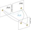 |
Fig. 1 Illustration of the source position transformation. A source at β causes multiple images θ in the lens plane under the deflection law α. The same multiple images are obtained from a source at |
We can now consider a one-to-one mapping that connects the original source coordinates to the new ones. This allows us to define the transformed deflection law as  (4)where in the last step we inserted the original lens equation β = θ−α(θ).
Hence, any bijective (i.e., one-to-one) function leads to an SPT which leaves the condition (2) invariant. Moreover, as can be deduced from the Jacobian  of the modified lens equation, the relative magnification matrices and the relative image shapes between image pairs of the same source remain unchanged. However, the Jacobian
  will not be symmetric in general, and therefore cannot be written as the gradient of a deflection potential
  (i.e., is not a curl-free field). This implies that no corresponding mass distribution
  exists that yields a deflection angle , in general. However, it was shown in SS14 that the asymmetric part of the Jacobian can be small in realistic cases; this will be explored more quantitatively in Sect. 3. In the special case that the lens is axisymmetric and the transformation corresponds to a radial stretching of the form
  (5)the SPT is an exact invariance transformation: in this case, the Jacobian is symmetric, and for every transformation (5) and its corresponding deflection law there exists a corresponding axi-symmetric mass distribution .
Provided the curl component of is small, then we expect that there exists a mass distribution  whose corresponding deflection law
  will be very similar to , in the sense that their difference is smaller than the astrometric accuracy of current observations. In this case, the SPT will be, for all practical purposes, a global invariance transformation for lenses.
3. The transformed mass distribution
3.1. The general method
Since the deflection law  (4) is not a gradient field, it does not correspond to a deflection field caused by a gravitational lens. However, if the curl component of is sufficiently small, one may be able to find a deflection potential
  and a corresponding deflection law
  such that the difference between
  is small, for example smaller than the astrometric accuracy of current observations. Since only the region of the lens plane where multiple images occur is constrained by lensing observations, the difference
  needs to be small only in a finite region, which we denote as
  .
.
We thus consider the “action”  (6)for which we want to find a minimum.
Using this particular variational principle is just one possibilty of finding . One could also apply the Helmholtz theorem and decompose into its irrotational (curl-free) and solenoidal (divergence-free) part. This would lead to similar but not identical results for , thus not changing the main conclusions of this paper2. Another possible ansatz would be to find a gradient deflection angle such that its maximum deviation from would be minimized; however, the solution of this problem seems to be much more difficult to find than our variational principle.
Equation (6) can be minimized by considering small variations of  , and finding the conditions for which the action is stationary for all variations
  . Up to linear terms in , we find
  (7)where we made use of Gauß divergence theorem. The boundary curve of is denoted as
  , ds is the line element of the boundary curve, and n(s) the outward directed normal vector. Requiring δS = 0 leads to the Neumann problem
  (8)where the first equation is required for all points
  , and the second one for all points on the boundary . The solution
  of Eq. (8) is specified only up to an additive constant, since a constant in the deflection potential does not affect the deflection angle.
In order to solve the system (8), we can either use numerical standard methods for such boundary problems, or we can obtain the solution by means of a Green’s function. Both methods will be explored in this section.
3.2. Solving the Neumann problem numerically
We defined the convergence of the transformed deflection law to be  . The curl component of is reasonably small if the closest curl-free approximation to (which is ) is smaller than a chosen astrometric accuracy εacc
 (9)for all
  . To solve the system (8) numerically, we set up a successive overrelaxation method (SOR; Press et al. 1996, their Sect. 19.5) on a square grid to calculate . An SOR is a converging iterative process based on the extrapolation of the Gauß-Seidel method, and it is a standard method to solve boundary value problems (see, e.g., Seitz & Schneider 2001). Using a second-order accurate finite differencing scheme, the deflection law is then derived from the deflection potential .
The lens is located at the center of the grid, chosen to be also the origin of the coordinate system. The grid has a length of 4 θE to cover the relevant area in which multiple images occur, i.e., it covers the region within 2θE from the lens center.
The SOR involves the calculation of a weighted average between the previous iterate  and the computed Gauß-Seidel iterate
  successively for each component
  (10)where
  is the value of for the grid point (i,k) in iteration m, and ω is the extrapolation parameter. The parameter ω is chosen such that it accelerates the rate of convergence of the iterative variable to the solution; in this work
  (11)is applied, where
  is the total number of grid points. Initially, all
  are set to zero. In each iteration m, the Gauß-Seidel iterate is calculated as follows (a fourth-order accurate finite differencing is used)
 ![Mathematical equation: \begin{eqnarray} \tilde{\Psi}_{i,k}^{(m+1)} &= &-\frac{1}{60} \, \Bigl( \ptilde_{i+2,k}^{(m)} + \ptilde_{i-2,k}^{(m)} + \ptilde_{i,k+2}^{(m)} + \ptilde_{i,k-2}^{(m)} \Bigl) \nonumber\\ &+& \frac{16}{60} \, \Bigl( \ptilde_{i+1,k}^{(m)} + \ptilde_{i-1,k}^{(m)} + \ptilde_{i,k+1}^{(m)} + \ptilde_{i,k-1}^{(m)} \Bigl) \nonumber\\ &-& \frac{12}{60} h^2 \, \bigl[ \nabla \cdot \ahat \bigl]_{i,k}, \label{eq:gaussseidel} \end{eqnarray}](/articles/aa/full_html/2017/05/aa29048-16/aa29048-16-eq70.png) (12)where h is the spacing of grid points. The divergence of is calculated with fourth-order accurate finite differencing method for each grid point, and for points on the boundary of the grid and the neighboring row and column, a second-order accurate finite differencing scheme is employed. Convergence is reached when two requirements are met: (i) at least
(12)where h is the spacing of grid points. The divergence of is calculated with fourth-order accurate finite differencing method for each grid point, and for points on the boundary of the grid and the neighboring row and column, a second-order accurate finite differencing scheme is employed. Convergence is reached when two requirements are met: (i) at least  iterations have been made; and (ii) the maximum difference
  between two iterations increases. Typically, slightly more than
  are needed to reach convergence. If the process converges, the values of at the four corners are calculated by extrapolation.
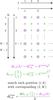 |
Fig. 2 Illustration of the extrapolation method used in the SOR method (Sect. 3.2) to calculate |

We consider that the typical accuracy on the image position of observed lens systems is of the order 5 mas, implying that εacc in Eq. (9) should be of the same order (this choice will be discussed in Sect. 4). Thus, the numerical error of our method has to be well below 1 mas ≈ 10-3θE for typical galaxy scale lenses which is quite stringent. Increasing the grid size yields a strong increase in computational time, which scales roughly as  . Therefore, we added an extrapolation method to the standard SOR to increase accuracy with a more reasonable increase in computational time. The principle of our extrapolation scheme is displayed in Fig. 2 and is based on the observation that the error | Δα | of the computed value
  scales as
  . This can be seen in the top panel of Fig. 3 where we applied our numerical scheme to the case of a non-singular isothermal sphere, i.e., where the true solution is known analytically. In this case, the deflection law is a pure gradient field, and thus
  . Using this scaling behavior we can extrapolate to the true deflection
  , which would be obtained in the limit h → 0, for every grid point
 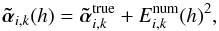 (13)where Enum is the numerical error3. However, the asymptotic deflection and the value of the numerical error Enum are unknown in general. We can determine the two unknowns by calculating for two different values of h, i.e., for different
  . Hence, we calculate on two grids, of
  and
and  points. The coordinates of the first and second grid are denoted respectively with indices (I,K) and (i,k) and we have to match every grid point (i,k) with its corresponding position (I,K). Then we can obtain the true value
 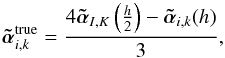 (14)as indicated in Fig. 2.
Incorporating this extrapolation method in the code decreases the numerical error for the grid point numbers that are used ( ) roughly by a factor of 103, as can be seen in the lower panel of Fig. 3, which also shows that the numerical error with this extrapolation scheme decreases much faster with
  than without. The largest numerical deviation (Δα)max can be found near the center of the grid. This is as expected, since the deviation from depends on higher-order derivatives, which for the chosen lens model are largest near the center. However, multiple images near the center of the lens are usually highly demagnified and rarely observable for galaxies as lenses (see, e.g., Hezaveh et al. 2015; Winn et al. 2004) and are therefore not relevant.
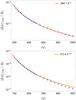 |
Fig. 3 Maximum difference of |


We have also tested the accuracy of the numerical implementation. One method is to check whether  is valid for the whole grid for any deformation function . In all our calculations, deviations
  are always smaller than 10-4 if the corner regions, i.e., θ ≥ 2 θE, are excluded from our analysis. Thus, we only consider the behavior of the mass profile in the circular region | θ | /θE< 2, where numerical errors in
  do not exceed 10-6θE.
3.3. Solution by means of a Green’s function
A different approach is to find a solution of Eq. (8) by means of a Green’s function. For that, we make use of Green’s second theorem, considering a function h(θ), 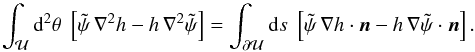 (15)We choose the function h(θ) ≡ H(ϑ;θ) depending on the vector ϑ such that it obeys the following equations:
 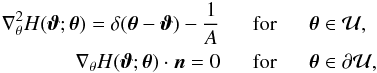 (16)where A is the area of , and ϑ is a point within . The term 1 /A in Eq. (16) is needed to satisfy Green’s divergence theorem applied to the vector field ∇h, which requires
 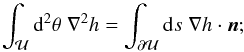 (17)the conditions (16) set both side of this equation to zero. With (16), Eq. (15) simplifies to
 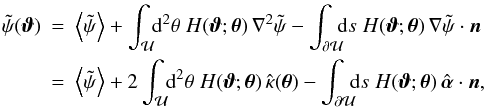 (18)where
  is the average of on
  , and we used Eq. (8) in the last step. We note that the integral
 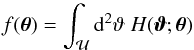 (19)is a constant, since ∇2f(θ) = 0 and n·∇f = 0 on the boundary of . Therefore, if we integrate Eq. (18) over , the two integrals on the r.h.s. compensate each other, due to the divergence theorem, so that this solution is consistent.
Whereas for a general region it will be difficult to obtain a solution of Eq. (16) for H(ϑ;θ), such a solution is analytically known if is a circle of radius R. In this case, 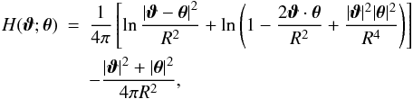 (20)which has the properties that
 Hence, Eq. (20) indeed satisfies the conditions (16).
With this explicit solution, we can now calculate the deflection angle corresponding to the potential ,  , by obtaining the gradient of H,
  (21)Then,
  (22)where we have to deal with a pole in the first term of Eq. (21). Using a conformal mapping as described in Appendix A, we can handle this pole numerically. In the third term the pole lies outside the circle and since
  there is no pole. However, if θ is on the circle (as occurs in the line integral in Eq. (22)), the third term can become quite large; hence, for points ϑ near the boundary, special care is needed to obtain an accurate solution.
This Green’s function approach has several advantages over using a SOR for a grid. First, the region on which the Neumann problem is defined can be chosen as a circle, instead of a rectangle for the SOR method. Second, the solution by means of the Green’s function yields higher accuracy. The reason for this is that the limited accuracy in finite differencing does not occur here. Third, if one is interested in the deflection only at a few points, this can be calculated much faster than with the SOR which necessarily calculated the solution over the whole region.
3.4. Interpretation
The expression (18) for the deflection potential, or the expression (22) for the deflection angle, contains quite a number of terms. In order to obtain a better understanding of the various terms, we consider again the case where the deflection angle is a pure gradient field, in which case  . Then the deflection angle at a point
  can be decomposed into a deflection αin which is caused by matter inside , and one due to matter outside , denoted by αout. Thus we expect that
  (23)Comparing the last Eqs. (23) to (22), we find that
  (24)where
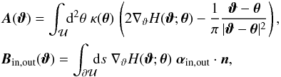 (25)where we split the deflection angle on the boundary into terms due to matter inside and outside . Both of the terms A and Bin are due to matter inside , whose deflection is covered entirely by the first term αin, so that we expect that
 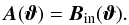 (26)In Appendix B we show explicitly that this relation holds for the case of a circular region for which H is given by Eq. (21). Hence, Eq. (24) then provides a clean separation of the deflection angle coming from the inner mass distribution (αin) and that coming from matter outside , given by Bout. This relation may be of practical relevance for the numerical calculation of the lensing properties from a complicated mass distribution, for which the lensing quantities are only needed inside a limited region. Instead of calculating, for every point inside , a two-dimensional integral of the surface mass density κ over the whole lens plane, one can proceed as follows: first, one can reduce the integration range over the region to get the contribution αin. Second, one can calculate the contribution αout for points on the boundary by integrating over the outer region of the lens in terms of a two-dimensional integral. Third, the contribution αout for points inside the region can then be obtained by a one-dimensional integration over the boundary curve.
In general, if α is given on the boundary, it contains contributions from both the inner and the outer part. In other words, the split of B into Bin and Bout is not provided in that case. The term A then compensates for the contribution Bin of B.
4. Illustrative example – a quadrupole lens and an isotropic SPT
Our goal is to find criteria allowing us to assess whether an SPT-transformed deflection law is valid (i.e. deviates from a gradient field by less than εacc), using the methods explained in the previous section. Thus, we set an upper limit on how much the transformed deflection law is allowed to differ from its closest curl-free approximation before leading to a non-negligible shift of the lensed images. Since observed lens systems are usually fit by simple mass models with only a small number of free parameters, we do not expect the fit to be perfect. We always have to deal with observational uncertainties as well as the presence of substructure (Xu et al. 2010; Bradač et al. 2004; Kochanek & Dalal 2004; Mao & Schneider 1998) and line-of-sight inhomogeneities (Xu et al. 2012; Metcalf 2005). Therefore, we cannot reproduce observed positions better than a few milliarcseconds with a smooth mass model. Hence, as long as | Δα(θ) | is less than the smallest angular scale on which modeling with a smooth mass model is still meaningful, differences are of no practical relevance (SS14).
We need to choose a lens model to explore how seriously the SPT may affect lens modeling. First, we consider a situation similar to SS14, namely a quadrupole lens with external shear γp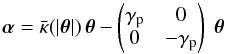 (27)which is deformed by an SPT corresponding to a radial stretching, as in Eq. (5). Specifically, we choose
 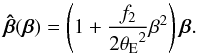 (28)This deformation function is the lowest-order expansion of more general stretching functions, and its leading-order term is chosen such as to not yield an MST, to cleanly separate the effect of the MST from that of the more general SPT in this study. Furthermore, we choose as specific lens model a non-singular isothermal sphere (NIS), described by the mean convergence profile
  (29)where θc is the core radius. For the rest of this paper, we fix the core to be θc = 0.1θE.
To get a quantitative estimate on how large deviations of  from are tolerable before the lensing properties of the SPT deviate markedly from the original lens model, we take the Hubble Space Telescope (HST) as example. We estimate that the highest astrometric accuracy that can be achieved corresponds to about a tenth of a pixel in the ACS camera, or Δθ ≈ 5 mas ≈ 5 × 10⁻³θE, where the last expression accounts for the fact that the typical Einstein radii of galaxy-scale lenses are of order one arcsecond. Thus, if the solution satisfies the condition (9) with ϵacc = 5 × 10⁻³θE over the region | θ | ≤ 2 θE, we call the corresponding SPT allowed or valid.
4.1. Impact on the deflection law
The model we consider has two free parameters, the distortion parameter f2 in the SPT (28), and the strength γp of the external shear. We start with exploring this parameter space to find the combination that yield allowed transformations, using the methods described in the previous section. In Fig. 4, we display the maximum deviation |Δα| max as a function of these two parameters. It shows a wide range of allowed parameter combinations, where the allowed range of f2 decreases with increasing external shear. The white regions in Fig. 4 denotes parameter combinations where |Δα| max > 0.005 θE, and which are therefore not allowed according to our accuracy criterion.
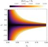 |
Fig. 4 Values of |Δα| max are plotted against the parameters f2 from (28) and external shear strength γp. The colored region indicates allowed pairs of parameters that fulfill the |Δα| < 5 × 10⁻³θE-criterion. For obtaining this figure, we used the SOR method. |
In SS14, we speculated that the curl of may yield a good indication for the deviation of the SPT-transformed deflection field from a gradient field. In this case, the curl  , which describes the asymmetric part of the Jacobian, could be used as a proxy for | Δα |. For a quadrupole lens of the form (27) and the deformation law (28), the curl
  is given in Eq. (42) of SS14,
 ![Mathematical equation: \begin{eqnarray} \ki &\approx& - \frac{\gp}{2} f_2 \left( \frac{\theta}{\tE} \right)^2 \label{eq:kiSS14}\\ &&\times \left[\gp^2 - (1 - \kbar)(2\gm + 1 - \kbar) + 2 \gm \gp \cos(2\varphi)\right] \sin 2\varphi, \nonumber \end{eqnarray}](/articles/aa/full_html/2017/05/aa29048-16/aa29048-16-eq174.png) (30)where θ,ϕ describe polar coordinates in the lens plane and
(30)where θ,ϕ describe polar coordinates in the lens plane and  is the shear caused by the NIS lens.
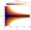 |
Fig. 5 Values of |
Figure 5 shows the maximum of  as a function of external shear γp and deformation “strength” f2, which indeed is very similar to Fig. 4. The actual difference between those two approaches is seen in Fig. 6. An approximately linear correlation with an expected but modest scatter can be seen. In fact, from that figure we obtain for our specific model that
  (31)For other models, the relation between | Δα | max and
  will be different; nevertheless, we see that the curl of indeed provides a useful indication for the validity of an SPT, since calculating is much easier then obtaining the numerical solution for .
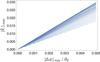 |
Fig. 6 For every allowed combination f2 and γp the values of | Δα | max (Fig. 4) are plotted against |
Figure 7 illustrates how a specific deflection law in a region | θ | ≤ 2 θE is affected by an SPT. It shows | Δα(θ) | for a quadrupole lens with external shear γp = 0.1 and deformation strength f2 = 0.55, which is the highest allowed for this value of the external shear strength and thus is expected to show the largest deviations compared to the original mass profile. The figure shows that the largest deviations occur at an angle of 45° with respect to the external shear. This pattern, which is shown for one specific pair of f2 and γp, is qualitatively the same for all f2-γp-combinations.
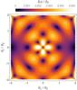 |
Fig. 7 Map of | Δα(θ) | is shown for f2 = 0.55 and γp = 0.1. The strong changes in the corners, i.e. θ > 2 θE, are biased by large numerical uncertainty and should be neglected. |
4.2. Implications for the convergence
We show in Fig. 8 the comparison between original (κ) and SPT-transformed mass distribution ( ) for three different allowed pairs of parameters, f2 = 0.55 and γp = 0.1 (the same combination of parameters as in Fig. 7), f2 = −0.55 and γp = 0.1, and f2 = 1.2 and γp = 0.05. The lower panel of Fig. 8 shows the change of the radial profile as
  .
.
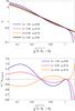 |
Fig. 8 Upper panel shows the mass profile of the original NIS lens (solid curve), and that of three SPT-transformed lenses, with parameters f2 and γp indicated by the labels. For all of these three models, Δαmax ≈ εacc = 5 × 10⁻³θE. Since the transformed mass distributions have a finite ellipticity, the density is plotted as a function of the geometric mean of the major and minor semi-axis of the best-fitting ellipse to an isodensity contour, except for the case with negative f2, for which the outer isodensity contours are not closing around the lens center; in this special case, the x-axis corresponds to the θ1-axis. The convergence changes up to 28% for radii smaller than 1 θE, radii larger than that show a significantly smaller convergence for a positive f2. Negative f2 show an essentially mirrored behavior compared to positive f2. This leads to convergence |
The divergence of (i.e.  ), was calculated analytically in SS14 (see their Eq. (41)) and can be used to compare our numerical results to the analytic solution. Specialized to our case, it reads
 ![Mathematical equation: \begin{eqnarray} \khat &= &\ \kappa_\mathrm{NIS} + \frac{f_2}{2} \left( \frac{\theta}{\tE} \right)^2 \nonumber\\\label{eq:khatSS14} && \times\biggl( \ \gamma_\mathrm{m} \Bigl[ 2 \gamma_\mathrm{p}^2 + 3 \bigl( 1 - \kbar \bigl)^2 \Bigl] \ - \ 2 \bigl( 1 - \kbar \bigl) \Bigl[ \bigl( 1 - \kbar \bigl)^2 + 2 \gamma_\mathrm{p}^2 \Bigl] \biggl. \\ && + \Bigl[ 5 \gamma_\mathrm{p} \bigl( 1 - \kbar \bigl)^2 - 6 \gamma_\mathrm{p} \gamma_\mathrm{m} \bigl( 1 - \kbar \bigl) + \gamma_\mathrm{p}^3 \Bigl] \, \cos 2 \varphi + \gamma_\mathrm{p}^2 \gamma_\mathrm{m} \, \cos 4 \varphi \biggl. \biggl). \nonumber \end{eqnarray}](/articles/aa/full_html/2017/05/aa29048-16/aa29048-16-eq200.png) (32)where again θ,ϕ describe polar coordinates in the lens plane. The change
(32)where again θ,ϕ describe polar coordinates in the lens plane. The change  is proportional to the stretching parameter f2, so that Δκ(−f2) = −Δκ(f2). This behavior can be seen in Fig. 8. Indeed, we checked that all numerically obtained deflection angles are such that their corresponding surface mass densities agree with the analytical prediction (32). For example, the numerical result for the parameter combination γp = 0.1 and f2 = 0.55 deviates by less than 3 × 10⁻³ from the analytical solution.
As seen from Eq. (32), the resulting mass distribution is no longer axi-symmetric, but that isodensity contours are nearly elliptical (i.e., a factor proportional to cos(2φ)) with a small boxiness (i.e., a factor proportional to cos(4φ)). Hence, we define the distance from the center generally as the geometric mean  using the 1- and 2-axis of the elliptical isodensity contours. However, for sufficiently negative f2, the outer isodensity contours are no longer concentric, i.e., they are not closed curves around the center of the lens. In addition, for large negative values of f2, the radial profile can become non-monotonic. We consider such a behavior as non-physical, i.e., such resulting models will be irrelevant in practice.
The ellipticity of the transformed mass profiles is non-negligible as shown in Fig. 9 where ϵ, defined as the axis ratio 1- over 2-axis, is plotted as a function of radius. Integrating the analytic representation (32) of up to 1 θE it can be shown that the mass enclosed within the Einstein radius of the original lens is conserved, independent of the chosen mass profile κ(θ) (see Appendix C).
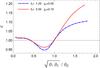 |
Fig. 9 Radial dependence of the axis ratio ϵ. In the unperturbed case the isodensity contours are circular, i.e., |


5. Characterization of the modified mass distribution
The SPT leads to a modified deflection angle of the lens which yields exactly the same astrometric and photometric observational properties as the original mass distribution. For those modified profiles for which a deflection potential can be found such that the differences between the corresponding Δα is sufficiently small, the modified surface mass density provides a viable alternative to the original mass model κ of the lens. In this section we want to consider a diagnostic for the change of the mass profile, both regarding the radial slope and the angular structure of the lens. Since the strong lensing properties of the lens can only be probed in the inner part of the mass distribution, we will apply these diagnostics only to those regions where multiple images can occur, i.e., | θ | ≲ 2θE.
5.1. Radial mass profile
The SPT changes the radial mass profile of the lens. We consider situations in which the original lens is described by a “simple” mass distribution, i.e., an NIS. Combined with a “mild” SPT the resulting remains simple, e.g., still shows closed, concentric isodensity contours.
The mass-sheet transformation is a special case of the SPT, and it is well known that the MST changes the radial profile of the lens. In order to highlight the new feature of the SPT not contained in the MST, we aim at a measure for the radial profile which is invariant under the MST. The MST transforms all derivatives of κ by a constant factor λ, hence it leaves the ratio of derivatives unchanged. Consequently, one possible diagnostic for the effect of the SPT is the radial profile of such ratios, e.g., ⟨κ⟩′′/⟨κ⟩′.
In particular, if the original mass profile is a power law, ⟨κ⟩(θ) ∝ θ− s, then we have θ ⟨κ⟩′′/⟨κ⟩′ = −(s + 1); hence, any deviation from this constant value indicates the effect of the SPT on the modified mass profile . However, if there is no analytical expression of κ and  , the ratio of derivatives is very sensitive to numerical noise, and therefore of little practical interest. We therefore consider hereafter alternative tests.
Noting that the MST yields a multiplication of 1−κ(θ) by λ, the ratio 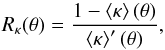 (33)is well defined for monotonically decreasing mass profiles and invariant under the MST. Figure 10 shows Rκ for the NIS and various SPT transformed models. The variations of Rκ are particularly significant above one Einstein radius, in regions where the SPT-transformed profiles deviate also more strongly from the original profile. Despite the fact that deviates from κorginal by more than 20% within θE when f2 = 1.2 (Fig. 8), the most extreme changes of Rκ(θ) reach no more than ~10% within one Einstein radius. As expected, Rκ deviates more strongly from the original profile when | f2 | is large. Negative values of f2 (not shown) are qualitatively similar (but mirrored w.r.t.
  ) to the situation encountered for positive f2. However, at radii θ ~ 1.2 θE, stops being monotonically decreasing, and Rκ diverges.
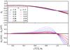 |
Fig. 10 Top: quantity Rκ(θ) (Eq. (33)) calculated for an NIS with external shear γp (cf. Sect. 4; solid black) and for various SPT-transformed models with SPT of the form 1 + f2/ 2 (β/θE)2 (Eq. (28)). The range of positive values of f2 allowed by | Δ αmax | < 5 × 10⁻³θE (Fig. 4) is explored for two different choices of the shear: γp = 0.05 (blue) and γp = 0.1 (red). While Rκ is conserved under an MST, it is not under an SPT, with deviation that can reach tens of percents. Bottom: for each curve of the top panel, we show the difference between Rκ of the original NIS model and of the SPT transformed model. |
Another possibility to characterize the radial profile change is through the aperture mass (see Schneider 1996). Consider a function 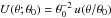 such that u(x) is non-zero only for x ≤ 1; hence, θ0 characterizes the range of support of U(θ;θ0). Furthermore, we require that the filter function U has a vanishing two-dimensional integral over its support, which means that
  Then we define the aperture mass as
  (34)The mass-sheet transformation (1) leads to multiplication of Map by a factor λ, whereas the additive term in Eq. (1) drops out, due to the compensated nature of the filter function U. Thus, if we consider the ratio of the aperture mass for two different scale lengths θ0, the factor λ drops out, and this ratio Map(θ1) /Map(θ2) is invariant under the MST.
Consider again a power-law density profile, ⟨κ⟩(θ) = (1−s/ 2)(θ/θE)− s, with 0 <s< 2, where θE is the Einstein radius in case of axi-symmetry. Then,  and Map(θ1) /Map(θ2) = (θ1/θ2)− s. We thus define the effective slope
  (35)so that for a mass profile of the form ⟨κ⟩(θ) = a + bθ− s, seff = s.
One can think of a number of appropriate weight functions u(x) and aperture scales θi to characterize the modified mass profile. The simplest form would be the sum of two delta functions, u(x) = δ(x−x0)−x0δ(x−1), with x0< 1, for which Map(θ0) = 2πx0[⟨κ⟩(x0θ0)−⟨κ⟩(θ0)]. Furthermore, choosing θ2 = θ1/x0, the ratio of aperture masses becomes  (36)In the case of (1−x0) ≪ 1, the expression (35) becomes
 ![Mathematical equation: \begin{equation} s_{\rm eff}=-1-\frac{\theta_1 \ave{\kappa}''(\theta_1)} {\ave{\kappa}'(\theta_1)} +{\cal O}([1-x_0]^2). \end{equation}](/articles/aa/full_html/2017/05/aa29048-16/aa29048-16-eq260.png) (37)Hence, we see that in this case seff depends just on the ratio of second to first derivative, and reduces to s for a power-law mass profile with slope s.
(37)Hence, we see that in this case seff depends just on the ratio of second to first derivative, and reduces to s for a power-law mass profile with slope s.
More practical choices of u would be such that the profile is probed over an annulus around the Einstein radius θE. For example, one could use the compensated filter function  (38)Figure 11 shows Map as a function of θ0, fixing x0 = 1/2 in Eq. (38). As expected, for two profiles transformed into each other via an MST, the ratio of aperture masses is independent of θ0 and equals λ. Conversely, Map(θ0) of the SPT-transformed profiles intersects the aperture mass “function” of the original profile (i.e. NIS), and the ratio between the two curves changes with θ0. The radius at which the curves intersects is almost independent of the value of f2. This can easily be deduced from the apparent self-similarity of the SPT-transformed mass density profiles (Fig. 8) for various values of f2.
Figure 11 motivates a choice of radii corresponding to extrema of Map(θ0) to calculate aperture mass ratios, such as θ1 = 2 θE and θ2 = θE. Then, Map(θ1) will probe the annulus θE<θ< 2 θE, while for θ2 ~ θE the annulus 0.5 θE ≤ θ ≤ θE would be probed. Figure 12 shows normalized aperture mass ratios Map(θ1) /Map(θ2) for the various SPT-transformed profiles studied in the previous section. We see that larger aperture mass ratios are found for larger values of f2. In addition, the ratio depends only weakly of the shear amplitude γp, which means that the radial deformation of the mass profile produced by the SPT is mostly governed by the amplitude of f2.
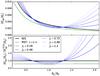 |
Fig. 11 Top: Map(θ0) (Eq. (34)) as a function of the “aperture” θ0. The filter function u(x) defined by Eq. (38), using x0 = 0.5, has been used such that for Map(θ0), the annulus [θ0/ (2θE),θ0/θE] is probed. The black curve shows Map for the NIS profile and the blue curves for the SPT-transformed profiles with γp = 0.05 and various values of f2. The green curve shows Map(θ0) for an MST transformed version of the NIS profile. Bottom: ratio between Map derived for the various transformed profiles and for the original NIS profile. |
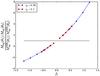 |
Fig. 12 Ratios of aperture mass between θ1 = 2 θE and θ2 = θE for SPT-transformed profiles with various values of f2. The ratios of aperture masses are normalized by the corresponding aperture ratios estimated for the original NIS profile (horizontal bar). The blue diamonds are for a shear γp = 0.05, and the red squares when γp = 0.1. |
5.2. A specific lens model
Here, we apply the previous tests to three mass density profiles studied in SS13 and SS14, and used in those papers to illustrate degeneracies produced by the MST and the SPT. The reference model is a composite model constituted of the sum of a (spherically symmetric) Hernquist component to describe the baryonic component, and a (spherical) generalized Navarro-Frank-White (gNFW) density profile to describe the dark matter component of the galaxy. In addition, an external shear of amplitude γp = 0.1 is considered. Complex sets of lensed images from an ensemble of sources were generated with that model, and found to be all equally well reproduced by two (single) power-law profiles: a global power law, with an almost isothermal density slope γ′ = 1.98 (hereafter model M1), and a local power-law profile with a core radius θc = 0.1′′ and a slope γ′= 2.2 (hereafter model M2). We have applied the tests introduced in the previous subsection to these profiles to identify the nature of the degeneracy between the models. Figure 13 shows the difference Rκ between the original profile and transformed ones, i.e., ΔRκ = Rκ(original)−Rκ(transformed). For comparison, we also show ΔRκ obtained for an SPT with f2 = 0.11. This figure suggests that indeed, this degeneracy is similar to an SPT.
The other diagnostic we present consists in calculating the aperture mass Map of the profiles. Figure 14 shows Map as a function of θ0. In addition to the aperture mass calculated for the individual profiles, we also show the aperture mass corresponding to two different MST-transformed mass density profiles. As explained in SS13, model M1 is close to an MST transformed version of the composite model4 with λ = 0.84. On the other hand, Fig. 4 of SS14 shows that the MST contribution to M2 corresponds to λ = 0.932. Figure 14 is qualitatively similar to Fig. 11 but there is an offset of Map for M1 and M2 compared to the composite model. The reason is probably that the M1 and M2 profiles are transformed versions of the composite model via both an MST and an SPT. The MST contribution with λ = 0.84 is larger for M1 than for M2, for which λ ~ 0.93.
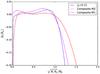 |
Fig. 13 Difference between Rκ calculated for three different pairs of profiles: In blue, an NIS and an SPT-transformed model with f2 = 0.11 and γp = 0.1; in magenta, a composite Hernquist+gNFW model and a power-law model (M1); in red, Hernquist+gNFW model and a cored power-law model (M2). The shape of ΔRκ for the models presented in SS13 and SS14 are qualitatively similar to that observed for the fiducial SPT model presented in Sect. 4. |
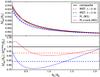 |
Fig. 14 Top: Map(θ0) (Eq. (34)) as a function of θ0, for the composite Hernquist+gNFW model (black), for the power law model M1 (blue), and the cored power-law M2 (red). Dashed red (blue) profile shows Map(θ0) for an MST transformed version of the composite model with λ = 0.93 (resp. 0.84). Bottom: ratio of Map(θ0) between the “transformed” models and the composite. The dashed curves correspond to MST-transformed versions of the composite model, and represent the contribution of the MST to M1 and M2. The solid red and blue curves suggest that the remaining of the degeneracy can be associated with an SPT. |
6. Discussion – Implications of the SPT for strong lensing
In this paper we have studied several aspects of the SPT, an invariance transformation of the deflection angle that leaves all multiple images properties of gravitational lenses invariant. The central question, of whether there exists a gravitational lensing potential which gives rise to a deflection angle sufficiently close to the SPT-transformed one (which in general is not curl free) has been explored for a particular class of lens models, namely an NIS with external shear and an SPT given as a radial stretching of the source plane. The radial stretching deformation was chosen such that the classical MST did not contribute in altering the original deflection since we are only interested in higher-order effects that go beyond the well known MST. This example has shown that, for a large range of parameters pairs (external shear and distortion parameter of the radial stretching) there indeed exist lensing potentials whose associated deflection is sufficiently close to the one obtained from the SPT that these two cannot be distinguish observationally. We conducted this study by formulating an action as the integral over the squared difference of these two deflection angles, yield a Neumann problem. We gave a detailed description of how this problem can be solved; these methods are expected to be useful for future theoretical studies and applications of the SPT.
We have considered only one criterion for the validity of an SPT, namely that the corresponding gradient deflection field does not deviate from the SPT-transformed deflection by more than 5 × 10⁻³θE. Changing this observationally motivated limit to a different value will modify the space of allowed parameter combinations. For the example considered here, we expect that the allowed range of the stretching parameter f2 for a given external shear will be proportional to the allowed maximum deviation of these two deflection angles.
We point out that our method of obtaining a gradient deflection law in form of the variational principle (6) does not necessarily yield an “optimal” modified deflection. As briefly discussed in Sect. 3.1, one could imagine alternative constraints for finding a gradiant deflection “close to ”. In particular, finding a gradient field whose maximum deviation from is minimized over the region of relevance would be a promising ansatz which, however, is analytically challenging, if at all doable. Nevertheless, the solution obtained in this paper yields valuable insight in the freedom of lens model choices offered by the SPT.
The properties of the mass distribution resulting from an SPT were also studied in detail. In contrast to the MST, which is a special case of an SPT, the more general SPT gives rise to non-monotonic changes in the radial mass profile, and to the generation of a finite ellipticity even if the original mass distribution was axi-symmetric. Hence, the SPT offers a much larger range of mass profile modifications which leave all strong lensing observables invariant, than does the MST. This more complex class of invariance transformation is of particular interest because it may be of great relevance when trying to fit real lens system (which are expected to have a rather complex mass profile; see, e.g., Xu et al. (2016) with simple lens models. The fact that simple mass models yield satisfactory fits even in cases with a rich observed image structure may be a consequence of some SPT which transforms the deflection of the true mass distribution into that of a simple mass model. Ignoring the potential complexity of the real mass distribution, and thus the possibility that the SPT may be acting, may lead to biases in estimates of physical parameters of the lens system.
We have defined several diagnostic quantities which can distinguish a general SPT from a pure MST. Applying these diagnostics to the special case of nearly degenerate lens models studies in two earlier papers, we conclude that this degeneracy can to a large degree be accounted by an MST, but that a non-negligible contribution comes from a more general SPT. Hence, an SPT has been found “empirically”, even before the concept of the SPT was developed. In that sense, the SPT is not just a “theoretical possibility” for obtaining different but observationally equivalent mass models, but describes degeneracies which actually occur in real lens modeling.
Although time delay ratios stay constant.
E.g., the last term in Eq. (21) would be missing.
We note that this extrapolation has to be carried out with the deflection angle, not with the potential, since the latter is determined only up to an additive constant – which may depend on the iteration step m and the number of grid points.
In SS13, we reported λ = βfid/βPL = 1.19, which is the inverse of λ used here that is such that κPL = λκfid + (1−λ).
Acknowledgments
We would like to thank Bastian Orthen for valuable discussions, Olivier Wertz for valuable comments on this paper, and the referee, Matthias Bartelmann, for his constructive comments and advice. Part of this work was supported by the German Deutsche Forschungsgemeinschaft, DFG project numbers SL 172/1-1 and SCHN 342/13-1. Sandra Unruh is a member of the International Max Planck Research School (IMPRS) for Astronomy and Astrophysics at the Universities of Bonn and Cologne. Dominique Sluse is supported by a Back to Belgium grant from the Belgian Federal Science Policy (BELSPO).
References
- Bartelmann, M. 2010, Class. Quantum Gray., 27, 233001 [NASA ADS] [CrossRef] [Google Scholar]
- Bradač, M., Schneider, P., Lombardi, M., et al. 2004, A&A, 423, 797 [NASA ADS] [CrossRef] [EDP Sciences] [Google Scholar]
- Coe, D., Fuselier, E., Benítez, N., et al. 2008, ApJ, 681, 814 [NASA ADS] [CrossRef] [Google Scholar]
- Diego, J. M., Sandvik, H. B., Protopapas, P., et al. 2005, MNRAS, 362, 1247 [NASA ADS] [CrossRef] [Google Scholar]
- Falco, E. E., Gorenstein, M. V., & Shapiro, I. I. 1985, ApJ, 289, L1 [Google Scholar]
- Hezaveh, Y. D., Marshall, P. J., & Blandford, R. D. 2015, ApJ, 799, L22 [NASA ADS] [CrossRef] [Google Scholar]
- Kochanek, C. S. 2006, in Saas-Fee Advanced Course 33: Gravitational Lensing: Strong, Weak and Micro, eds. G. Meylan, P. Jetzer, P. North, et al., 91 [Google Scholar]
- Kochanek, C. S., & Dalal, N. 2004, ApJ, 610, 69 [NASA ADS] [CrossRef] [Google Scholar]
- Liesenborgs, J., & De Rijcke, S. 2012, MNRAS, 425, 1772 [NASA ADS] [CrossRef] [Google Scholar]
- Mao, S., & Schneider, P. 1998, MNRAS, 295, 587 [NASA ADS] [CrossRef] [Google Scholar]
- Metcalf, R. B. 2005, ApJ, 629, 673 [NASA ADS] [CrossRef] [Google Scholar]
- Press, W. H., Teukolsky, S. A., Vetterling, W. T., & Flannery, B. P. 1996, Numerical recipes in C (New York: Cambridge University Press) [Google Scholar]
- Saha, P., & Williams, L. L. R. 1997, MNRAS, 292, 148 [NASA ADS] [CrossRef] [Google Scholar]
- Schneider, P. 2006, in Saas-Fee Advanced Course 33: Gravitational Lensing: Strong, Weak and Micro, eds. G. Meylan, P. Jetzer, P. North, et al., 1 [Google Scholar]
- Schneider, P., & Sluse, D. 2013, A&A, 559, A37 [NASA ADS] [CrossRef] [EDP Sciences] [Google Scholar]
- Schneider, P., & Sluse, D. 2014, A&A, 564, A103 [NASA ADS] [CrossRef] [EDP Sciences] [Google Scholar]
- Seitz, S., & Schneider, P. 2001, A&A, 374, 740 [NASA ADS] [CrossRef] [EDP Sciences] [Google Scholar]
- Winn, J. N., Rusin, D., & Kochanek, C. S. 2004, Nature, 427, 613 [NASA ADS] [CrossRef] [Google Scholar]
- Xu, D. D., Mao, S., Cooper, A. P., et al. 2010, MNRAS, 408, 1721 [NASA ADS] [CrossRef] [Google Scholar]
- Xu, D. D., Mao, S., Cooper, A. P., et al. 2012, MNRAS, 421, 2553 [NASA ADS] [CrossRef] [Google Scholar]
- Xu, D., Sluse, D., Schneider, P., et al. 2016, MNRAS, 456, 739 [NASA ADS] [CrossRef] [Google Scholar]
Appendix A: Practical integration of Eq. (22) in a circular region
Calculating the deflection angle  in Eq. (18) by integrating the product
  over the circle poses a challenge, due to the pole of the first term in Eq. (21). To integrate over this pole, polar coordinates centered on the pole position ϑ need to be chosen. This can be done by a translation of the integration variable to x = θ−ϑ, and integrating in the polar coordinates of x. However, the integration range of the polar angle will depend on | x |, according to the geometrical overlap of circles centered on the origin and those centered on θ.
A better method is obtained by a conformal mapping of the form  (A.1)where we now use complex notation, i.e., x, ϑ and θ are complex numbers with components ϑ = ϑ1 + iϑ2 etc. and an asterisk denotes complex conjugation. This conformal mapping maps the circle | θ | <R onto the unit circle | x | < 1, and the singularity point θ = ϑ is mapped onto the origin x = 0. For example, setting θ = Reiϕ, we get
  from which it is immediately seen that | x | = 1. The inverse of the transformation (A.1) is readily obtained,
  (A.2)from which one can easily check that the unit circle | x | = 1 is mapped onto the circle | θ | = R. In components, Eq. (A.2) reads
 ![Mathematical equation: \appendix \setcounter{section}{1} \begin{eqnarray} \theta_1&=&\frac{R x_1+\vt_1(1+|x|^2)+[x_1(\vt_1^2-\vt_2^2)+2\vt_1\vt_2x_2]/R} {1+2\vc\vt\cdot\vc x/R+|\vc\vt|^2 |\vc x|^2/R^2}, \nonumber \\ \theta_2&=&\frac{R x_2+\vt_2(1+|x|^2)+[2\vt_1\vt_2 x_1 - x_2(\vt_1^2-\vt_2^2)]/R} {1+2\vc\vt\cdot\vc x/R+|\vc\vt|^2 |\vc x|^2/R^2}\cdot \end{eqnarray}](/articles/aa/full_html/2017/05/aa29048-16/aa29048-16-eq313.png) (A.3)The Jacobi determinant of the transformation x → θ, needed for the integration, is
(A.3)The Jacobi determinant of the transformation x → θ, needed for the integration, is  (A.4)which is non-zero for all x inside the unit circle and | ϑ | <R. As a sanity check, we calculate the area of the circle in the transformed coordinates,
  (A.5)The inner integral yields 2π(R2 + | x | 2 | ϑ | 2)/(R2− | x | 2 | ϑ | 2)3, the outer integral then gives π/ (R2− | ϑ | 2)2, and we re-obtain the area πR2.
In complex notation, the singular term in Eq. (21) reads  yielding
  (A.6)We can check the consistency of this expression by calculating the deflection angle of a uniform disk with surface mass density κ0, which reads
 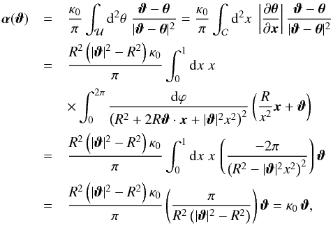 (A.7)as expected.
Appendix B: Proof of the relation (26) for a circular region
In this section we use again the complex notation for two-dimensional vectors, in terms of which the vector field (21) reads 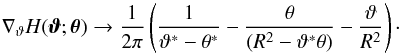 (B.1)Therefore, we obtain for the fields A and Bin the complex expressions
 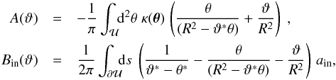 (B.2)where ain = αin·n, defined on the boundary of . We first calculate this product, noting that for a boundary point R eiϕ of the circle, n = eiϕ. Specializing the complex expression for αin as given in Eq. (23) to a point on the boundary, ϑ = Rn, we obtain
 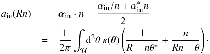 (B.3)We now insert this expression into Eq. (B.2). The integral over the boundary is written as ds = R dϕ = −i R dn/n, and the integral over n extends over the unit circle. With θ = Rn, we then find
 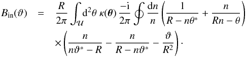 (B.4)The inner integrand is an analytic function of n inside the unit circle, except at the poles at n = 0 and at n = θ/R (ϑ and θ are both inside the circle). Applying the theorem of residue, the integral can thus be evaluated. The first pole yields a contribution −ϑ/R3, whereas the second pole results in the expression
 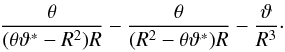 Adding up these two contributions then yields
 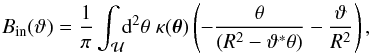 (B.5)which we see agrees with the expression for A in Eq. (B.2). Thus we have shown explicitly that for the kernel function (20), the relation (26) holds.
Appendix C: Conservation of mass inside the Einstein radius under SPT
Starting from (32) we can infer the mass inside the Einstein radius by performing an integration up to θE. First, we consider the case of an axisymmetric lens model, i.e., γp = 0. Thus, the integral we have to solve is ![Mathematical equation: \appendix \setcounter{section}{3} \begin{eqnarray} \hat{M}_{\gp=0}(\le\tE) &=& 2 \int_0^{\tE} \d \theta \; \theta \, \khat(\theta) \nonumber\\ = M(\le\tE) &&+ f_2 \int_0^{\tE} \d \theta \; \theta^3 ( 1 - \kbar )^2 [3 (\kappa - \kbar) - 2 (1 - \kbar)]. \label{eq:MintE} \end{eqnarray}](/articles/aa/full_html/2017/05/aa29048-16/aa29048-16-eq342.png) (C.1)To show that mass is conserved in case of an SPT, the integral in Eq. (C.1) has to vanish for arbitray mass profiles κ(θ). We note that
(C.1)To show that mass is conserved in case of an SPT, the integral in Eq. (C.1) has to vanish for arbitray mass profiles κ(θ). We note that  is given by
 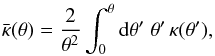 (C.2)from which follows
  (C.3)
(C.3)
of which we will make use in the next step. We perform an integration by parts for the last term in Eq. (C.1), ![Mathematical equation: \appendix \setcounter{section}{3} \begin{eqnarray} 2 \int_0^{\tE} \d \theta \; \theta^3 (1 - \kbar)^3 &=& \left[ 2 \frac{\theta^4}{4} (1-\kbar)^3 \right]^{\tE}_0 + 2 \int_0^{\tE} \d \theta \; \frac{\theta^4}{4} \, 3 (1-\kbar)^2 \kbar' \nonumber\\ &= &3 \int_0^{\tE} \d \theta \; \theta^3 \, (1-\kbar)^2 (\kappa - \kbar), \end{eqnarray}](/articles/aa/full_html/2017/05/aa29048-16/aa29048-16-eq346.png) (C.4)where we used
(C.4)where we used  . This result matches exactly the first term in the integral of Eq. (C.1). Hence, in the case γp = 0 the mass inside the Einstein ring is conserved under an SPT.
Next, we consider the case for γp ≠ 0. To integrate over the Einstein radius we make use of the result above, i.e.,  . Since the two latter parts of Eq. (32) are proportional to cos(2φ) or cos(4φ), respectively, they do not contribute to an integral over a circular area. Hence, we calculate
 ![Mathematical equation: \appendix \setcounter{section}{3} \begin{eqnarray} \hat{M}(\le\tE) &=& 2 \int_0^{\tE} \d \theta \; \theta \khat(\theta) \nonumber\\ &= &M(\le\tE) + f_2 \gp^2 \int_0^{\tE} \d \theta \; \theta^3 [2 (\kappa - \kbar) - 4 (1 - \kbar)]. \label{eq:MintEfull} \end{eqnarray}](/articles/aa/full_html/2017/05/aa29048-16/aa29048-16-eq353.png) (C.5)Again, we consider first the last term in the integral of Eq. (C.5), and we make use of Eq. (C.3) and
(C.5)Again, we consider first the last term in the integral of Eq. (C.5), and we make use of Eq. (C.3) and  . Then, we obtain
 ![Mathematical equation: \appendix \setcounter{section}{3} \begin{eqnarray} 4 \int_0^{\tE} \d \theta \; \theta^3 (1 - \kbar) &=& \left[ 4 \frac{\theta^4}{4} (1-\kbar) \right]^{\tE}_0 + 4 \int_0^{\tE} \d \theta \; \frac{\theta^4}{4} \, \kbar' \nonumber\\ &=& 2 \int_0^{\tE} \d \theta \; \theta^3 \, (\kappa - \kbar). \end{eqnarray}](/articles/aa/full_html/2017/05/aa29048-16/aa29048-16-eq355.png) (C.6)This matches the first term in the integral exactly and therefore, the integral vanishes. Thus, also in the case of an external shear γp the mass enclosed in the Einstein ring is conserved, i.e.,
(C.6)This matches the first term in the integral exactly and therefore, the integral vanishes. Thus, also in the case of an external shear γp the mass enclosed in the Einstein ring is conserved, i.e.,  , independent of the choice of mass model κ.
All Figures
|
Fig. 1 Illustration of the source position transformation. A source at β causes multiple images θ in the lens plane under the deflection law α. The same multiple images are obtained from a source at |
| In the text | |
|
Fig. 2 Illustration of the extrapolation method used in the SOR method (Sect. 3.2) to calculate |
| In the text | |
|
Fig. 3 Maximum difference of |
| In the text | |
|
Fig. 4 Values of |Δα| max are plotted against the parameters f2 from (28) and external shear strength γp. The colored region indicates allowed pairs of parameters that fulfill the |Δα| < 5 × 10⁻³θE-criterion. For obtaining this figure, we used the SOR method. |
| In the text | |
|
Fig. 5 Values of |
| In the text | |
|
Fig. 6 For every allowed combination f2 and γp the values of | Δα | max (Fig. 4) are plotted against |
| In the text | |
|
Fig. 7 Map of | Δα(θ) | is shown for f2 = 0.55 and γp = 0.1. The strong changes in the corners, i.e. θ > 2 θE, are biased by large numerical uncertainty and should be neglected. |
| In the text | |
|
Fig. 8 Upper panel shows the mass profile of the original NIS lens (solid curve), and that of three SPT-transformed lenses, with parameters f2 and γp indicated by the labels. For all of these three models, Δαmax ≈ εacc = 5 × 10⁻³θE. Since the transformed mass distributions have a finite ellipticity, the density is plotted as a function of the geometric mean of the major and minor semi-axis of the best-fitting ellipse to an isodensity contour, except for the case with negative f2, for which the outer isodensity contours are not closing around the lens center; in this special case, the x-axis corresponds to the θ1-axis. The convergence changes up to 28% for radii smaller than 1 θE, radii larger than that show a significantly smaller convergence for a positive f2. Negative f2 show an essentially mirrored behavior compared to positive f2. This leads to convergence |
| In the text | |
|
Fig. 9 Radial dependence of the axis ratio ϵ. In the unperturbed case the isodensity contours are circular, i.e., |
| In the text | |
|
Fig. 10 Top: quantity Rκ(θ) (Eq. (33)) calculated for an NIS with external shear γp (cf. Sect. 4; solid black) and for various SPT-transformed models with SPT of the form 1 + f2/ 2 (β/θE)2 (Eq. (28)). The range of positive values of f2 allowed by | Δ αmax | < 5 × 10⁻³θE (Fig. 4) is explored for two different choices of the shear: γp = 0.05 (blue) and γp = 0.1 (red). While Rκ is conserved under an MST, it is not under an SPT, with deviation that can reach tens of percents. Bottom: for each curve of the top panel, we show the difference between Rκ of the original NIS model and of the SPT transformed model. |
| In the text | |
|
Fig. 11 Top: Map(θ0) (Eq. (34)) as a function of the “aperture” θ0. The filter function u(x) defined by Eq. (38), using x0 = 0.5, has been used such that for Map(θ0), the annulus [θ0/ (2θE),θ0/θE] is probed. The black curve shows Map for the NIS profile and the blue curves for the SPT-transformed profiles with γp = 0.05 and various values of f2. The green curve shows Map(θ0) for an MST transformed version of the NIS profile. Bottom: ratio between Map derived for the various transformed profiles and for the original NIS profile. |
| In the text | |
|
Fig. 12 Ratios of aperture mass between θ1 = 2 θE and θ2 = θE for SPT-transformed profiles with various values of f2. The ratios of aperture masses are normalized by the corresponding aperture ratios estimated for the original NIS profile (horizontal bar). The blue diamonds are for a shear γp = 0.05, and the red squares when γp = 0.1. |
| In the text | |
|
Fig. 13 Difference between Rκ calculated for three different pairs of profiles: In blue, an NIS and an SPT-transformed model with f2 = 0.11 and γp = 0.1; in magenta, a composite Hernquist+gNFW model and a power-law model (M1); in red, Hernquist+gNFW model and a cored power-law model (M2). The shape of ΔRκ for the models presented in SS13 and SS14 are qualitatively similar to that observed for the fiducial SPT model presented in Sect. 4. |
| In the text | |
|
Fig. 14 Top: Map(θ0) (Eq. (34)) as a function of θ0, for the composite Hernquist+gNFW model (black), for the power law model M1 (blue), and the cored power-law M2 (red). Dashed red (blue) profile shows Map(θ0) for an MST transformed version of the composite model with λ = 0.93 (resp. 0.84). Bottom: ratio of Map(θ0) between the “transformed” models and the composite. The dashed curves correspond to MST-transformed versions of the composite model, and represent the contribution of the MST to M1 and M2. The solid red and blue curves suggest that the remaining of the degeneracy can be associated with an SPT. |
| In the text | |
Current usage metrics show cumulative count of Article Views (full-text article views including HTML views, PDF and ePub downloads, according to the available data) and Abstracts Views on Vision4Press platform.
Data correspond to usage on the plateform after 2015. The current usage metrics is available 48-96 hours after online publication and is updated daily on week days.
Initial download of the metrics may take a while.