| Issue |
A&A
Volume 600, April 2017
|
|
|---|---|---|
| Article Number | L10 | |
| Number of page(s) | 9 | |
| Section | Letters | |
| DOI | https://doi.org/10.1051/0004-6361/201629754 | |
| Published online | 04 April 2017 | |
ALMA survey of massive cluster progenitors from ATLASGAL
Limited fragmentation at the early evolutionary stage of massive clumps⋆
1 Max Planck Institute for Radioastronomy, Auf dem Hügel 69, 53121 Bonn, Germany
e-mail: This email address is being protected from spambots. You need JavaScript enabled to view it.
2 OASU/LAB-UMR5804, CNRS, Université Bordeaux, allée Geoffroy Saint-Hilaire, 33615 Pessac, France
3 Institut de Planétologie et d’Astrophysique de Grenoble, Univ. Grenoble Alpes – CNRS-INSU, BP 53, 38041 Grenoble Cedex 9, France
4 Laboratoire AIM Paris Saclay, CEA-INSU/CNRS-Université Paris Diderot, IRFU/SAp CEA-Saclay, 91191 Gif-sur-Yvette, France
5 Max Planck Institute for Astronomy, Königstuhl 17, 69117 Heidelberg, Germany
6 Departamento de Astronomía, Universidad de Chile, Casilla 36-D, Santiago, Chile
7 Univ. Lyon, ENS de Lyon, Univ Lyon1, CNRS, Centre de Recherche Astrophysique de Lyon UMR5574, F-69007, Lyon, France
8 IRAM, 300 rue de la piscine, 38406 Saint-Martin-d’ Hères, France
9 School of Physics and Astronomy, University of Exeter, UK
10 Jodrell Bank Centre for Astrophysics, School of Physics and Astronomy, The University of Manchester, Manchester, M13 9PL, UK
11 Astrophysics Research Institute, Liverpool John Moores University, UK
12 Instituto de Radioastronomía y Astrofísica, Universidad Nacional Autónoma de México, Mexico
13 School of Physics & Astronomy, Cardiff University, UK
14 Departments of Astronomy and Physics, University of Florida, USA
15 European Southern Observatory, Karl-Schwarzschild-Strasse 2, 85748 Garching, Germany
16 INAF–Osservatorio Astrofisico di Arcetri, Largo E. Fermi 5, 50125 Firenze, Italy
17 IAPS–INAF, Via Fosso del Cavaliere, 100, 00133 Rome, Italy
18 School of Physical Sciences, University of Kent, Ingram Building, Canterbury, Kent CT2 7NH, UK
Received: 20 September 2016
Accepted: 1 March 2017
Abstract
The early evolution of massive cluster progenitors is poorly understood. We investigate the fragmentation properties from 0.3 pc to 0.06 pc scales of a homogenous sample of infrared-quiet massive clumps within 4.5 kpc selected from the ATLASGAL survey. Using the ALMA 7 m array we detect compact dust continuum emission towards all targets and find that fragmentation, at these scales, is limited. The mass distribution of the fragments uncovers a large fraction of cores above 40 M⊙, corresponding to massive dense cores (MDCs) with masses up to ~400 M⊙. Seventy-seven percent of the clumps contain at most 3 MDCs per clump, and we also reveal single clumps/MDCs. The most massive cores are formed within the more massive clumps and a high concentration of mass on small scales reveals a high core formation efficiency. The mass of MDCs highly exceeds the local thermal Jeans mass, and we lack the observational evidence of a sufficiently high level of turbulence or strong enough magnetic fields to keep the most massive MDCs in equilibrium. If already collapsing, the observed fragmentation properties with a high core formation efficiency are consistent with the collapse setting in at parsec scales.
Key words: stars: formation / stars: massive / submillimeter: ISM
Full Table A.1 is only available at the CDS via anonymous ftp to cdsarc.u-strasbg.fr (130.79.128.5) or via http://cdsarc.u-strasbg.fr/viz-bin/qcat?J/A+A/600/L10
© ESO, 2017
1. Introduction
The properties and evolution of massive clumps hosting the precursors of the highest mass stars currently forming in our Galaxy are poorly known. Massive clumps at an early evolutionary phase,thus, prior to the emergence of luminous massive young stellar objects and UC-H II regions, are excellent candidates to host high-mass protostars in their earliest stages (e.g. Zhang et al. 2009; Bontemps et al. 2010; Csengeri et al. 2011a,b; Palau et al. 2013; Sánchez-Monge et al. 2013). Large samples have only recently been identified based on large area surveys (e.g. Butler & Tan 2012; Tackenberg et al. 2012; Traficante et al. 2015; Svoboda et al. 2016; Csengeri et al. 2017), which show that the early evolutionary stages are short lived (e.g. Motte et al. 2007; Csengeri et al. 2014), as star formation proceeds rapidly. Using the Atacama Large Millimeter/submillimeter Array (ALMA), here we present the first results of a statistical study of early stage fragmentation to shed light on the physical processes at the origin of high-mass collapsing entities and to search for the youngest precursors of O-type stars.
2. The sample of infrared quiet massive clumps
Based on a flux limited sample of the 870 μm APEX Telescope LArge Survey of the GAlaxy (ATLASGAL; Schuller et al. 2009; Csengeri et al. 2014), Csengeri et al. (2017) identified the complete sample of massive infrared quiet clumps withthe highest peak surface density (Σcl ≥ 0.5 g cm-2)1 and low bolometric luminosity, Lbol< 104 L⊙, corresponding to the ZAMS luminosity of a late O-type star. Their large mass reservoir and low luminosity suggest that infrared quiet massive clumps correspond to the early evolutionary phase; some of them already exhibit signs of ongoing (high-mass) star formation, such as EGOs and Class II methanol masers. Here we present the sample of 35 infrared quiet massive clumps located within d ≤ 4.5 kpc, which could be conveniently grouped on the sky as targets for ALMA. They cover 70% of all the most massive and nearby infrared quiet clumps from Csengeri et al. (2017) and are thus a representative selection of a homogenous sample of early phase massive clumps in the inner Galaxy.
Summary of observations.
3. Observations and data reduction
We present observations carried out in Cycle 2 with the ALMA 7 m array using 9 to 11 of the 7 m antennas with baselines ranging between 8.2 m (9.5kλ) to 48.9 m (53.4kλ). We used a low-resolution wide-band set-up in Band 7, yielding 4 × 1.75 GHz effective bandwidth with a spectral resolution of 976.562 kHz. The four basebands were centred on 347.331, 345.796, 337.061, and 335.900 GHz, respectively. The primary beam at this frequency is 28.9′′. Each source was observed for ~5.4 min in total. The system temperature, Tsys, varies between 100−150 K. The targets were split into five observing groups according to Galactic longitude (Table 1).
The data was calibrated using standard procedures in CASA 4.2.1. To obtain line-free continuum images, we first identified the channels with spectral lines towards each source and, excluding these, averaged the remaining channels. We used a robust weight of 0.5 for imaging and the CLEAN algorithm for deconvolution and corrected for the primary beam attenuation. The synthesized beam varies between 3.5′′ to 4.6′′ taking the geometric mean of the major and minor axes.We measured the noise in an emission free area close to the centre of the maps including the side lobes. The achieved median rms noise level is 54 mJy/beam and varies among the targets owing to a combination of restricted bandwidth available for continuum, dynamic range, or mediocre observing conditions. In particular for groups 4 and 5, the observations were carried out at low elevation resulting in an elongated beam and poor uv sampling.The observing parameters per group are summarized in Table 1 and those for each source in Table A.1.
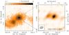 |
Fig. 1 Left: Clump-scale view by ATLASGAL of an example source. Right: Line-free continuum emission at 345 GHz by the ALMA 7 m array. Contours start at 7σrms noise and increase in a logarithmic scale. White crosses indicate the extracted sources (see Table A.1). The synthesized beam is shown in the lower left corner. |
4. Results and analysis
Compact continuum emission is detected towards all clumps (see Fig. 1 for an example, and Fig. A.1 for all targets). We find sources that stay single (~14%) at our resolution and sensitivity. Fragmentation is, in fact, limited towards the majority of the sample; 45% of the clumps host up to two, while 77% host up to three compact sources. Only a few clumps host more fragments.
We identify and measure the parameters of the compact sources using the Gaussclumps task in GILDAS2, which performs a 2D Gaussian fitting. A total number of 124 fragments down to a ~7 σrms noise level are systematically identified within the primary beam, where the noise is measured towards each field. This gives on average  sources per clump corresponding to a population of cores at the typically achieved physical resolution of ~0.06 pc.
We can directly compare the integrated flux in compact sources seen by the ALMA 7 m array with the ATLASGAL flux densities measured over the primary beam of the array as both datasets have similar centre frequencies3. We recover between 16−47% of the flux and the rest of the emission is filtered above the typically 19′′ largest angular scale sensitivity of the ALMA 7 m array observations.
To estimate the mass, we assume optically thin dust emission and use the same formula as in Csengeri et al. (2017) as follows: M = S870μmd2κ870μm-1B870μm(Td)-1, where S870μm is the integrated flux density, d is the distance, κ870μm = 0.0185 g cm-2 from Ossenkopf & Henning (1994) accounting for a gas-to-dust ratio of 100, and Bν(Td) is the Planck function. While on the ~0.3 pc scales of clumps Csengeri et al. (2017) adopt Td = 18 K, on smaller scales of cores heating due to the embedded protostar may result in elevated dust temperatures that are poorly constrained. Following the model of Goldreich & Kwan (1974), we estimate Td = 15−38 K for the luminosity range of 102−104 L⊙ at a typical radius of half the deconvolved FWHM size of 0.025 pc. We adopt thus Td = 25 K , which results up to a factor of two uncertainty in the mass estimate.
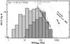 |
Fig. 2 Mass distribution of MDCs within d ≤ 4.5 kpc. The Poisson error of each bin is shown as a grey line above the 10σrms completeness limit of 50 M⊙, the power-law fit is shown in a solid black line. Hashed area shows the distribution of the brightest cores ( |
The extracted cores have a mean mass of ~63 M⊙ corresponding to massive dense cores (MDCs as in Motte et al. 2007) and about 40% of the sample host cores more massive than 150 M⊙. They are, in terms of physical properties, similar to SDC335-MM1 (Peretto et al. 2013), which is here the most massive core with ~400 M⊙ within a deconvolved FWHM size of 0.054 pc 4. In these clumps the second brightest sources are also typically massive, on average 78 M⊙ suggesting a preference to form more massive cores. Except for one clump, no core is detected below 35 M⊙ which is well above the typical detection threshold considering the mean 7σrms mass sensitivity of 11.2 M⊙ at the mean distance of 2.6 kpc, which may indicate a lack of intermediate mass (between 10−40 M⊙) cores. Similar findings have been reported towards a handful of other young massive sources by Bontemps et al. (2010) and Zhang et al. (2015). Clumps with single sources host strictly massive cores with MMDC> 40 M⊙, and about half of these reach the highest mass range of MMDC> 150 M⊙.
We show the mass distribution of cores as ΔN/ Δlog M ~ Mα in Fig. 2 and indicate the 10σrms completeness limit of 50 M⊙, which is set by the highest noise in the poorest sensitivity data. The distribution tends to be flat up to the completeness limit and then shows a decrease at the highest masses. The distribution of  (hatched histogram) shows that the majority of the clumps host at least one massive core, while a few host only at most intermediate mass fragments. The least squares power-law fit to the highest mass bins above the completeness limit gives α = −1.01 ± 0.20. This value is steeper than the distribution of CO clumps (α = −0.6 to − 0.8, Kramer et al. 1998) and tends to be shallower than the low-mass prestellar CMF and the stellar initial mass function (IMF) (α = −1.35−−1.5, André et al. 2010), although at the high-mass end the scatter of the measured slopes is more significant (Bastian et al. 2010). Using Monte Carlo methods we tested the uncertainty of α due to the unknown dust temperature and simulated a range of Td between 10−50 K using a normal distribution with a mean of 25 K and a power-law distribution. We fitted to the slope the same way, as above, and repeated the tests until the standard deviation of the measured slope reached convergence. In good agreement with the observational results,the normal temperature distribution gives αMC = −1.01 ± 0.11 and thus constrains the error of the fit, suggesting an intrinsically shallower slope than the IMF. A power-law temperature distribution in the same mass range with an exponent of − 0.5 could reproduce, however, the slope of the IMF, assuming that the brightest sources are intrinsically warmer. Alternatively, a larger level of fragmentation of the brightest cores on smaller scales could also reconcile our result with the IMF.
5. Discussion
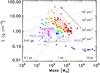 |
Fig. 3 Surface density vs. mass diagram. Coloured dotted lines in different shades show constant radius (green) and nH number density (red; cf. Tan et al. 2014). Coloured large circles show clumps (ATLASGAL), while smaller circles show the cores (ALMA 7 m array), colours scaling from blue to red with increasing |
5.1. Limited fragmentation from clump to core scale
The thermal Jeans mass in massive clumps is low (MJ ~1 M⊙ at  cm-3, T = 18 K), which is expected to lead to a high degree of fragmentation. In contrast, the observed infrared quiet massive clumps exhibit here limited fragmentation with , from clump to core scales. We even find single clumps/MDCs at our resolution. This is intriguing also because these most massive clumps of the Galaxy are expected to form rich clusters. The selected highest peak surface density clumps could therefore correspond to a phase of compactness where the large level of fragmentation to form a cluster has not yet developed.
We find that the mass surface density (Σ) increases towards small scales (Fig. 3, c.f. Tan et al. 2014) corresponding to a high concentration of mass. Eighty percent of the clumps host MDCs above 40 M⊙ and the most massive fragments scale with the mass of their clump. Two models are shown with arrows in Fig. 3: first, clumps with a uniform mass distribution forming low-mass stars correspond to a roughly constant mass surface density and, second, clumps with all the mass concentrated in a single object correspond to n(r) ~ r-2 density profile. The majority of the sources fit the steeper better than uniform density profile.
The early fragmentation of massive clumps thus does not seem to follow thermal processes and shows fragment masses largely exceeding the local Jeans mass (see also Zhang et al. 2009; Bontemps et al. 2010; Wang et al. 2014; Beuther et al. 2015; Butler & Tan 2012). The significant concentration of mass on small scales also manifests in a high core formation efficiency (CFE), which is the ratio of the total mass in fragments and the total clump mass from Csengeri et al. (2017) adopting the same physical parameters (Fig. 4). The CFE suggests an increasing concentration of mass in cores with the average clump volume density ( ); this trend has been seen, although inferred from smaller scales, towards high-mass infrared quiet MDCs in Cygnus-X (Bontemps et al. 2010), low-mass cores in ρ Oph (Motte et al. 1998), and in a sample of infrared bright MDCs (Palau et al. 2013). Although the CFE shows variations at high densities with
  cm-3, exceptionally high CFE of over 50% can only be reached towards the highest average clump densities.
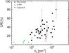 |
Fig. 4 Core formation efficiency vs. average clump density ( |
5.2. Which physical processes influence fragmentation?
What can explain why the thermal Jeans mass does not represent well the observed fragmentation properties in the early stages? A combination of turbulence, magnetic field, and radiative feedback could increase the necessary mass scale for fragmentation. Using the Turbulent Core model (McKee & Tan 2003) for cores with MMDC> 150 M⊙ at the average radius of 0.025 pc, we estimate from their Eq. (18) a turbulent line width of Δvobs ≳ 6 km s-1 at the surface of cores, which is a factor of two higher than the average Δvobs at the clump scale (Wienen et al. 2015). The magnetic critical mass at the average clump density corresponds to Mmag< 400 M⊙ at the typically observed magnetic field values of 1 mG towards massive clumps (e.g. Falgarone et al. 2008; Girart et al. 2009; Cortes et al. 2016; Pillai et al. 2016) following Eq. (2.17) of Bertoldi & McKee (1992). This suggests that moderately strong magnetic fields could explain the large core masses, however, at the high core densities of  cm-3 considerably stronger fields, on the order of B> 10 mG, would be required to keep the most massive cores sub-critical. Although radiative feedback could also limit fragmentation (e.g. Krumholz et al. 2007; Longmore et al. 2011), infrared quiet massive clumps are at the onset of star formation activity and we lack evidence for a potential deeply embedded population of low-mass protostars needed to heat up the collapsing gas.
5.3. Can global collapse explain the mass of MDCs?
The rather monolithic fashion of collapse suggests that fragmentation is already at least partly determined at the clump scale, which would be in agreement with observational signatures of global collapse of massive filaments (e.g. Schneider et al. 2010; Peretto et al. 2013). If entire cloud fragments undergo collapse and equilibrium may not be reached on small scales, this could lead to the observed limited fragmentation and a high core formation efficiency at early stages. Mass replenishment beyond the clump scale could fuel the formation of the lower mass population of stars, leading to an increase in the number of fragments with time and allowing a Jeans-like fragmentation to develop at more evolved stages (e.g. Palau et al. 2015).
At the scale of cloud fragments, if collapse sets in at a lower density range of  cm-3, the initial thermal Jeans mass could reach MJ ~ 50 M⊙, assuming T = 18 K, at a characteristic λJeans of about 2.3 pc. This is consistent with the extent of globally collapsing clouds; the involved mass range is, however, not sufficient to explain the mass reservoir of the most massive cores. Considering the turbulent nature of molecular clouds in the form of large-scale flows, their shocks could compress larger extents of gas at higher densities depending on the turbulent mach number (cf. Chabrier & Hennebelle 2011) and lead to an increase in the initial mass reservoir. Fragmentation inhibition and the observed high CFE are thus consistent with a collapse setting in at parsec scales. The origin of their initial mass reservoir, however, still poses a challenge to current star formation models.
5.4. Towards the highest mass stars
The mass distribution of MDCs could be reconciled with the IMF either if multiplicity prevailed on smaller than 0.06 pc scales or if the temperature distribution scaled with the brightest fragments. Similar results have been found towards MDCs in Cygnus-X by Bontemps et al. (2010), but also towards Galactic infrared-quiet clumps, such as G28.34+0.06 P1 (Zhang et al. 2015) and G11.11-0.12 P6 (Wang et al. 2014). Alternatively, the high CFE and a shallow core mass distribution could suggest an intrinsically top-heavy distribution of high-mass protostars at the early phases. Considering the 12 highest mass cores with MMDC = 150−400 M⊙ and an efficiency (ϵ) of 10−30% (e.g. Tanaka et al. 2016), we could expect a population of stars with a final stellar mass of M⋆ ~ ϵ × MMDC = 15−120 M⊙, reaching the highest mass O-type stars.
6. Conclusions
We study the fragmentation of a representative selection of a homogenous sample of massive infrared-quiet clumps and reveal a population of MDCs reaching up to ~400 M⊙. A large percentage (77%) of clumps exhibit limited fragmentation and host MDCs. The fragmentation of massive clumps suggests a large concentration of mass at small scales and a high CFE. We lack the observational support for strong enough turbulence and magnetic field to keep the most massive cores virialized. Our results are consistent with entire cloud fragments in global collapse, while the origin of their pre-collapse mass reservoir still challenges current star formation models.
In the ATLASGAL beam of 19′′.2.
Continuum and Line Analysis Single-Dish Software http://www.iram.fr/IRAMFR/GILDAS
The centre frequency for the ALMA dataset is at 341.4 GHz, while for the LABOCA filter, it is around 345 GHz. A spectral index of − 3.5 gives 10% change in the flux up to a difference of 10 GHz in the centre frequencies. This is below our absolute flux uncertainty.
Our mass estimates for SDC335-MM1 can be reconciled with Peretto et al. (2013) with a dust emissivity index of β ~ 1.2 between 93 GHz and 345 GHz. A similarly low value of β is also suggested by Avison et al. (2015).
Acknowledgments
We thank the referee for constructive comments on the manuscript. This paper makes use of the ALMA data: ADS/JAO.ALMA 2013.1.00960.S. ALMA is a partnership of ESO (representing its member states), NSF (USA), and NINS (Japan), together with NRC (Canada), NSC and ASIAA (Taiwan), and KASI (Republic of Korea), in cooperation with the Republic of Chile. The Joint ALMA Observatory is operated by ESO, AUI/NRAO, and NAOJ. T.Cs. acknowledges support from the Deutsche Forschungsgemeinschaft, DFG via the SPP (priority programme) 1573 “Physics of the ISM”. H.B. acknowledges support from the European Research Council under the Horizon 2020 framework programme via the ERC Consolidator Grant CSF-648505. L.B. acknowledges support from CONICYT PFB-06 project. A.P. acknowledges financial support from UNAM-DGAPA-PAPIIT IA102815 grant, México.
References
- André, P., Men’shchikov, A., Bontemps, S., et al. 2010, A&A, 518, L102 [NASA ADS] [CrossRef] [EDP Sciences] [Google Scholar]
- André, P., Di Francesco, J., Ward-Thompson, D., et al. 2014, Protostars and Planets VI, 27 [Google Scholar]
- Avison, A., Peretto, N., Fuller, G. A., et al. 2015, A&A, 577, A30 [NASA ADS] [CrossRef] [EDP Sciences] [Google Scholar]
- Bastian, N., Covey, K. R., & Meyer, M. R. 2010, ARA&A, 48, 339 [NASA ADS] [CrossRef] [Google Scholar]
- Bertoldi, F., & McKee, C. F. 1992, ApJ, 395, 140 [NASA ADS] [CrossRef] [Google Scholar]
- Beuther, H., Henning, T., Linz, H., et al. 2015, A&A, 581, A119 [NASA ADS] [CrossRef] [EDP Sciences] [Google Scholar]
- Bontemps, S., Motte, F., Csengeri, T., & Schneider, N. 2010, A&A, 524, A18 [NASA ADS] [CrossRef] [EDP Sciences] [Google Scholar]
- Butler, M. J., & Tan, J. C. 2012, ApJ, 754, 5 [NASA ADS] [CrossRef] [Google Scholar]
- Chabrier, G., & Hennebelle, P. 2011, A&A, 534, A106 [NASA ADS] [CrossRef] [EDP Sciences] [Google Scholar]
- Cortes, P. C., Girart, J. M., Hull, C. L. H., et al. 2016, ApJ, 825, L15 [NASA ADS] [CrossRef] [Google Scholar]
- Csengeri, T., Bontemps, S., Schneider, N., Motte, F., & Dib, S. 2011a, A&A, 527, A135 [NASA ADS] [CrossRef] [EDP Sciences] [Google Scholar]
- Csengeri, T., Bontemps, S., Schneider, N., et al. 2011b, ApJ, 740, L5 [NASA ADS] [CrossRef] [Google Scholar]
- Csengeri, T., Urquhart, J. S., Schuller, F., et al. 2014, A&A, 565, A75 [NASA ADS] [CrossRef] [EDP Sciences] [Google Scholar]
- Csengeri, T., Bontemps, S., Wyrowski, F., et al. 2017, A&A, in press DOI: 10.1051/0004-6361/201628254 [Google Scholar]
- Falgarone, E., Troland, T. H., Crutcher, R. M., & Paubert, G. 2008, A&A, 487, 247 [NASA ADS] [CrossRef] [EDP Sciences] [Google Scholar]
- Girart, J. M., Beltrán, M. T., Zhang, Q., Rao, R., & Estalella, R. 2009, Science, 324, 1408 [NASA ADS] [CrossRef] [PubMed] [Google Scholar]
- Goldreich, P., & Kwan, J. 1974, ApJ, 189, 441 [NASA ADS] [CrossRef] [Google Scholar]
- Kainulainen, J., & Tan, J. C. 2013, A&A, 549, A53 [NASA ADS] [CrossRef] [EDP Sciences] [Google Scholar]
- Kramer, C., Stutzki, J., Rohrig, R., & Corneliussen, U. 1998, A&A, 329, 249 [NASA ADS] [Google Scholar]
- Krumholz, M. R., Klein, R. I., & McKee, C. F. 2007, ApJ, 656, 959 [NASA ADS] [CrossRef] [Google Scholar]
- Longmore, S. N., Pillai, T., Keto, E., Zhang, Q., & Qiu, K. 2011, ApJ, 726, 97 [NASA ADS] [CrossRef] [Google Scholar]
- McKee, C. F., & Tan, J. C. 2003, ApJ, 585, 850 [NASA ADS] [CrossRef] [MathSciNet] [Google Scholar]
- Motte, F., Andre, P., & Neri, R. 1998, A&A, 336, 150 [NASA ADS] [Google Scholar]
- Motte, F., Bontemps, S., Schilke, P., et al. 2007, A&A, 476, 1243 [NASA ADS] [CrossRef] [EDP Sciences] [Google Scholar]
- Ossenkopf, V., & Henning, T. 1994, A&A, 291, 943 [NASA ADS] [Google Scholar]
- Palau, A., Fuente, A., Girart, J. M., et al. 2013, ApJ, 762, 120 [NASA ADS] [CrossRef] [Google Scholar]
- Palau, A., Ballesteros-Paredes, J., Vázquez-Semadeni, E., et al. 2015, MNRAS, 453, 3785 [NASA ADS] [CrossRef] [Google Scholar]
- Peretto, N., Fuller, G. A., Duarte-Cabral, A., et al. 2013, A&A, 555, A112 [NASA ADS] [CrossRef] [EDP Sciences] [Google Scholar]
- Pillai, T., Kauffmann, J., Wiesemeyer, H., & Menten, K. M. 2016, A&A, 591, A19 [NASA ADS] [CrossRef] [EDP Sciences] [Google Scholar]
- Sánchez-Monge, Á., Cesaroni, R., Beltrán, M. T., et al. 2013, A&A, 552, L10 [NASA ADS] [CrossRef] [EDP Sciences] [Google Scholar]
- Schneider, N., Csengeri, T., Bontemps, S., et al. 2010, A&A, 520, A49 [NASA ADS] [CrossRef] [EDP Sciences] [Google Scholar]
- Schuller, F., Menten, K. M., Contreras, Y., et al. 2009, A&A, 504, 415 [NASA ADS] [CrossRef] [EDP Sciences] [Google Scholar]
- Svoboda, B. E., Shirley, Y. L., Battersby, C., et al. 2016, ApJ, 822, 59 [NASA ADS] [CrossRef] [Google Scholar]
- Tackenberg, J., Beuther, H., Henning, T., et al. 2012, A&A, 540, A113 [NASA ADS] [CrossRef] [EDP Sciences] [Google Scholar]
- Tan, J. C., Kong, S., Butler, M. J., Caselli, P., & Fontani, F. 2013, ApJ, 779, 96 [NASA ADS] [CrossRef] [Google Scholar]
- Tan, J. C., Beltrán, M. T., Caselli, P., et al. 2014, Protostars and Planets VI, 149 [Google Scholar]
- Tanaka, K. E. I., Tan, J. C., & Zhang, Y. 2017, ApJ, 835, 32 [NASA ADS] [CrossRef] [Google Scholar]
- Traficante, A., Fuller, G. A., Peretto, N., Pineda, J. E., & Molinari, S. 2015, MNRAS, 451, 3089 [NASA ADS] [CrossRef] [Google Scholar]
- Wang, K., Zhang, Q., Testi, L., et al. 2014, MNRAS, 439, 3275 [NASA ADS] [CrossRef] [Google Scholar]
- Wienen, M., Wyrowski, F., Menten, K. M., et al. 2015, A&A, 579, A91 [NASA ADS] [CrossRef] [EDP Sciences] [Google Scholar]
- Zhang, Q., Wang, Y., Pillai, T., & Rathborne, J. 2009, ApJ, 696, 268 [NASA ADS] [CrossRef] [Google Scholar]
- Zhang, Q., Wang, K., Lu, X., & Jiménez-Serra, I. 2015, ApJ, 804, 141 [NASA ADS] [CrossRef] [Google Scholar]
Appendix A: Additional figure and table
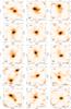 |
Fig. A.1 Line-free continuum emission at 345 GHz with ALMA 7 m array. Contours start at 7 × the rms noise and increase in a logarithmic scale. Red crosses mark the continuum sources with labels in white (see Table A.1). The beam is shown in the lower left corner of each panel. |
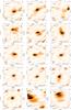 |
Fig. A.1 continued. |
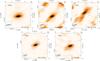 |
Fig. A.1 continued. |
Summary of physical properties of the sample.
All Tables
All Figures
|
Fig. 1 Left: Clump-scale view by ATLASGAL of an example source. Right: Line-free continuum emission at 345 GHz by the ALMA 7 m array. Contours start at 7σrms noise and increase in a logarithmic scale. White crosses indicate the extracted sources (see Table A.1). The synthesized beam is shown in the lower left corner. |
| In the text | |
|
Fig. 2 Mass distribution of MDCs within d ≤ 4.5 kpc. The Poisson error of each bin is shown as a grey line above the 10σrms completeness limit of 50 M⊙, the power-law fit is shown in a solid black line. Hashed area shows the distribution of the brightest cores ( |
| In the text | |
|
Fig. 3 Surface density vs. mass diagram. Coloured dotted lines in different shades show constant radius (green) and nH number density (red; cf. Tan et al. 2014). Coloured large circles show clumps (ATLASGAL), while smaller circles show the cores (ALMA 7 m array), colours scaling from blue to red with increasing |
| In the text | |
|
Fig. 4 Core formation efficiency vs. average clump density ( |
| In the text | |
|
Fig. A.1 Line-free continuum emission at 345 GHz with ALMA 7 m array. Contours start at 7 × the rms noise and increase in a logarithmic scale. Red crosses mark the continuum sources with labels in white (see Table A.1). The beam is shown in the lower left corner of each panel. |
| In the text | |
|
Fig. A.1 continued. |
| In the text | |
|
Fig. A.1 continued. |
| In the text | |
Current usage metrics show cumulative count of Article Views (full-text article views including HTML views, PDF and ePub downloads, according to the available data) and Abstracts Views on Vision4Press platform.
Data correspond to usage on the plateform after 2015. The current usage metrics is available 48-96 hours after online publication and is updated daily on week days.
Initial download of the metrics may take a while.