| Issue |
A&A
Volume 600, April 2017
|
|
|---|---|---|
| Article Number | A66 | |
| Number of page(s) | 20 | |
| Section | Stellar structure and evolution | |
| DOI | https://doi.org/10.1051/0004-6361/201629701 | |
| Published online | 31 March 2017 | |
RAVE stars in K2
I. Improving RAVE red giants spectroscopy using asteroseismology from K2 Campaign 1⋆
1 Leibniz-Institut für Astrophysik Potsdam (AIP), An der Sternwarte 16, 14482 Potsdam, Germany
e-mail: This email address is being protected from spambots. You need JavaScript enabled to view it.
2 School of Physics and Astronomy, University of Birmingham, Edgbaston, Birmingham, B15 2TT, UK
3 Stellar Astrophysics Centre, Department of Physics and Astronomy, Aarhus University, 8000 Aarhus C, Denmark
4 LESIA, Observatoire de Paris, PSL Research University, CNRS, Université Pierre et Marie Curie, Université Paris Diderot, 92195 Meudon, France
5 Osservatorio Astronomico di Padova, INAF, Vicolo dell’Osservatorio 5, 35122 Padova, Italy
6 Dipartimento Fisica e Astronomia, Universitá di Padova, 35122 Padova, Italy
7 Astronomisches Rechen-Institut, Zentrum für Astronomie der Universität Heidelberg, Mönchhofstr. 12−14, 69120 Heidelberg, Germany
8 Sydney Institute for Astronomy, School of Physics, University of Sydney, NSW 2006, Australia
9 Osservatorio Astronomico di Padova, INAF, 36012 Asiago (VI), Italy
10 Observatoire astronomique de Strasbourg, Université de Strasbourg, CNRS, UMR 7550, 11 rue de l’Université, 67000 Strasbourg, France
11 Research School for Astronomy and Astrophysics, Mount Stromlo Observatory, The Australian National University, ACT 2611, Australia
12 E. A. Milne Centre for Astrophysics, University of Hull, Hull, HU6 7RX, UK
13 Institute of Astronomy Cambridge University, Madingley Road Cambridge CB3 0HA, UK
14 Kapteyn Astronomical Institute, University of Groningen, PO Box 800, 9700 AV Groningen, The Netherlands
15 Lund Observatory, Box 43, 221 00 Lund, Sweden
16 Senior CIFAR Fellow, Dept. of Physics and Astronomy, University of Victoria, Victoria, BC, V8P 5C2, Canada
17 Department of Physics, The University of Hong Kong, Hong Kong, PR China
18 Department of Physics and Astronomy, Macquarie University, Sydney, NSW 2109, Australia
19 Centre for Astronomy, Astrophysics and Astrophotonics, Macquarie University, Sydney, NSW 2109, Australia
20 Mullard Space Science Laboratory, University College London, Holmbury St Mary, Dorking, RH5 6NT, UK
21 Sydney Institute for Astronomy, School of Physics, University of Sydney, NSW 2006, Australia
22 Australian Astronomical Observatory, PO Box 915, North Ryde, NSW 1670, Australia
23 Department of Physics and Astronomy, Johns Hopkins University, 3400 N. Charles St, Baltimore, MD 21218, USA
24 Faculty of Mathematics and Physics, University of Ljubljana, 1000 Ljubljana, Slovenia
Received: 12 September 2016
Accepted: 15 December 2016
Abstract
We present a set of 87 RAVE stars with detected solar like oscillations, observed during Campaign 1 of the K2 mission (RAVE K2-C1 sample). This data set provides a useful benchmark for testing the gravities provided in RAVE data release 4 (DR4), and is key for the calibration of the RAVE data release 5 (DR5). The RAVE survey collected medium-resolution spectra (R = 7500) centred in the Ca II triplet(8600 Å) wavelength interval, which although being very useful for determining radial velocity and metallicity, even at low S/N, is known be affected by a log (g)-Teff degeneracy. This degeneracy is the cause of the large spread in the RAVE DR4 gravities for giants. The understanding of the trends and offsets that affects RAVE atmospheric parameters, and in particular log (g), is a crucial step in obtaining not only improved abundance measurements, but also improved distances and ages. In the present work, we use two different pipelines, GAUFRE and Sp_Ace, to determine atmospheric parameters and abundances by fixing log (g) to the seismic one. Our strategy ensures highly consistent values among all stellar parameters, leading to more accurate chemical abundances. A comparison of the chemical abundances obtained here with and without the use of seismic log (g) information has shown that an underestimated (overestimated) gravity leads to an underestimated (overestimated) elemental abundance (e.g. [Mg/H] is underestimated by ~0.25 dex when the gravity is underestimated by 0.5 dex). We then perform a comparison between the seismic gravities and the spectroscopic gravities presented in the RAVE DR4 catalogue, extracting a calibration for log (g) of RAVE giants in the colour interval 0.50 < (J−KS) < 0.85. Finally, we show a comparison of the distances, temperatures, extinctions (and ages) derived here for our RAVE K2-C1 sample with those derived in RAVE DR4 and DR5. DR5 performs better than DR4 thanks to the seismic calibration, although discrepancies can still be important for objects for which the difference between DR4/DR5 and seismic gravities differ by more than ~0.5 dex. The method illustrated in this work will be used for analysing RAVE targets present in the other K2 campaigns, in the framework of Galactic Archaeology investigations.
Key words: stars: late-type / stars: oscillations / stars: abundances / stars: fundamental parameters / techniques: spectroscopic / surveys
Data (atmospheric parameters, abundances, distances, ages and reddening) are only available at the CDS via anonymous ftp to cdsarc.u-strasbg.fr (130.79.128.5) or via http://cdsarc.u-strasbg.fr/viz-bin/qcat?J/A+A/600/A66
© ESO, 2017
1. Introduction
Galactic spectroscopic surveys play a key role in modern astrophysics. They provide large data sets of stellar atmospheric parameters, velocities, distances and abundances, making it possible to test modern models of Galactic dynamical and chemical evolution. RAVE (Steinmetz et al. 2006), the Gaia-ESO survey (GES; Gilmore et al. 2012; Randich et al. 2013), GALAH (De Silva et al. 2015), APOGEE (Majewski et al. 2017), SEGUE (Yanny et al. 2009) and LEGUE (Zhao et al. 2012) are providing stellar catalogues of several hundred thousand objects.
Red giant stars are among the primary targets of spectroscopic Galactic surveys, since they are intrinsically bright and common objects and they can be observed in several components of the Milky Way. In addition, they cover a wide range in age, making it possible to reconstruct the history of our Galaxy. However, the measurement of stellar atmospheric parameters (effective temperature, Teff, and surface gravity, log (g)) of red giants via spectroscopic analysis is affected by known systematics (Morel & Miglio 2012; Heiter et al. 2015).
In this work, we focus on the log (g) determination. It is a well-known problem in the literature that the log (g) for late-type stars suffers from systematic systematic error of the order of 0.2 dex (Morel & Miglio 2012; Heiter et al. 2015; Takeda & Tajitsu 2015; Takeda et al. 2016). The causes of this systematic error are numerous, and are not only the use of a range of different techniques by different authors (e.g. ionization balance and line profile fitting). Among the culprits there are also the adoption of inaccurate line parameters (such as oscillator strength), the assumption of local thermodynamical equilibrium (LTE) and 1-D conditions, degeneracies and noisy or ill continuum-normalised spectra. As a consequence, an inaccurate measure of the gravity can lead to inaccurate estimates of Teff, chemical abundances, distances and stellar age since the determinations of these quantities are linked to and ultimately dependent on the log (g) estimate.
With the advent of asteroseismology and thanks to the valuable observations performed using the CoRoT (Baglin et al. 2006) and Kepler (Borucki et al. 2010) satellites, it has been possible to derive with high precision fundamental properties of red giant stars such as mass (M) and radius (R) by using their global seismic properties Δν (frequency separation) and νmax (frequency of maximum oscillation power). It was immediately realised that asteroseismology could have a large impact on galactic populations studies (Miglio et al. 2009, 2013).
The surface gravity determined from stellar oscillations proved to be more precise and accurate than that derived using only spectroscopy (Morel & Miglio 2012; Hekker et al. 2013; Heiter et al. 2015). This seismic log (g), log (g)seismo, can therefore be used as a powerful tool for testing the adopted spectroscopic pipelines and, eventually, calibrating them. In recent years, pipelines that derive atmospheric parameters and abundances implementing the seismic gravity have also been developed as GAUFRE (Valentini et al. 2013). Current spectroscopic surveys are largely taking advantage of the asteroseismic techniques, by including red giants for which asteroseismology is available, in their target list. CoRoT targets are now being observed by GES as calibrators (Pancino et al. 2016), Kepler targets have been used for calibrating stellar surface gravities in APOGEE (Pinsonneault et al. 2014) and LAMOST (Wang et al. 2016). The first results impacting Galactic archeology using asteroseismology coupled with spectroscopy are now starting to appear (Chiappini et al. 2015; Martig et al. 2015; Anders et al. 2017b,a; Valentini et al., in prep.).
The Kepler K2 mission (started on June 2014, Howell et al. 2014) is the continuation of the successful Kepler space mission. In 2014, the failure of two reaction wheels rendered observation of the original field no longer feasible. For this reason, a new mission, K2, was conceived, planning 80-day observational runs of a set of 14 fields located along the ecliptic plane. K2 is able to detect solar-like oscillations in field red giants (Stello et al. 2015) and clusters (Miglio et al. 2016), and the light curves were of sufficient quality for measuring seismic parameters. The satellite is now observing several hundreds of RAVE targets, making it now also possible to obtain asteroseismic information for RAVE red giants (Kepler, whose field was in the north hemisphere, has no common target with RAVE, and the few RAVE targets in common with CoRoT have overly noisy light curves).
The RAVE survey, completed in 2013, is the precursor of larger spectroscopic surveys. It provided an unprecedented view of our Galaxy, observing approximately 500 000 targets in the southern hemisphere. The DR4 catalogue (Kordopatis et al. 2013), provides stellar velocities and atmospheric parameters plus metallicities, with special attention devoted to the derivation of reliable metallicities using calibration data sets. The database also contains seven element abundances (Mg, Al, Si, Ca, Ti, Fe and Ni), derived using a dedicated abundance pipeline (Boeche et al. 2013). The estimated errors in abundance, based on a comparison with reference stars, depend on the element and signal to noise ratio (S/N). For S/N> 40 they range from 0.17 dex for Mg, Al and Si to 0.3 dex for Ti and Ni. The error for Fe is estimated as 0.23 dex. DR4 also provides distances, that were derived by using two different methods: via isochrone fitting (Zwitter et al. 2010) and via Bayesian distance-finding with kinematic corrections (Binney et al. 2014). The later method also gives an estimate of the stellar ages, albeit with large uncertainties (see Binney et al. 2014, for a discussion).
The log (g) determination is a problematic step for RAVE: its spectral interval suffers from a strong log (g)-Teff degeneracy, that causes an inaccurate log (g) measure for red giants and an offset, that causes the misplacement of the red clump by ~0.3 dex (Kordopatis et al. 2011, 2013; Binney et al. 2014). The main aim of this paper, the first in a series (where we use K2 targets in common with RAVE for galactic archaeology purposes) is to show the impact of using the precise and accurate seismic gravity in the outcome temperatures and abundances of RAVE targets. We also show how the approach discussed here helps improving the RAVE stellar parameters and abundances. As shown in Bruntt et al. (2012), Thygesen et al. (2012) and Morel et al. (2014) asteroseismology can play an important role in this respect, as it provides precise and accurate gravities, once more helping to break remaining degeneracies. Additional improvements regarding the lifting of the degeneracy are shown in DR5 Kunder et al. (2017), by using the new APASS photometric information, the infra-red flux method, and the log (g) calibration presented in this work.
The paper is organised as follows: in Sect. 2, we present the RAVE targets that have been observed in K2 Campaign 1; in Sect. 3, we present the seismic data available for our sample; in Sect. 4, we describe our spectroscopic analysis strategy in order to obtain highly consistent stellar parameters and therefore accurate stellar abundances for our sample. In Sect. 5, we compared our results with those of RAVE DR4 for the same stars, providing a calibration for the log (g)RAVEDR4. Section 6 focuses on demonstrating how variations in log (g) impacts element abundances, and what constitutes the safe parameter space over which our calibration can be applied. Distances and reddening (and ages), determined via a Bayesian approach using asteroseismology and the newly determined atmospheric parameters are shown in Sect. 7. In this section we also provide a comparison with the values obtained in DR4 and DR5 for the same stars. In particular, DR5 has made use of the seismic analysis presented in this work. In Sect. 8, we summarise our results.
2. RAVE targets in K2 Campaign 1
The K2 Campaign 1 has a field of view of 100 deg2, centred at RA 11h35m46s DEC +01°25′02′′ (l = 265, b = + 58), and is thus a field almost perpendicular with respect to the Galactic plane.
In the field of view of K2 Campaign 1 there are 1400 RAVE targets; among those, 247 are present in the K2-C1 target list (see Fig. 1). Seismic parameters Δν and νmax have been measured for 87 objects (see Sect. 3 for details). The S/N, Teff, log (g) and [M/H] distributions are shown in Figs. 2 and 3 (red histogram), while the log (g)-Teffdiagram of the targets, constructed using DR4 data, is shown in the left panel of Fig. 4. As visible in the last panel of Fig. 3, the metallicity distribution, computed using asteroseismology (filled blue histogram), tends to be more metal-rich than the RAVE DR4 one (red empty histogram), but it covers a large metallicity interval.
2.1. Spectra
RAVE spectra were taken using the 6dF facility, a multi-fibre spectrograph mounted at the 1.2-m UK Schmidt Telescope of the Australian Astronomical Observatory (AAO). Spectra cover a wavelength range of ~400 Å, from 8410 Å to 8795 Å. RAVE resolution is R = Δλ/λ = 7500. This wavelength range is widely used in the field of Galactic Archaeology: the presence of the strong Ca II triplet (λ = 8498.02 Å, 8542.09 Å, 8662.14 Å) makes it possible to measure radial velocity (RV) even at low S/N. The Ca II triplet also acts as metallicity indicator (e.g. Da Costa & Hatzidimitriou 1998). Using several features of Fe and α-elements (Mg, Si, Ca, Ti), it is also possible to measure element abundances, as shown in Boeche et al. (2013), Kordopatis et al. (2013) and Boeche et al. (2014). The same wavelength interval is covered by Gaia-ESO survey (HR21 set-up of the FLAMES-GIRAFFE multi-object spectrograph) and the Gaia Radial Velocity Spectrometer (Gaia-RVS).
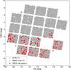 |
Fig. 1 RA-Dec position of the targets observed by K2 during Campaign 1 (grey dots); the field is centred at 11:35:46 +01:25:02 and it was observed from 30-05-2014 to 21-08-2014. Empty red circles mark the RAVE stars observed by K2, while full red circles mark the 87 RAVE targets with detected oscillations. |
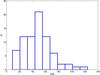 |
Fig. 2 S/N distribution of the spectra of the 87 RAVE stars possessing asteroseismology. |
2.2. Photometry
RAVE DR4 catalogue contains DENIS DR3 (DENIS Consortium 2005) and 2MASS (Cutri et al. 2003) photometry. In this work, the photometry of DR4 is implemented with the APASS photometry for RAVE targets from Munari et al. (2014). APASS provided photometry in the Landolt BV and Sloan g′r′i′ bands. APASS photometry is available for all the 87 targets of our RAVE-K2 sample in Campaign 1. We also added the WISE W1 and W2 filters photometry from the AllWISE catalogue (Cutri et al. 2013).
The Munari et al. (2014) catalogue also provides photometric temperatures computed in 6 different ways. For our analysis, we focused on the Teff derived by simultaneously fitting EB−V, in order to avoid systematics introduced by the adoption of a fixed value for distance, reddening, log (g) or [M/H].
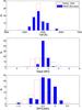 |
Fig. 3 Distribution of Teff, log (g) and [M/H] of the RAVE stars analysed in this work. RAVE DR4 values are plotted in empty, red bars; the new atmospheric parameters derived using asteroseismology are plotted with blue, filled bars. |
3. Asteroseismic data
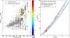 |
Fig. 4 Left panel: log (g)-Teff distribution of RAVE targets in K2-C1 target list (grey dots). Atmospheric parameters and errors are taken from RAVE DR4. Targets possessing Δν and νmax are colour-enhanced (by following calibrated [M/H] from RAVE DR4 catalogue) and circled in black. The dashed lines in log (g) mark the K2 detection limits at 2.1 and 3.35 dex. Right panel: Δν and νmax distribution of the 87 RAVE targets in K2-C1 possessing seismic parameters. The distribution is superimposed onto three Δν -νmax distributions calculated following Padova isochrones, taken at three different metallicities and ages. |
The Campaign 1 field was observed by K2 from May 30, 2014 to August 21, 2014. The satellite observed 21 647 targets in the field.
RAVE targets analysed in this work were observed as part of the “The K2 Galactic Archaeology Program Campaign 1” (C1 proposal GO1059, Stello et al. 2015). The target list of this project was composed of red giants belonging to some of the most important spectroscopic surveys, such as RAVE, APOGEE and GALAH.
Pixel masks for the individual C1 targets were defined using the K2P2 pipeline (K2-Pixel-Photometry; Lund et al. 2015). First a summed image (over time) is constructed that includes the apparent motion of the stars on the CCD due to the characteristic 6-h drift of the spacecraft (Howell et al. 2014; Van Cleve et al. 2016). A set of unsupervised machine learning techniques are applied in K2P2 to the summed image to define the pixel masks from which raw light curves are extracted. Instrumental features in the raw-flux light curves are corrected for using the strong correlation of these with the stellar position on the CCD. Finally, the light curves are corrected for further artefacts using the KASOC filter (Handberg & Lund 2014) with adopted time scales of τlong = 3 days and τshort = 0.25 days for the median filters (we refer to Handberg & Lund 2014, for additional information on the KASOC filter).
To estimate the frequency of maximum oscillation power, we adopted the technique described in Davies & Miglio (2016) based on fitting a background model to the data. We fitted model H of Kallinger et al. (2014), comprised of two Harvey profiles, a Gaussian oscillation envelope and an instrumental noise background. For the estimate of νmax we took the central frequency of the Gaussian component. We used the median and the standard deviation to summarise the normal-like posterior probability density for νmax. The latter parameter has been measured for 87 RAVE stars. As an external check, νmax has also been estimated using the technique of Mosser et al. (2011): the νmax values measured by the two independent techniques agree very well, with a median fractional difference below 1%.
To estimate the average frequency separation, we adopted the method described in Mosser & Appourchaux (2009) and Mosser et al. (2011). This method uses the expected frequency pattern of a red giant for identifying oscillation modes. Δν was then measured for 86 RAVE stars. We performed a reliability check of the seismic parameters by using the PARSEC set of isochrones (Bressan et al. 2012) following the approach adopted by Valentini et al. (GES in prep.). We considered three isochrones,at [ Fe / H ]=−1.0, 0.0 and +0.5 dex and of age 10, 5 and 1 Gyr, respectively. All the 86 stars possessing both Δν and νmax fall within the predicted distribution.
In this work we therefore adopted the νmax and its uncertainty for 87 stars, measured using the Davies & Miglio (2016) technique. Of those stars with detected νmax, 86 possess Δν values measured using the (Mosser et al. 2011) method (with their uncertainties).
4. Spectroscopic analysis
Input physics of GAUFRE and Sp_Ace codes.
As widely discussed in Kordopatis et al. (2011, 2013), the wavelength interval observed by RAVE suffers from a strong degeneracy between effective temperature and surface gravity, because of the low resolution (R ≤ 10 000) combined with the small wavelength coverage. The wavelength interval possesses too few spectral features sensitive to Teff or log (g) only; often the same feature is used as a Teff and log (g) indicator at the same time. This leads to degeneracies, due to the fact that a spectral line can have the same depth and shape for two stars with different atmospheric parameters. One solution might be to identify additional spectral features sensitive to one parameter only, to change the algorithm in the pipeline (overcoming the classical χ2 minimization technique) or to use external information that already provides an indication of the temperature and gravity of the object.
In the work of RAVE DR4, the log (g)-Teff degeneracy was partially solved by adopting a combination of a decision-tree algorithm and a projection method (method explained in Kordopatis et al. 2011), with an approximate initial Teff selection based on photometric temperatures.
In this work, we show that when seismic information is available, the determination of reliable atmospheric parameters and abundances is also possible for algorithms that use the distance minimisation. The main problem with pipelines that adopt the minimum distance method, is that the degeneracies wipe out the identification of the minimum. For example, the pipeline risks converging at a secondary minimum, or two very close secondary minimums can merge, leading to an incorrect or imprecise solution. Asteroseismology, combined with photometry and spectroscopy, avoids this problem: the log (g) is fixed to the seismic value and the temperature provided by photometry is used as prior, removing the degeneracy of the spectroscopic analysis, and reducing the risk of convergence into secondary minima.
For the spectroscopic analysis of the RAVE spectra, we used two pipelines: GAUFRE, for the log (g) and Teff determination, and Sp_Ace for the determination of overall metallicity and abundances. Sp_Ace had already been successfully used in previous tests for deriving stellar parameters and element abundances and performs well at low resolutions. GAUFRE works using seismic values in order to iteratively derive log (g), Teff and [ Fe / H ] . We decided on the adoption of two pipelines because, at the moment, Sp_Ace does not allow the adoption of probabilistic priors, but takes fixed Teff and log (g) as input. The two pipelines are described in the following Sect. 4.1.
4.1. Description of the adopted spectroscopic pipelines
GAUFRE: GAUFRE (Valentini et al. 2013) is a spectroscopic pipeline that implements asteroseismology in the derivation of atmospheric parameters, and is currently used in the analysis of CoRoT-GES targets, Valentini et al. (GES in prep.).
It is a C++ collection of several routines, designed for the spectroscopic analysis of high-resolution spectra of F-G-K giants in the optical domain. For the analysis of the RAVE spectra we used the GAUFRE-SISMO and the GAUFRE-CHI2 routines to iteratively derive atmospheric parameters via χ2 fitting on a library of synthetic spectra by fixing the gravity to the seismic one. The spectral library used in this work, is the one provided by L. Fossati and degraded to the RAVE resolution of R = 7500, covering the 8350−8850 Å spectral range. The synthetic spectra has been computed using Synth3 code (Kochukhov 2007, 2012) and using Castelli & Kurucz (2004) model atmospheres and VALD3 linelist. Synthetic spectra were renormalised using the same function as most of the RAVE spectra: an order 4 cubic spline with 1.5σ and 3.0σ low- and high-level rejection thresholds (Zwitter et al. 2008; Siebert et al. 2011). For our analysis we masked the cores of the strong CaII triplet lines (that may be affected by NLTE effects, see Jorgensen et al. 1992).
In this work the GAUFRE pipeline has been used for iteratively deriving Teff and log (g), by using APASS photometric temperatures as a prior (providing a flexibility of ±500 K) and fixing the gravity to the seismic one. The validation of this method is discussed in Sect. 4.2. The input physics of the two codes is summarised in Table 1.
Sp_Ace: SP_Ace is a FORTRAN95 code that can estimate Teff, log (g) and elemental abundances from normalized radial-velocity-corrected stellar spectra. It derives the parameters seeking the minimum χ2 computed from the observed spectrum and model spectra, the latter constructed by SP_Ace from a library of General Curves-Of-Growth (GCOG, see Boeche & Grebel 2016, for details). As shown in Boeche & Grebel (2016), SP_Ace performs well between spectra resolutions 2000 and 20 000, which include the RAVE resolution. Among other features, this code allows the user to determine the chemical abundances by fixing log (g) and/or Teff to trusted values. In this work we run SP_Ace by adopting the options “ABD_loop” (which rules the SP_Ace internal iterations between the routines that estimates the stellar parameters Teff and log (g) and the abundances) and “norm_rad = 10” (which rules the re-normalisation of the observed spectrum).
We used the Sp_Ace pipeline for determining metallicity and abundances, by fixing the Teff and log (g) to the values derived iteratively by GAUFRE. The validation of this method is discussed in Sect. 4.2.
4.2. Pipelines validation
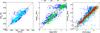 |
Fig. 5 Comparison of the atmospheric parameters (from left to right: Teff, log (g) and [ Fe / H ] ) of the calibration set versus the values derived using the GAUFRE pipeline. Parameters were derived adopting four different strategies, following the same code as Fig. 7. Mean dispersions and offsets are displayed in Table 2. |
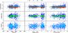 |
Fig. 6 Comparison of the atmospheric parameters (from top to bottom: [ Fe / H ] , log (g) and Teff) measured by the GAUFRE pipeline, versus the atmospheric parameters available in the literature. Different symbols mark different approaches, following the same code as Fig. 7. Mean dispersions and offsets are displayed in Table 2. |
For the validation of the two pipelines, we derived atmospheric parameters and abundances for the set of reference stars used in RAVE DR4 (Kordopatis et al. 2013). The RAVE DR4 calibration data sets of observed spectra consist of 809 spectra of giants and dwarfs belonging to the field or open clusters. All the spectra have a signal-to-noise ratio (S/N) > 40 pixel-1. The sample was constructed in order to cover as much as possible the parameter space of the stars observed by the RAVE survey. The RAVE reference catalogue comprises heterogeneous sources: a set of 169 RAVE giants and dwarfs with multiple PASTEL entries (Soubiran et al. 2010), 224 dwarfs and giants present in the CFLIB library (Valdes et al. 2004), 163 giants observed by Fulbright et al. (in prep.), 229 spectra of giants and dwarfs from Ruchti et al. (2011), 22 spectra of stars belonging to M67 and IC 4651 open clusters (Pancino et al. 2010; Pasquini et al. 2004) and two spectra of the metal poor ([ Fe / H ] = −4.2) giant CD-38245 (Cayrel et al. 2004). For details regarding the construction and the computation of the atmospheric parameters of the RAVE calibration data sets, we refer to Kordopatis et al. (2013).
In order to simulate what happens using asteroseismology and when fixing different parameters, we run the two pipelines on the calibration set in four different ways:
-
no constraints in log (g) nor Teff (coded as-NP);
-
Teff fixed (coded as -TP);
-
log (g) fixed (coded as -GP);
-
fixed Teff and log (g) (coded as -TGP).
Due to the limits of both pipelines, we considered only those targets with [ Fe / H ]>−2.5 dex. The comparisons of the reference literature values with those derived by the two pipelines are shown in Figs. 7 and 5 for Teff, log (g) and [ Fe / H ] . Offsets and dispersions of each pipeline for all four runs, are shown in Tables 3 and 2. Possible trends and offsets have been investigated in Figs. 8 and 6, for the SP_Ace and GAUFRE pipelines, respectively. In the red giant regime of the -NP analysis, the two pipelines show an offset in log (g) and a large spread, plus a trend that also persists when fixing the temperature to the literature value. A direct comparison between the SP_Ace and GAUFRE pipeline is illustrated in Figs. 9 and 10, while offsets and dispersions are reported in Table 4. These offsets, dispersions and trends are the result of the short wavelength coverage of the survey: in the 400 Å of the spectrum there are insufficient identified features able to solve the log (g)-Teff degeneracy.
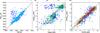 |
Fig. 7 Comparison of the atmospheric parameters (from left to right: Teff, log (g) and [ Fe / H ] ) of the calibration set versus the values derived by using SP_Ace pipeline. Parameters were derived adopting four different strategies: with no prior (blue triangles), fixing the temperature to the real value (green squares), fixing the gravity (cyan stars) and fixing temperature and gravity (red circles). Mean dispersions and offsets are displayed in Table 3. |
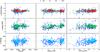 |
Fig. 8 Comparison of the atmospheric parameters (from top to bottom: [ Fe / H ] , log (g) and Teff) measured by the SP_Ace pipeline, versus the atmospheric parameters available in literature. Different symbols mark different strategies adopted for the analysis, following the same code as in Fig. 7. Mean dispersions and offsets are displayed in Table 3. |
When the information on log (g) and Teff are available, however, the two pipelines are capable of determining a value for metallicity that is in good agreement with the literature. The GAUFRE pipeline shows an offset in [ Fe / H ] of ~−0.10 dex, due to the presence of a strong feature in the synthetic spectra that are not present (or that are less strong) in the real spectra. This metallicity shift does not depend on any other atmospheric parameter and can be corrected by adding +0.1 dex to the [ Fe / H ] value given by the pipeline, or by upgrading the linelist, correcting the line parameters of the problematic features. For this work we used only the log (g) and Teff determined by GAUFRE, and computed the overall metallicity and abundances using SP_Ace . When fixing the log (g) and Teff to the literature values, SP_Ace shows no offset in metallicity (−0.01 dex for giant stars). Such hybrid use of results does not introduce internal inconsistencies.
Mean dispersions and offsets for Teff, log (g) and [ Fe / H ] of the GAUFRE pipeline with respect to the literature values for the calibration data set.
Mean dispersions and offsets for Teff, log (g) and [ Fe / H ] of the SPACE pipeline with respect to the literature values for the calibration data set.
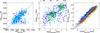 |
Fig. 9 Comparison of the atmospheric parameters (from left to right: Teff, log (g) and [ Fe / H ] ) of the calibration set atmospheric parameters as measured by GAUFRE versus the values derived with the SP_Ace pipeline. Parameters were derived adopting four different strategies: with no prior (blue triangles), fixing the temperature to the real value (green squares), fixing the gravity (cyan stars) and fixing temperature and gravity (red circles). Mean dispersions and offsets are displayed in Table 4. |
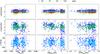 |
Fig. 10 Comparison of the atmospheric parameters (from top to bottom: [ Fe / H ] , log (g) and Teff) measured by the SP_Ace pipeline, versus the atmospheric parameters measured by GAUFRE. Different symbols mark different strategies adopted for the analysis, following the same code as in Fig. 9. Mean dispersions and offsets are displayed in Table 4. |
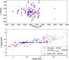 |
Fig. 11 Top panel: comparison between the Teff derived in this work, with and without asteroseismology (blue points and blue triangles respectively) and in RAVE DR4 (red points) versus the one obtained using APASS photometry (Munari et al. 2014). Bottom panel: comparison between the log (g) derived in this work, with and without asteroseismology (blue points and blue triangles, respectively) and in RAVE DR4 (red points) versus the one obtained using APASS photometry (Munari et al. 2014). |
Mean dispersions and offsets for Teff, log (g) and [ Fe / H ] of the GAUFRE pipeline with respect to the values measured by SP_Ace for the calibration data set.
4.3. Atmospheric parameters and abundances determination
For our analysis we considered the Teff and log (g)seismo derived using GAUFRE, adopting photometric Teff as a prior and with the gravity fixed to the seismic log (g). We then adopted the [ Fe / H ] and individual element abundances derived by SP_Ace, by fixing the Teff and log (g) provided by GAUFRE. This strategy is needed since GAUFRE allows the iterative determination of the atmospheric parameters by using the photometric temperature as a prior (within a 600 K interval), while Sp_Ace can take a fixed value of Teff and log (g), and provides chemical abundances estimation.
We determined the seismic log (g) using the νmax, the frequency corresponding to the maximum oscillation power. Starting from the scaling relation that links νmax to the stellar mass and radius (Brown et al. 1991; Kallinger et al. 2010; Belkacem et al. 2011): 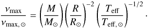 (1)It is possible to obtain a direct formula for the log (g) (by using the fundamental relation g = GM/R2, where G is the Newtonian gravity constant, M is the stellar mass and R is the stellar radius):
 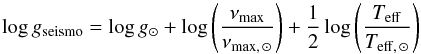 (2)with νmax ⊙ = 3140.0 μHz (Pinsonneault et al. 2014), Teff ⊙ = 5777 K and log (g)⊙ = 4.44 dex.
This equation for the surface gravity is weakly sensitive to the effective temperature and, following that νmax can be well determined, it can provide log (g) with a precision better than 0.03 dex (Kallinger et al. 2010; Morel & Miglio 2012). For a discussion on the accuracy of the relation in Eq. (2) see a discussion in Davies & Miglio (2016). Since the pipelines adopted in DR4 cannot work by fixing the log(g) to the seismic value, we performed our iterative analysis by using GAUFRE and Sp_Ace.
Thanks to the tests discussed in Sect. 4.2, we determined the atmospheric parameters using the following strategy:
-
1.
determination of the log (g)seismo adopting the APASS photometric temperature, using Eq. (2);
-
2.
analysis with GAUFRE by fixing the log (g) to the seismic value and using TeffAPASS as prior (Teff value can vary within a range of 500 K);
-
3.
analysis with GAUFRE fixing the gravity to the log (g)seismo determined using the Teff measured at step 2;
-
4.
run GAUFRE iteratively until convergence (usually three iterations are needed);
-
5.
Run Sp_Ace by fixing log (g) and Teff to the values determined by GAUFRE for determining abundances.
The top panel of Fig. 11 shows a comparison between the Munari et al. (2014) photometric Teff with the temperatures derived in this work (with and without using asteroseismology) and those present in RAVE DR4. As the temperature increases, the dispersion of the difference in Teff increases. This behaviour is partially due to the increase of the differences in the reddening determination (hotter stars are intrinsically brighter and hence more distant than the colder stars at the same apparent magnitude). The bottom panel of Fig. 11 shows the difference of the log (g) determined with different approaches (GAUFRE with no seismo, DR4 and GAUFRE with seismo) with respect to the log (g) computed using asteroseismology and the APASS photometric temperature. The strong degeneracy affecting the spectra causes the trend visible in the gravities determined from the pure spectroscopic analysis: the two pipelines show the same behaviour, even if using different approaches.
Internal errors in atmospheric parameters and abundances in RAVE DR4 and those computed by combining spectroscopy and asteroseismology.
The method adopted in this work converged for 72 stars of the 87 analysed. The non-convergence of the pipelines was due to: a bad S/N (method not working for S/N< 15), emission lines or non-corrected cosmic rays in the spectrum and/or metallicity too close (or outside) to the pipeline’s limits. The latter is the case of the two metal-poor stars; those stars are not present in this work since their atmospheric parameters and abundances have been derived manually.
Table 5 reports the typical internal errors in atmospheric parameters and abundances reported in the RAVE DR4 catalogue and those derived in this work. The adoption of the seismic log (g) significantly improved the accuracy of the Teff and abundances measurement.
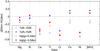 |
Fig. 12 Element variations when applying a variation to Teff and log (g) of ±150 K and ±0.50 dex. Differences between elements depend on the lines adopted and on the way their Curve of Growth (COG) depends on atmospheric parameters. |
4.4. Abundances measurement uncertainties
In order to understand the impact of strong offsets in temperature and metallicity to the element abundances determination, we re-derived the abundances of the benchmark stars using SP_Ace by assuming the following shifts in stellar parameters: ±150 K in Teff and ±0.5 dex in log (g).
As expected, an overestimation/underestimation of Teff and log (g) translates to an overestimation/underestimation of the element abundance. The derived abundances of different elements vary differently, following the way the COG of the individual lines responds to the variation of log (g) and Teff. Figure 12 shows how the different elements (plus [M/H]) vary with respect to the value obtained by assuming the correct Teff and log (g).
4.5. The RAVE spectra classification tool
The diagram in Fig. 14 shows the two-dimensional t-SNE (van der Maaten & Hinton 2008) projection of approximately 420 000 RAVE spectra with S/N> 10. Each spectrum was re-sampled to 768 common wavelength points and put into the data matrix that was used as an input to the t-SNE dimensionality reduction method. The projection shows groups with similar spectra together without requiring any assumptions about the stellar parameters. Naturally, spectra of giant stars being morphologically different from their dwarf counterparts are grouped in the different parts of the projection. In addition to the two main areas populated by the dwarfs and the giants, the manifold also includes peninsulas and islands occupied by less regular types such as spectroscopic binaries, hot stars, chromospherically active stars and so on. It is obvious from the figure that the majority of the stars from this study fall along the giant part of the manifold (log g< 3.5). There are two stars that fall onto the very metal-poor island (top right) and two that reside in the dwarf region. The latter have very low S/Ns and therefore their positioning in this diagram cannot be reliably used for confirmation of their gravity.
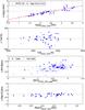 |
Fig. 13 Difference in log (g), Teff, [M/H] (calibrated and not calibrated) and [Mg/Fe] (Δ computed as RAVE DR4 − this work) for the 62 RAVE targets where the GAUFRE+Sp_Ace pipelines converged. In the top panel, the log (g) comparison, the fit used for calibrating log (g)RAVEDR4, is shown (red dashed line). |
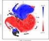 |
Fig. 14 t-SNE projection of approximately 420 000 RAVE spectra. The scaling in both directions is arbitrary, therefore the units on the axes are omitted. The colour-scale corresponds to the gravity of the stars as computed by Kordopatis et al. (2013). Giants are shown in red and dwarfs in blue. Lighter shaded hexagons include fewer stars than darker ones. Over-plotted black dots indicate locations of the stars from this study. |
5. Calibrating DR4 log g: towards an improved DR5
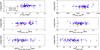 |
Fig. 15 Difference in log (g) (computed as log (g)RAVEDR4−log (g)seismo (empty circles) and log (g) |

RAVE red giants, and, in particular, red clump stars, have been widely used for investigating the properties of our Galaxy (e.g. Bilir et al. 2012; Williams et al. 2013; Bienaymé et al. 2014; Boeche et al. 2011). In these analyses giants and red clump stars were selected using photometric colour and a cut in log (g) (different approaches shown in Table 6). Since all the stars used fall in the 0.5 ≤ (J−KS) ≤ 0.8 and 1.8 ≤ log gRAVE ≤ 3.5 intervals, our sample of RAVE-K2 giants with asteroseismology is representative for understanding the offsets that can affect the RAVE red giants. In fact, RAVE-K2 red giants possess 0.5 ≤ (J−KS) ≤ 0.8 and 1.3 < log gRAVE< 4 dex.
As clearly visible in the top panel of Fig. 13, there is a trend affecting DR4 log (g): the latest RAVE pipeline tends to distribute red giants on a wide gravity interval, classifying some giants as dwarfs or supergiants. This misclassification, as visible in Fig. 15, does not depend on colour index, metallicity (calibrated or not-calibrated) or S/N. There is a trend of the log (g) depending on temperature, as one expects, since the two parameters are correlated.
Selection criteria adopted in different works for creating the sample of red giants or red clump stars.
Using the K2C1-RAVE sample, we obtained the following calibration for the RAVE DR4 gravities (plotted as a dashed line in the top panel of Fig. 13): 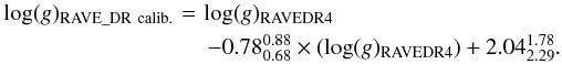 (3)For the fit we considered only RAVE DR4 stars where the algorithm successfully converged (“Algo_Conv_K” = 0 and “Algo_Conv_K” = 4, see Kordopatis et al. 2013, for the definition of these flags).
Since the difference in log (g) does not seem to depend on photometric colour, metallicity or S/N, the gravity calibration is only linearly dependent on the original log (g)RAVEDR4.
The temperatures and abundances can be re-computed in order to obtain more consistent values for the RAVE giants.
5.1. Sanity check: comparison with APOGEE and GES gravities
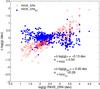 |
Fig. 16 Difference in log (g) (computed as log (g)RAVEDR4−log (g)APOGEE) vs. log (g)RAVEDR4 for the 855 RAVE targets in common with APOGEE-DR13. |
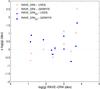 |
Fig. 17 Difference in log (g) (computed as log (g)RAVEDR4 – log (g)GES) vs. log (g)RAVEDR4 for the 11 RAVE targets in common with GES. Triangles represent stars observed by GES using UVES, circles those observed using GIRAFFE instrument. |
Since some RAVE red giants were observed by both APOGEE and GES surveys, we now compare gravities of these targets with those present in RAVE DR4, and the new log (g)s calibrated using Eq. (3).
APOGEE: There are 1422 targets in common between RAVE DR4 and APOGEE-DR13. Of those targets, 405 fulfill the quality criteria (convergence and quality flags for both RAVE and APOGEE) and lie in the colour interval 0.5 < (J−KS) < 0.8. A comparison between the log (g) is shown in Fig. 16. The log(g) provided by APOGEE was calculated by applying an a-posteriori calibration to the log (g) measured by the pipeline. This APOGEE calibration was based on the seismic gravities of RGB stars from Kepler data, as described in Holtzman et al. (2015). Since they used only the RGB stars for calibrating log (g), red clump gravities are overestimated by 0.2 dex. Figure 16 clearly shows that the calibration adopted here for the RAVE DR4 gravities (see Eq. (3)) leads to a good agreement with the APOGEE ones. Recently, Hawkins et al. (2016) recomputed abundances for the APOGEE Kepler stars by fixing the log (g) to the seismic gravity using the BACCHUS code, albeit without the iterative Teff-log (g) strategy adopted in this work.
GES: There are 142 targets in common between RAVE DR4 and GES-DR4. Of those targets, 11 fulfill the quality criteria (convergence and quality flags for both RAVE and GES). A comparison between the log (g) is shown in Fig. 17. GES provides homogenised atmospheric parameters and abundances, and in this work we considered F-G-K stars observed with UVES (high resolution, R = 47 000) and F-G-K stars observed with GIRAFFE (low resolution, R = ~ 19 000). The homogenisation is performed over the results provided by several pipelines (more than ten nodes involved), and weighted following the performances of the several nodes on a calibration set of stars (GES in prep.). The consistency within the different approaches used by each node is guaranteed by the fact that all the nodes use the same linelist (GES in prep.), the same set of model atmospheres (MARCS, Gustafsson et al. 2008) and the same library of synthetic spectra (de Laverny et al. 2012).
Although the number of red giants in common between the two surveys is not statistically meaningful, the trend is reduced when the correction of Eq. (3) is applied to RAVE log (g). In addition GES log (g) is the result of a homogenisation of different pipelines and is not calibrated using asteroseismology.
6. Impact of the adoption of the seismic log(g) on atmospheric parameters and abundances
At medium resolution, the CaII triplet region does not provide very much information regarding stellar gravity, and this problem is also present in RAVE DR4.
By comparing the seismic log (g) with those provided in DR4, a clear trend is visible (first panel of Fig. 13). In some cases, the RAVE DR4 pipeline tends to identify giants as hot dwarfs or cold supergiants. This misclassification is due to the log (g)-Teff degeneracies affecting the RAVE spectral interval.
6.1. Temperatures
Figure 18 shows a comparison of the temperature determined at the present work for our 72 RAVE-K2-C1 stars, with the values reported in DR4, DR5 and those of the IRFM as in DR5. A general agreement is found, except for the hotter stars.
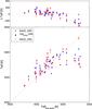 |
Fig. 18 Effective temperatures obtained in this work compared with those from the IRFM temperatures (blue dots), RAVE(DR4) (open circles) and RAVE(DR5) (red points). |
Indeed, it can be seen that at high temperatures (Teff> 5000 K), there is a discrepancy between the temperatures derived using log (g)seismo and those present in DR5, the spectroscopic ones, those derived using the IRFM (adopting the method described in Casagrande et al. 2006), and those in DR4. As expected, the most deviant stars correspond to those for which there is a larger difference in log (g) with respect to the seismic value (the top panel of Fig. 19). The discrepancy in Teff might be due to the log (g) discrepancy, since Casagrande et al. (2006) IRFM is slightly dependent on theoretical models, which for RAVE DR5 had been constructed using DR5 Teff, log (g) and [ Fe / H ] .
Thanks to the iterative process for deriving log (g) and Teff, we consider our temperatures reliable. The high precision of the log (g)seismo and the fact that it is weakly dependent on temperature, help in partially removing the degeneracy and in deriving an accurate temperature.
6.2. Abundances
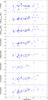 |
Fig. 19 Differences in Teff, [M/H] (not calibrated and calibrated), [ Fe / H ] , [Mg/H], [Ni/H], [Ti/H] and [Si/H] vs. the differences in log (g). All differences are defined as RAVE(DR4) − (this work). The vertical dashed lines mark the | Δlog (g) | = 0.5 dex limits. |
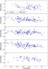 |
Fig. 20 Distributions of alpha-elements (Ni, Ti, Si, Al, Mg) plus Cr versus Fe of the RAVE stars analysed in this work. Filled blue dots are the abundances obtained by using asteroseismology, black circles are the original DR4 values. |
The abundance determination is linked to the determination of the atmospheric parameters. Since log (g) and Teff varied strongly from the spectroscopic determination of RAVE DR4 to the seismically determined one, we expect element abundances to vary as well.
Figure 19 illustrates how the element abundances of Fe, Mg, Ni, Ti and Si (in addition to overall metallicity and temperature) vary depending on the difference in log (g). As expected, in general, when the DR4 gravity is underestimated, the element abundance is underestimated, and when the gravity is overestimated, the abundances are overestimated as well. The same happens for overall metallicity, both calibrated and not calibrated. However, Fig. 19 also shows that for the objects where the discrepancy between the gravities measured here and those of DR4 remains within 0.5 dex, the chemical abundances are only slightly affected.
Since the DR4 metallicity is calibrated following a function depending on log (g) and [M/H], there is an additional risk to introducing some metal-rich and metal-poor red giants simply as a result of an erroneous log (g) determination in addition to an excessive metallicity correction.
The distributions of the α-elements (Mg, Si and Ti) do not vary significantly with respect to DR4, as seen in panels b, c and d of Fig. 20. The field is observing targets distributed perpendicularly to the Galactic plane (see Fig. 23), belonging to the thin and the thick disks. As one should expect for this field, Fe-poor objects are alpha-enhanced. Fe-peak elements (Ni and Cr, panels a and e of Fig. 20) do not vary following metallicity. Again, this trend follows what is expected, since Fe-peak elements are supposed to vary as Fe does.
6.3. DR5 calibration
The results presented in this paper have been used to calibrate two catalogues in RAVE DR5: a) the main DR5 catalogue, which adopts a calibration for all stars (dwarfs and giants), computed using seismic log (g)s from our 72 stars plus the Gaia benchmark stars; and b) the seismic calibrated catalogue of giants (DR5-SC) in the same colour range as the stars studied in this work, where the calibration adopted is the one presented in Eq. (3) (as in both the DR4 and DR5, the same spectroscopic pipeline is adopted). For the DR5-SC, the chemical abundances were computed with calibrated gravities and the IRFM temperatures (for a comparison of the CMD of the RAVE DR5 SC and RAVE DR5 catalogues, see Appendix).
Figure 21 shows the metallicity distribution of the DR5 seismic calibrated catalogue in comparison with the MDF obtained for the same stars, but with DR5 (main catalogue) metallicities. Although similar, the DR5-SC MDF is narrower and has less metal-rich stars than the DR5 or DR4 MDFs. We also checked the MDF of the DR5-SC catalogue upon the removal of stars with temperatures above 5000 K (for which the IRFM temperatures differ from the ones obtained in our analysis, see Fig. 18), but the MDF did not change.
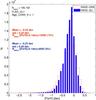 |
Fig. 21 Metallicity distribution of RAVE DR5 seismic calibrated giants (RAVE-SC, see Kunder et al. 2017), compared with the MDF for the same stars but with DR5 metallicities. |
7. Distances, reddening (and ages)
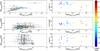 |
Fig. 22 Comparison of distances, reddening (AV) and age derived using PARAM versus RAVE DR4 data. Data are colour-coded following the difference in gravity. Differences for the various quantities are always computed as: Δ = RAVE DR4 − this work. Top left panel: distances derived by PARAM vs. distance in RAVE DR4 (computed as the inverse of the parallax). Top right panel: distance residuals (in %) vs. log (g)seismo. Left central panel: AV derived by PARAM vs. AV present in RAVE DR4 catalogue. Right central panel: AV residuals vs. log (g)seismo. Bottom right panel: ages derived by PARAM vs. RAVE DR4 ones. Bottom left panel: age residuals (in %) vs. log (g)seismo. |
For our analysis we used masses, radii, distances, reddening and ages derived using the PARAM1 tool (da Silva et al. 2006; Rodrigues et al. 2014) that derives stellar distance, reddening and age through Bayesian estimation. For this work, we used the Rodrigues et al. (2014) version, implemented with the possibility of using seismic information (Δν, νmax and evolutionary status). The code uses the seismic information by calculating Δν and νmaxfrom the Bressan et al. (2012) set of isochrones using the scaling relations: 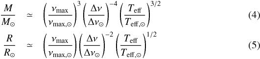 where νmax ⊙ = 3140.0 μHz, Δνmax ⊙ = 135.03 μHz (Pinsonneault et al. 2014), Teff ⊙ = 5777 K.
As input parameters we adopted the refined atmospheric parameters described in Sect. 4, the seismic Δν and νmax described in Sect. 3, and the photometric information from 2MASS, DENIS-I, AllWISE and APASS. PARAM converged for 67 stars (out of 72).
Figure 23 shows the spatial distribution, in Galactic radius (Rnow) and height to the Galactic plane (Z) of the stars. Stars are distributed perpendicularly to the Galactic plane, reaching a maximum Z of 1.5 kpc, with Rnow spanning from 7.9 to 8.3 kpc, and are thus representative of both the thick and thin disks.
Figure 22 shows the comparison between distances, reddening (and ages) derived by PARAM, with those provided in RAVE DR4, distance and reddening offset and dispersions are reported in Table 7. Since in this work we are not focusing on individual stellar ages and their individual errors, we consider the PARAM ages as a relative age indication, able to only discriminate old stars from intermediate and young objects.
Figure 24 is similar to Fig. 22, but shows the comparison with the DR5-SC values (results of the comparison with RAVE DR5 main catalogue are not shown, as the results are similar to the ones shown here).
In the distances comparison with RAVE DR4, we considered distances derived from parallaxes, as suggested by Binney et al. (2014). Red clump gravities in DR4 are overestimated by ~0.3 dex, leading to a distance overestimation of ~25%. The same problem can also happen with the rest of the red giants. The adoption of an imprecise log (g) and reddening, results in an overestimation or underestimation of the distance. An object with an overestimated gravity is less bright, and therefore it appears closer (the contrary happens when the log (g) is underestimated). This behaviour is visible in the top row of Fig. 22.
The differences in gravity and distance also impact the derived reddening. An object that in DR4 possesses a log (g) in agreement with the seismic values, but has a lower distance, possesses an Av that is underestimated. Also the opposite behaviour happens when the object has a larger distance than the one determined in this work (see middle panels of Fig. 22). In addition, reddening in RAVE DR4 is systematically overestimated by 0.20 mag with respect to the reddening derived using PARAM (see also Table 7).
As explained in Kordopatis et al. (2013), ages in DR4 are only indicative, since in the Bayesian computation of the distance (and hence mass and age), stars were assumed as “old”. As visible in the bottom panels of Fig. 22, ages computed using PARAM instead, show that the RAVE-K2 Campaign 1 stars cover a wider age interval, from 1 to 13.7 Gyr.
Figure 24 shows, instead, a comparison with the results of the DR5-SC catalogue, which shows a slight improvement thanks to the combination of photometric and seismic information.
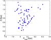 |
Fig. 23 Distribution in Galactic radius (Rnow) and height to the Galactic plane (Z) of the RAVE targets using the distances computed using PARAM. |
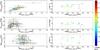 |
Fig. 24 Same as Fig. 22, but for RAVE DR5 seismic calibrated sample (see Kunder et al. 2017) and flagged as FLAG_G = 1. |
Means and dispersions of the difference between RAVE DR5 (general catalogue and seismic calibrated) and PARAM distances and reddening.
Finally, we also show the distances computed using only asteroseismology and magnitude, using the direct method described in Miglio et al. (2013): 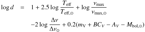 (6)where the solar values are the same adopted in Eq. (5), the Landolt V magnitude comes from APASS catalogue, AV is the Schlegel reddening, and the bolometric correction (BC) is taken from Girardi et al. (2002). The error on the distance determined using Eq. (6) was computed using propagation of uncertainty. The median uncertainty is of 10%, by taking into account the errors on Δν and νmax, temperature, magnitude and reddening. A comparison of the direct distances with distances provided by RAVE (DR4, DR5, and DR5 SC) and those computed in this work (PARAM) are shown in the bottom panel of Fig. 25. The distances computed using PARAM show good agreement with those computed with the direct method, while a larger dispersion is present in the RAVE DR4 distances, likely as a consequence of the different atmospheric parameters and their larger errors adopted and of the use of seismic information by PARAM. The typical error on distance of the previously mentioned methods is of 25% for DR4, 24% in DR5, 24% in DR5-SC and 4% in PARAM.
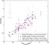 |
Fig. 25 Comparison of the distances obtained using asteroseismology and the direct method adopted in (Miglio et al. 2013), with the distances provided in RAVE (DR4, DR5 and DR5-SC) and the distances determined using PARAM (blue points). Typical errors of each method are shown in the top-left of the figure (both DR5 and DR5-SC have the same typical error). |
8. Conclusions
In this paper we analysed 87 RAVE stars with detected solar-like oscillations, observed during Campaign 1 of the K2 mission. The use of asteroseismic log (g) (with typical accuracy of 0.03 dex) and photometric temperature was able to break the log (g)-Teff degeneracy that affects the RAVE wavelength interval (around CaII Triplet, especially for red giants). By comparing our measurements with those of RAVE DR4, we were able to quantify the impact of the refined gravities and effective temperature obtained here on the elemental abundances, distances and reddening (and age) determinations for these stars.
Our results can be summarised as follows:
-
A difference between log (g)seismo and log (g)RAVEDR4 exists. This is a consequence of the resolution and short spectral coverage of the RAVE survey that leads to a strong log (g)-Teff degeneracy. This degeneracy had been partially solved in RAVE DR4 by adopting a decision-tree pipeline, together with a projection-method one. In this work we, provide a calibration for the gravity of RAVE DR4 red giants (Eq. (3)) that is valid for giants selected in the colour interval 0.50 ≤ (J−KS) ≤ 0.85.
The difference in log (g) leads, as expected, to differences with respect to the newly recomputed Teff, overall metallicity [M/H] and single element abundances. Stars with an overestimated gravity in DR4, have overestimated Teff and metallicity.
-
The change of the log (g) leads to a change of the star’s luminosity, affecting distances and reddening. A correct sample of red giants, with distances in agreement with the distances derived in this work, can be selected from RAVE DR4 by applying a colour cut 0.50 ≤ (J−KS) ≤ 0.85 and a very narrow cut in log (g), 2.5 ≤ log g ≤ 2.8 dex.
We determined a calibration for log (g) following Eq. (3), for photometrically selected giants in DR4. The same correction was used for the red giants in the forthcoming RAVE data release (DR5). In the RAVE DR5 catalogue, seismically calibrated gravities were provided for a sample of red giants, photometrically selected using 0.50 ≤ (J−KS)0 ≤ 0.85. These gravities appear in the “LOGG_SC” column. We also recommend recomputing abundances, metallicity and distances using the calibrated log (g). The shifts introduced by an uncertain log (g) assumption may introduce artefacts, such as metal-rich or metal-poor stars or stars with incorrect distance or kinematics. In the RAVE DR5 catalogue, this re-computation has already been performed.
The nature of these trends will be further explored in the other K2 Campaigns, increasing the statistics of our calibration sample and using RAVE stars possessing asteroseismology for Galactic archaeology investigations. Gaia will help to improve the atmospheric parameters as well. The strategy developed in this work can be used for the future parameter determination, by using the Teff and the log (g) coming from independent sources as priors (e.g. magnitude colours and parallaxes).
Acknowledgments
A.M., W.J.C., G.R.D., and Y.P.E. acknowledge the support of the UK Science and Technology Facilities Council (STFC). T.S.R. acknowledges support from CNPq-Brazil. This work has made use of the VALD database, operated at Uppsala University, the Institute of Astronomy RAS in Moscow, and the University of Vienna. Funding for RAVE has been provided by: the Australian Astronomical Observatory; the Leibniz-Institut fuer Astrophysik Potsdam (AIP); the Australian National University; the Australian Research Council; the French National Research Agency; the German Research Foundation (SPP 1177 and SFB 881); the European Research Council (ERC-StG 240271 Galactica); the Istituto Nazionale di Astrofisica at Padova; The Johns Hopkins University; the National Science Foundation of the USA (AST-0908326); the W. M. Keck foundation; the Macquarie University; The Netherlands Research School for Astronomy; the Natural Sciences and Engineering Research Council of Canada; the Slovenian Research Agency; the Swiss National Science Foundation; the Science & Technology Facilities Council of the UK; Opticon; Strasbourg Observatory; and the Universities of Groningen, Heidelberg and Sydney. The RAVE web site is at: https://www.rave-survey.org. We finally acknowledge the anonymous referee for the useful remarks.
References
- Anders, F., Chiappini, C., Minchev, I., et al. 2017a, A&A, in press DOI: 10.1051/0004-6361/201629363 [Google Scholar]
- Anders, F., Chiappini, C., Rodrigues, T. S., et al. 2017b, A&A, 597, A30 [NASA ADS] [CrossRef] [EDP Sciences] [Google Scholar]
- Baglin, A., Auvergne, M., Barge, P., et al. 2006, in The CoRoT Mission Pre-Launch Status, eds. M. Fridlund, A. Baglin, J. Lochard, & L. Conroy, ESA SP 1306, 33 [Google Scholar]
- Belkacem, K., Goupil, M. J., Dupret, M. A., et al. 2011, A&A, 530, A142 [NASA ADS] [CrossRef] [EDP Sciences] [Google Scholar]
- Bienaymé, O., Famaey, B., Siebert, A., et al. 2014, A&A, 571, A92 [NASA ADS] [CrossRef] [EDP Sciences] [Google Scholar]
- Bilir, S., Karaali, S., Ak, S., et al. 2012, MNRAS, 421, 3362 [NASA ADS] [CrossRef] [Google Scholar]
- Binney, J., Burnett, B., Kordopatis, G., et al. 2014, MNRAS, 437, 351 [NASA ADS] [CrossRef] [Google Scholar]
- Boeche, C., & Grebel, E. K. 2016, A&A, 587, A2 [NASA ADS] [CrossRef] [EDP Sciences] [Google Scholar]
- Boeche, C., Siebert, A., Williams, M., et al. 2011, AJ, 142, 193 [NASA ADS] [CrossRef] [Google Scholar]
- Boeche, C., Chiappini, C., Minchev, I., et al. 2013, A&A, 553, A19 [NASA ADS] [CrossRef] [EDP Sciences] [Google Scholar]
- Boeche, C., Siebert, A., Piffl, T., et al. 2014, A&A, 568, A71 [NASA ADS] [CrossRef] [EDP Sciences] [Google Scholar]
- Borucki, W. J., Koch, D., Basri, G., et al. 2010, Science, 327, 977 [NASA ADS] [CrossRef] [PubMed] [Google Scholar]
- Bressan, A., Marigo, P., Girardi, L., et al. 2012, MNRAS, 427, 127 [NASA ADS] [CrossRef] [Google Scholar]
- Brown, T. M., Gilliland, R. L., Noyes, R. W., & Ramsey, L. W. 1991, ApJ, 368, 599 [NASA ADS] [CrossRef] [Google Scholar]
- Bruntt, H., Basu, S., Smalley, B., et al. 2012, MNRAS, 423, 122 [NASA ADS] [CrossRef] [Google Scholar]
- Casagrande, L., Portinari, L., & Flynn, C. 2006, MNRAS, 373, 13 [NASA ADS] [CrossRef] [Google Scholar]
- Castelli, F., & Kurucz, R. L. 2004, IAU Symp., 210, Poster A20 [astro-ph/0405087] [Google Scholar]
- Cayrel, R., Depagne, E., Spite, M., et al. 2004, A&A, 416, 1117 [NASA ADS] [CrossRef] [EDP Sciences] [Google Scholar]
- Chiappini, C., Anders, F., Rodrigues, T. S., et al. 2015, A&A, 576, L12 [NASA ADS] [CrossRef] [EDP Sciences] [Google Scholar]
- Cutri, R. M., Skrutskie, M. F., van Dyk, S., et al. 2003, The IRSA 2MASS All Sky Catalog of point sources, 1/01 [Google Scholar]
- Cutri, R. M., Wright, E. L., Conrow, T., et al. 2013, Explanatory Supplement to the AllWISE Data Release Products, Tech. Rep. [Google Scholar]
- Da Costa, G. S., & Hatzidimitriou, D. 1998, AJ, 115, 1934 [NASA ADS] [CrossRef] [Google Scholar]
- da Silva, L., Girardi, L., Pasquini, L., et al. 2006, A&A, 458, 609 [NASA ADS] [CrossRef] [EDP Sciences] [Google Scholar]
- Davies, G. R., & Miglio, A. 2016, Astron. Nachr., 337, 774 [NASA ADS] [CrossRef] [Google Scholar]
- De Silva, G. M., Freeman, K. C., Bland-Hawthorn, J., et al. 2015, MNRAS, 449, 2604 [NASA ADS] [CrossRef] [MathSciNet] [Google Scholar]
- DENIS Consortium 2005, VizieR Online Data Catalog: II/263 [Google Scholar]
- Gilmore, G., Randich, S., Asplund, M., et al. 2012, The Messenger, 147, 25 [NASA ADS] [Google Scholar]
- Girardi, L., Bertelli, G., Bressan, A., et al. 2002, A&A, 391, 195 [NASA ADS] [CrossRef] [EDP Sciences] [Google Scholar]
- Handberg, R., & Lund, M. N. 2014, MNRAS, 445, 2698 [Google Scholar]
- Hawkins, K., Masseron, T., Jofre, P., et al. 2016, A&A, 594, A43 [NASA ADS] [CrossRef] [EDP Sciences] [Google Scholar]
- Heiter, U., Jofré, P., Gustafsson, B., et al. 2015, A&A, 582, A49 [NASA ADS] [CrossRef] [EDP Sciences] [PubMed] [Google Scholar]
- Hekker, S., Elsworth, Y., Mosser, B., et al. 2013, A&A, 556, A59 [NASA ADS] [CrossRef] [EDP Sciences] [Google Scholar]
- Holtzman, J. A., Shetrone, M., Johnson, J. A., et al. 2015, AJ, 150, 148 [NASA ADS] [CrossRef] [Google Scholar]
- Howell, S. B., Sobeck, C., Haas, M., et al. 2014, PASP, 126, 398 [NASA ADS] [CrossRef] [Google Scholar]
- Jorgensen, U. G., Carlsson, M., & Johnson, H. R. 1992, A&A, 254, 258 [NASA ADS] [Google Scholar]
- Kallinger, T., Weiss, W. W., Barban, C., et al. 2010, A&A, 509, A77 [NASA ADS] [CrossRef] [EDP Sciences] [Google Scholar]
- Kallinger, T., De Ridder, J., Hekker, S., et al. 2014, A&A, 570, A41 [NASA ADS] [CrossRef] [EDP Sciences] [Google Scholar]
- Kochukhov, O. P. 2007, in Physics of Magnetic Stars, eds. I. I. Romanyuk, D. O. Kudryavtsev, O. M. Neizvestnaya, & V. M. Shapoval, 109 [Google Scholar]
- Kochukhov, O. 2012, Astrophysics Source Code Library [record ascl: 1212.010] [Google Scholar]
- Kordopatis, G., Recio-Blanco, A., de Laverny, P., et al. 2011, A&A, 535, A106 [NASA ADS] [CrossRef] [EDP Sciences] [Google Scholar]
- Kordopatis, G., Gilmore, G., Steinmetz, M., et al. 2013, AJ, 146, 134 [NASA ADS] [CrossRef] [Google Scholar]
- Kunder, A., Kordopatis, G., Steinmetz, M., et al. 2017, AJ, 153, 75 [NASA ADS] [CrossRef] [Google Scholar]
- Kurucz, R. L. 2007, Robert L. Kurucz on-line database of observed and predicted atomic transitions [Google Scholar]
- Kurucz, R. L. 2014, Robert L. Kurucz on-line database of observed and predicted atomic transitions [Google Scholar]
- Lund, M. N., Handberg, R., Davies, G. R., Chaplin, W. J., & Jones, C. D. 2015, ApJ, 806, 30 [NASA ADS] [CrossRef] [Google Scholar]
- Majewski, S. R., Schiavon, R. P., Frinchaboy, P. M., et al. 2017, AJ, in press [arXiv:1509.05420] [Google Scholar]
- Martig, M., Rix, H.-W., Silva Aguirre, V., et al. 2015, MNRAS, 451, 2230 [NASA ADS] [CrossRef] [Google Scholar]
- Miglio, A., Chiappini, C., Morel, T., et al. 2013, MNRAS, 429, 423 [NASA ADS] [CrossRef] [Google Scholar]
- Miglio, A., Chaplin, W. J., Brogaard, K., et al. 2016, MNRAS, 461, 760 [NASA ADS] [CrossRef] [Google Scholar]
- Morel, T., & Miglio, A. 2012, MNRAS, 419, L34 [NASA ADS] [CrossRef] [Google Scholar]
- Morel, T., Miglio, A., Lagarde, N., et al. 2014, A&A, 564, A119 [NASA ADS] [CrossRef] [EDP Sciences] [Google Scholar]
- Mosser, B., & Appourchaux, T. 2009, A&A, 508, 877 [NASA ADS] [CrossRef] [EDP Sciences] [Google Scholar]
- Mosser, B., Barban, C., Montalbán, J., et al. 2011, A&A, 532, A86 [NASA ADS] [CrossRef] [EDP Sciences] [Google Scholar]
- Munari, U., Henden, A., Frigo, A., et al. 2014, AJ, 148, 81 [NASA ADS] [CrossRef] [Google Scholar]
- Pancino, E., Carrera, R., Rossetti, E., & Gallart, C. 2010, A&A, 511, A56 [NASA ADS] [CrossRef] [EDP Sciences] [Google Scholar]
- Pancino, E., et al. (Gaia-ESO Survey consortium) 2016, ASP Conf. Ser., 503, 275 [NASA ADS] [Google Scholar]
- Pasquini, L., Randich, S., Zoccali, M., et al. 2004, A&A, 424, 951 [NASA ADS] [CrossRef] [EDP Sciences] [Google Scholar]
- Pinsonneault, M. H., Elsworth, Y., Epstein, C., et al. 2014, ApJS, 215, 19 [NASA ADS] [CrossRef] [Google Scholar]
- Ralchenko, Y., Kramida, A., Reader, J., & NIST ASD Team 2010, NIST Atomic Spectra Database (ver. 4.0.0) [Online] [Google Scholar]
- Randich, S., Gilmore, G., & Gaia-ESO Consortium 2013, The Messenger, 154, 47 [NASA ADS] [Google Scholar]
- Rodrigues, T. S., Girardi, L., Miglio, A., et al. 2014, MNRAS, 445, 2758 [NASA ADS] [CrossRef] [Google Scholar]
- Ruchti, G. R., Fulbright, J. P., Wyse, R. F. G., et al. 2011, ApJ, 737, 9 [NASA ADS] [CrossRef] [Google Scholar]
- Siebert, A., Famaey, B., Minchev, I., et al. 2011, MNRAS, 412, 2026 [NASA ADS] [CrossRef] [Google Scholar]
- Soubiran, C., Le Campion, J.-F., Cayrel de Strobel, G., & Caillo, A. 2010, A&A, 515, A111 [NASA ADS] [CrossRef] [EDP Sciences] [Google Scholar]
- Steinmetz, M., Zwitter, T., Siebert, A., et al. 2006, AJ, 132, 1645 [NASA ADS] [CrossRef] [Google Scholar]
- Stello, D., Huber, D., Sharma, S., et al. 2015, ApJ, 809, L3 [NASA ADS] [CrossRef] [Google Scholar]
- Takeda, Y., & Tajitsu, A. 2015, MNRAS, 450, 397 [NASA ADS] [CrossRef] [Google Scholar]
- Takeda, Y., Tajitsu, A., Sato, B., et al. 2016, MNRAS, 457, 4454 [NASA ADS] [CrossRef] [Google Scholar]
- Thygesen, A. O., Frandsen, S., Bruntt, H., et al. 2012, A&A, 543, A160 [NASA ADS] [CrossRef] [EDP Sciences] [Google Scholar]
- Valdes, F., Gupta, R., Rose, J. A., Singh, H. P., & Bell, D. J. 2004, ApJS, 152, 251 [NASA ADS] [CrossRef] [Google Scholar]
- Valentini, M., Morel, T., Miglio, A., Fossati, L., & Munari, U. 2013, in European Physical Journal Web of Conferences, 43, 03006 [Google Scholar]
- Van Cleve, J. E., Howell, S. B., Smith, J. C., et al. 2016, PASP, 128, 075002 [NASA ADS] [CrossRef] [Google Scholar]
- van der Maaten, L., & Hinton, G. 2008, The Journal of Machine Learning Research, 9, 85 [Google Scholar]
- Wang, L., Wang, W., Wu, Y., et al. 2016, AJ, 152, 6 [NASA ADS] [CrossRef] [Google Scholar]
- Williams, M. E. K., Steinmetz, M., Binney, J., et al. 2013, MNRAS, 436, 101 [NASA ADS] [CrossRef] [Google Scholar]
- Yanny, B., Rockosi, C., Newberg, H. J., et al. 2009, AJ, 137, 4377 [NASA ADS] [CrossRef] [Google Scholar]
- Zhao, G., Zhao, Y.-H., Chu, Y.-Q., Jing, Y.-P., & Deng, L.-C. 2012, Res. Astron. Astrophys., 12, 723 [NASA ADS] [CrossRef] [Google Scholar]
- Zwitter, T., Siebert, A., Munari, U., et al. 2008, AJ, 136, 421 [NASA ADS] [CrossRef] [Google Scholar]
- Zwitter, T., Matijevič, G., Breddels, M. A., et al. 2010, A&A, 522, A54 [NASA ADS] [CrossRef] [EDP Sciences] [Google Scholar]
Appendix A: The χ2 fitting with a library of synthetic spectra
There are several causes to the rigid shift in metallicity pointed out in Sect. 4.2. It can be caused by incorrect continuum placement and by degeneracies, but also by incorrect assumption of the line parameters (e.g. loggf).
We identified some of these lines with incorrect loggf, as visible in Fig. A.1 and summarised in Table A.1.
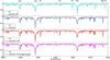 |
Fig. A.1 Comparison of the RAVE observed spectrum with a synthesised one for the benchmark star 551. From top to bottom: first panel, comparison of the real spectrum with the synthetic one, computed using the GAUFRE-NP parameters. Second panel: comparison of the real spectrum with the synthetic one computed using the literature parameters. Third panel: comparison of the real spectrum with the synthetic one built using the GAUFRE-TGP parameters. Bottom panel: comparison of the real spectrum with the synthetic one computed using the GAUFRE-GTP parameters and the loggf adopted in SP_Ace. |
Example of lines that possess incorrect loggf values in the VALD3 linelist and their loggf as in SP_Ace linelist.
Appendix B: The RAVE DR5 catalogue of seismic calibrated gravities for giant stars
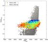 |
Fig. B.1 log (g)-Teffdiagram of the 105 102 seismic calibrated stars in RAVE_DR5, selected using FLAG_G = 1. The diagram is constructed using original DR5 parameters (grey dots) and DR5_SC parameters (coloured dots). DR5 data is coloured in grey-scale, with intensity following metallicity (metal-poor stars are light grey and dark grey marks metal-rich stars). The colour code for DR5_SC stars follows the standard scale, with metal-poor stars coloured in blue and metal-rich stars coloured in red. |
All Tables
Mean dispersions and offsets for Teff, log (g) and [ Fe / H ] of the GAUFRE pipeline with respect to the literature values for the calibration data set.
Mean dispersions and offsets for Teff, log (g) and [ Fe / H ] of the SPACE pipeline with respect to the literature values for the calibration data set.
Mean dispersions and offsets for Teff, log (g) and [ Fe / H ] of the GAUFRE pipeline with respect to the values measured by SP_Ace for the calibration data set.
Internal errors in atmospheric parameters and abundances in RAVE DR4 and those computed by combining spectroscopy and asteroseismology.
Selection criteria adopted in different works for creating the sample of red giants or red clump stars.
Means and dispersions of the difference between RAVE DR5 (general catalogue and seismic calibrated) and PARAM distances and reddening.
Example of lines that possess incorrect loggf values in the VALD3 linelist and their loggf as in SP_Ace linelist.
All Figures
|
Fig. 1 RA-Dec position of the targets observed by K2 during Campaign 1 (grey dots); the field is centred at 11:35:46 +01:25:02 and it was observed from 30-05-2014 to 21-08-2014. Empty red circles mark the RAVE stars observed by K2, while full red circles mark the 87 RAVE targets with detected oscillations. |
| In the text | |
|
Fig. 2 S/N distribution of the spectra of the 87 RAVE stars possessing asteroseismology. |
| In the text | |
|
Fig. 3 Distribution of Teff, log (g) and [M/H] of the RAVE stars analysed in this work. RAVE DR4 values are plotted in empty, red bars; the new atmospheric parameters derived using asteroseismology are plotted with blue, filled bars. |
| In the text | |
|
Fig. 4 Left panel: log (g)-Teff distribution of RAVE targets in K2-C1 target list (grey dots). Atmospheric parameters and errors are taken from RAVE DR4. Targets possessing Δν and νmax are colour-enhanced (by following calibrated [M/H] from RAVE DR4 catalogue) and circled in black. The dashed lines in log (g) mark the K2 detection limits at 2.1 and 3.35 dex. Right panel: Δν and νmax distribution of the 87 RAVE targets in K2-C1 possessing seismic parameters. The distribution is superimposed onto three Δν -νmax distributions calculated following Padova isochrones, taken at three different metallicities and ages. |
| In the text | |
|
Fig. 5 Comparison of the atmospheric parameters (from left to right: Teff, log (g) and [ Fe / H ] ) of the calibration set versus the values derived using the GAUFRE pipeline. Parameters were derived adopting four different strategies, following the same code as Fig. 7. Mean dispersions and offsets are displayed in Table 2. |
| In the text | |
|
Fig. 6 Comparison of the atmospheric parameters (from top to bottom: [ Fe / H ] , log (g) and Teff) measured by the GAUFRE pipeline, versus the atmospheric parameters available in the literature. Different symbols mark different approaches, following the same code as Fig. 7. Mean dispersions and offsets are displayed in Table 2. |
| In the text | |
|
Fig. 7 Comparison of the atmospheric parameters (from left to right: Teff, log (g) and [ Fe / H ] ) of the calibration set versus the values derived by using SP_Ace pipeline. Parameters were derived adopting four different strategies: with no prior (blue triangles), fixing the temperature to the real value (green squares), fixing the gravity (cyan stars) and fixing temperature and gravity (red circles). Mean dispersions and offsets are displayed in Table 3. |
| In the text | |
|
Fig. 8 Comparison of the atmospheric parameters (from top to bottom: [ Fe / H ] , log (g) and Teff) measured by the SP_Ace pipeline, versus the atmospheric parameters available in literature. Different symbols mark different strategies adopted for the analysis, following the same code as in Fig. 7. Mean dispersions and offsets are displayed in Table 3. |
| In the text | |
|
Fig. 9 Comparison of the atmospheric parameters (from left to right: Teff, log (g) and [ Fe / H ] ) of the calibration set atmospheric parameters as measured by GAUFRE versus the values derived with the SP_Ace pipeline. Parameters were derived adopting four different strategies: with no prior (blue triangles), fixing the temperature to the real value (green squares), fixing the gravity (cyan stars) and fixing temperature and gravity (red circles). Mean dispersions and offsets are displayed in Table 4. |
| In the text | |
|
Fig. 10 Comparison of the atmospheric parameters (from top to bottom: [ Fe / H ] , log (g) and Teff) measured by the SP_Ace pipeline, versus the atmospheric parameters measured by GAUFRE. Different symbols mark different strategies adopted for the analysis, following the same code as in Fig. 9. Mean dispersions and offsets are displayed in Table 4. |
| In the text | |
|
Fig. 11 Top panel: comparison between the Teff derived in this work, with and without asteroseismology (blue points and blue triangles respectively) and in RAVE DR4 (red points) versus the one obtained using APASS photometry (Munari et al. 2014). Bottom panel: comparison between the log (g) derived in this work, with and without asteroseismology (blue points and blue triangles, respectively) and in RAVE DR4 (red points) versus the one obtained using APASS photometry (Munari et al. 2014). |
| In the text | |
|
Fig. 12 Element variations when applying a variation to Teff and log (g) of ±150 K and ±0.50 dex. Differences between elements depend on the lines adopted and on the way their Curve of Growth (COG) depends on atmospheric parameters. |
| In the text | |
|
Fig. 13 Difference in log (g), Teff, [M/H] (calibrated and not calibrated) and [Mg/Fe] (Δ computed as RAVE DR4 − this work) for the 62 RAVE targets where the GAUFRE+Sp_Ace pipelines converged. In the top panel, the log (g) comparison, the fit used for calibrating log (g)RAVEDR4, is shown (red dashed line). |
| In the text | |
|
Fig. 14 t-SNE projection of approximately 420 000 RAVE spectra. The scaling in both directions is arbitrary, therefore the units on the axes are omitted. The colour-scale corresponds to the gravity of the stars as computed by Kordopatis et al. (2013). Giants are shown in red and dwarfs in blue. Lighter shaded hexagons include fewer stars than darker ones. Over-plotted black dots indicate locations of the stars from this study. |
| In the text | |
|
Fig. 15 Difference in log (g) (computed as log (g)RAVEDR4−log (g)seismo (empty circles) and log (g) |
| In the text | |
|
Fig. 16 Difference in log (g) (computed as log (g)RAVEDR4−log (g)APOGEE) vs. log (g)RAVEDR4 for the 855 RAVE targets in common with APOGEE-DR13. |
| In the text | |
|
Fig. 17 Difference in log (g) (computed as log (g)RAVEDR4 – log (g)GES) vs. log (g)RAVEDR4 for the 11 RAVE targets in common with GES. Triangles represent stars observed by GES using UVES, circles those observed using GIRAFFE instrument. |
| In the text | |
|
Fig. 18 Effective temperatures obtained in this work compared with those from the IRFM temperatures (blue dots), RAVE(DR4) (open circles) and RAVE(DR5) (red points). |
| In the text | |
|
Fig. 19 Differences in Teff, [M/H] (not calibrated and calibrated), [ Fe / H ] , [Mg/H], [Ni/H], [Ti/H] and [Si/H] vs. the differences in log (g). All differences are defined as RAVE(DR4) − (this work). The vertical dashed lines mark the | Δlog (g) | = 0.5 dex limits. |
| In the text | |
|
Fig. 20 Distributions of alpha-elements (Ni, Ti, Si, Al, Mg) plus Cr versus Fe of the RAVE stars analysed in this work. Filled blue dots are the abundances obtained by using asteroseismology, black circles are the original DR4 values. |
| In the text | |
|
Fig. 21 Metallicity distribution of RAVE DR5 seismic calibrated giants (RAVE-SC, see Kunder et al. 2017), compared with the MDF for the same stars but with DR5 metallicities. |
| In the text | |
|
Fig. 22 Comparison of distances, reddening (AV) and age derived using PARAM versus RAVE DR4 data. Data are colour-coded following the difference in gravity. Differences for the various quantities are always computed as: Δ = RAVE DR4 − this work. Top left panel: distances derived by PARAM vs. distance in RAVE DR4 (computed as the inverse of the parallax). Top right panel: distance residuals (in %) vs. log (g)seismo. Left central panel: AV derived by PARAM vs. AV present in RAVE DR4 catalogue. Right central panel: AV residuals vs. log (g)seismo. Bottom right panel: ages derived by PARAM vs. RAVE DR4 ones. Bottom left panel: age residuals (in %) vs. log (g)seismo. |
| In the text | |
|
Fig. 23 Distribution in Galactic radius (Rnow) and height to the Galactic plane (Z) of the RAVE targets using the distances computed using PARAM. |
| In the text | |
|
Fig. 24 Same as Fig. 22, but for RAVE DR5 seismic calibrated sample (see Kunder et al. 2017) and flagged as FLAG_G = 1. |
| In the text | |
|
Fig. 25 Comparison of the distances obtained using asteroseismology and the direct method adopted in (Miglio et al. 2013), with the distances provided in RAVE (DR4, DR5 and DR5-SC) and the distances determined using PARAM (blue points). Typical errors of each method are shown in the top-left of the figure (both DR5 and DR5-SC have the same typical error). |
| In the text | |
|
Fig. A.1 Comparison of the RAVE observed spectrum with a synthesised one for the benchmark star 551. From top to bottom: first panel, comparison of the real spectrum with the synthetic one, computed using the GAUFRE-NP parameters. Second panel: comparison of the real spectrum with the synthetic one computed using the literature parameters. Third panel: comparison of the real spectrum with the synthetic one built using the GAUFRE-TGP parameters. Bottom panel: comparison of the real spectrum with the synthetic one computed using the GAUFRE-GTP parameters and the loggf adopted in SP_Ace. |
| In the text | |
|
Fig. B.1 log (g)-Teffdiagram of the 105 102 seismic calibrated stars in RAVE_DR5, selected using FLAG_G = 1. The diagram is constructed using original DR5 parameters (grey dots) and DR5_SC parameters (coloured dots). DR5 data is coloured in grey-scale, with intensity following metallicity (metal-poor stars are light grey and dark grey marks metal-rich stars). The colour code for DR5_SC stars follows the standard scale, with metal-poor stars coloured in blue and metal-rich stars coloured in red. |
| In the text | |
Current usage metrics show cumulative count of Article Views (full-text article views including HTML views, PDF and ePub downloads, according to the available data) and Abstracts Views on Vision4Press platform.
Data correspond to usage on the plateform after 2015. The current usage metrics is available 48-96 hours after online publication and is updated daily on week days.
Initial download of the metrics may take a while.