| Issue |
A&A
Volume 600, April 2017
|
|
|---|---|---|
| Article Number | A140 | |
| Number of page(s) | 16 | |
| Section | Interstellar and circumstellar matter | |
| DOI | https://doi.org/10.1051/0004-6361/201629041 | |
| Published online | 14 April 2017 | |
Redistribution of CO at the location of the CO ice line in evolving gas and dust disks
1 Heidelberg University, Center for Astronomy, Institute of Theoretical Astrophysics, Albert-Ueberle-Straße 2, 69120 Heidelberg, Germany
e-mail: This email address is being protected from spambots. You need JavaScript enabled to view it.
2 Instituto de Astrofísica, Facultad de Física, Pontificia Universidad Católica de Chile, Santiago, Chile
3 Max Planck Institute for Astronomy, Königstuhl 17, 69117 Heidelberg, Germany
4 Harvard-Smithsonian Center for Astrophysics, 60 Garden Street, Cambridge, MA 02138, USA
5 School of Physics and Astronomy, The University of Leeds, E. C. Stoner Building, Leeds LS2 9JT, UK
6 Institute of Astronomy, University of Cambridge, Madingley Road, Cambridge, CB3 0HA, UK
7 University of Amsterdam, Astronomical Institute Anton Pannekoek, Postbus 94249, 1090 GE Amsterdam, The Netherlands
Received: 2 June 2016
Accepted: 5 January 2017
Abstract
Context. Ice lines are suggested to play a significant role in grain growth and planetesimal formation in protoplanetary disks. Evaporation fronts directly influence the gas and ice abundances of volatile species in the disk and therefore the coagulation physics and efficiency and the chemical composition of the resulting planetesimals.
Aims. In this work, we investigate the influence of the existence of the CO ice line on particle growth and on the distribution of CO in the disk.
Methods. We include the possibility of tracking the CO content and/or other volatiles in particles and in the gas in our existing dust coagulation and disk evolution model and present a method for studying evaporation and condensation of CO using the Hertz-Knudsen equation. Our model does not yet include fragmentation, which will be part of further investigations.
Results. We find no enhanced grain growth immediately outside the ice line where the particle size is limited by radial drift. Instead, we find a depletion of solid material inside the ice line, which is solely due to evaporation of the CO. Such a depression inside the ice line may be observable and may help to quantify the processes described in this work. Furthermore, we find that the viscosity and diffusivity of the gas heavily influence the re-distribution of vaporized CO at the ice line and can lead to an increase in the CO abundance by up to a factor of a few in the region just inside the ice line. Depending on the strength of the gaseous transport mechanisms, the position of the ice line in our model can change by up to ~ 10 AU and consequently, the temperature at that location can range from 21 to 23 K.
Key words: protoplanetary disks / accretion, accretion disks / diffusion / methods: numerical
Member of the International Max Planck Research School for Astronomy and Cosmic Physics at the Heidelberg University. PUC-HD Graduate Student Exchange Fellow.
Royal Society Dorothy Hodgkin Fellow.
© ESO, 2017
1. Introduction
Ice lines are locations in protoplanetary disks at which a transition between the gaseous and the solid phase of an element or a molecular species occurs. Inwards of the ice line, the volatile species is condensed in the form of ice. Outside the ice line, the material exists in its solid form. Ice lines are of special interest in planetary sciences since they are suggested to affect the formation and composition of planetesimals (Öberg et al. 2011). Ali-Dib et al. (2014) argue from the chemical composition of Uranus and Neptune that they may have been formed at the carbon monoxide ice line.
Planetesimals are formed from dust and ice surrounding young stars in protoplanetary disks. The dust particles collide and are held together by contact forces forming ever larger bodies (see, e.g., Brauer et al. 2008; Birnstiel et al. 2010). However, experiments and simulations show that the growth is limited by at least two processes. One is the inward drift of particles on Keplerian orbits losing angular momentum to the pressure-supported gas orbiting the star with sub-Keplerian velocities (Weidenschilling 1977). The drift velocity is size-dependent. Therefore, particles affected by drift quickly fall onto the central star. Another mechanism that prevents grain growth is fragmentation. If the collision velocity is high enough, silicate particles tend to bounce or fragment rather than sticking together (Blum & Wurm 2008). If particles grow to certain sizes (centimeter to decimeter), the streaming instability can take over and form planetesimals by clumping and subsequent gravitational collapse (see, e.g., Johansen et al. 2007; Youdin & Goodman 2005; Bai & Stone 2010; Drążkowska & Dullemond 2014).
How particles can grow to sizes for which the streaming instability is efficient is unknown. Besides the fact that icy materials have higher fragmentation velocities than pure silicate particles (Wada et al. 2009; Gundlach & Blum 2015), and can therefore grow to larger sizes, several authors argue that ice lines play an important role in the growth process (e.g., Kretke et al. 2008; Brauer et al. 2008). Also, Kataoka et al. (2013) proposed that fluffy ice aggregates may overcome the drift barrier. Stevenson & Lunine (1988) found, in their model, a significant solid material enhancement at the ice line due to diffusive redistribution of vapor from the inner disk and subsequent condensation on particles outside the ice line. Closely related, Ros & Johansen (2013) proposed grain growth by evaporation of inward-drifting particles and subsequent recondensation of backwards-diffusing vapor. Cuzzi & Zahnle (2004) proposed a significant vapor enhancement inside the ice line due to rapidly inward-drifting particles.
The goal of our work is to include the transport of volatile materials into the grain growth and disk model of Birnstiel et al. (2010) and to use this model to investigate the influence of possible particle density enhancements at ice lines on dust coagulation and on the distribution of CO gas. We therefore developed a model to track the volatile content of particles and the gas including the processes of coagulation, radial drift, and viscous accretion, as well as CO evaporation and condensation at the ice line.
We focus, here, on CO ice near the CO ice line for several reasons. First, we assume that the collisional physics of the particles is mostly determined by the presence of water ice. If we further assume that the water ice content is always well mixed within the particle, there will always be enough water ice at the particle’s surface such that the collisional physics does not change by crossing the CO ice line and evaporating the CO (but see also Okuzumi et al. 2016). Wada et al. (2009) estimated the fragmentation velocity of water ice particles to be ~ 50 m/s. Such high collision velocities are not reached in our model. We can therefore neglect fragmentation, since, even by total evaporation of the CO, there is still enough water ice in the particles such that we can use the higher fragmentation velocity of water ice. The growth of the particles is therefore solely limited by the inward drift. But see also Gundlach & Blum (2015), who found fragmentation velocities for water ice in the order of 10 m/s. It might also be the case that the water ice is not well mixed within the particle or that the particle is covered by a layer of CO. In that case, the fragmentation velocity is that of CO ice, which might also be lower than the fragmentation velocity of water ice. We aim to investigate the influence of fragmentation in future works.
Another reason for looking at CO is that it has observable features (Qi et al. 2015). The CO ice line at temperatures of approximately 20 K is in the outer parts of protoplanetary disks compared to other volatile species such as water ice. Furthermore, the CO abundance is generally large enough to be well observed.
We investigate the radial distribution of dust particles and molecular species in the gas and ice phases around the region of the ice line in a time dependent manner by solving the Smoluchowski equation and the re-distribution of the CO vapor originating from the evaporating particles.
In Sect. 2, we describe our model of advection, diffusion, grain growth, and evaporation/condensation. In Sect. 3, we show the influence of the ice line on the grain growth and the influence of the advection and diffusion of the gas on the CO vapor distribution at the ice line. In Sect. 4, we discuss our results and the assumptions made in the model.
2. Model
We constructed a model for simulating the evolution of a viscously evolving protoplanetary disk including dust coagulation, particle drift, condensation, and evaporation of CO at the CO ice line. The model is one-dimensional and the densities are vertically integrated, assuming that gas and dust are constantly in thermal equilibrium, throughout the model. We model the surface densities of approximately 150 different dust sizes Σdust,i and of two gas species, ΣH2 and ΣCO. Our model of CO transport is built upon the gas and dust model of Birnstiel et al. (2010).
The gas disk is viscously evolving according the α-disk model of Shakura & Sunyaev (1973) while we study the diffusive behavior of CO by choosing different values for the Schmidt number Sc, which is the ratio of viscosity over diffusivity of the gas.
We model dust growth by solving the Smoluchowski equation. The dust species themselves are subject to radial drift and gas drag. In contrast to previous works, we use a two-dimensional scalar field for the particle distribution, where one dimension is the silicate mass and the second dimension the CO ice content of the particle. We therefore model the migration of CO both via drifting particles and via diffusing gas and simulate the evaporation of CO at the CO ice line by solving the Hertz-Knudsen equation.
2.1. Evolution of the gas surface density
We consider two molecular gas species in our model, H2, which is the main gas density constituent, and CO, which is generally the second most abundant molecular species in the interstellar medium (ISM). The surface density of the two species, ΣH2 and ΣCO, and therefore the total gas density, Σgas, are directly related through the continuity equation:  (1)where ugas is the radial gas velocity given by Lynden-Bell & Pringle (1974):
  (2)where ν is the viscosity of the gas. Shakura & Sunyaev (1973) parameterized the viscosity in their α-disk model to account for an unknown source of viscosity with
  (3)where cs is the sound speed, HP = cs/ ΩK the pressure scale height of the disk, and ΩK the Keplerian frequency. The viscosity parameter α is typically of the order of 10-2 to 10-4 (e.g., Johansen & Klahr 2005). Equation (1) has no source terms on the right hand side, because we do not consider any infall of matter from the common envelope onto the disk. Evaporation and condensation, which would also be a source or sink term for ΣCO, are treated separately.
We assume that both gas species evolve separately without interacting with one another. We then obtain a separate continuity equation for each of the species j![Mathematical equation: \begin{equation} \frac{\partial}{\partial t} \Sigma_j = -\frac{3}{R}\frac{\partial}{\partial R} \left[ \sqrt{R} \frac{\partial}{\partial R} \left( \Sigma_j \nu \sqrt{R} \right) \right]. \label{eqnViscAccr} \end{equation}](/articles/aa/full_html/2017/04/aa29041-16/aa29041-16-eq22.png) (4)Following the calculations of Pavlyuchenkov & Dullemond (2007), this equation can be further manipulated to
(4)Following the calculations of Pavlyuchenkov & Dullemond (2007), this equation can be further manipulated to ![Mathematical equation: \begin{eqnarray} \begin{split} \frac{\partial}{\partial t} \Sigma_j &= -\frac{3}{R}\frac{\partial}{\partial R} \left[ \sqrt{R} \frac{\partial}{\partial R} \left( \Sigma_\mathrm{gas} \frac{\Sigma_j}{\Sigma_\mathrm{gas}} \nu \sqrt{R} \right) \right] \\ &= -\frac{3}{R}\frac{\partial}{\partial R} \left[ \sqrt{R} \frac{\Sigma_j}{\Sigma_\mathrm{gas}} \frac{\partial}{\partial R} \left( \Sigma_j \nu \sqrt{R} \right) + R \Sigma_\mathrm{gas} \nu \frac{\partial}{\partial R} \left( \frac{\Sigma_j}{\Sigma_\mathrm{gas}} \right) \right], \end{split} \end{eqnarray}](/articles/aa/full_html/2017/04/aa29041-16/aa29041-16-eq23.png) (5)where Σgas = ∑ jΣj is the total gas surface density. By substituting the gas velocity of Eq. (2) in this equation, we obtain
(5)where Σgas = ∑ jΣj is the total gas surface density. By substituting the gas velocity of Eq. (2) in this equation, we obtain ![Mathematical equation: \begin{equation} \frac{\partial}{\partial t} \Sigma_j + \frac{1}{R} \frac{\partial}{\partial R} \left( R \Sigma_j u_\mathrm{gas} \right) -\frac{3}{R} \frac{\partial}{\partial R} \left[ R \Sigma_\mathrm{gas} \nu \frac{\partial}{\partial R} \left( \frac{\Sigma_j}{\Sigma_\mathrm{gas}} \right) \right] = 0. \label{eqnGasAdvStandard} \end{equation}](/articles/aa/full_html/2017/04/aa29041-16/aa29041-16-eq25.png) (6)This equation implies that each gas species is radially advected with the gas velocity ugas and has a diffusive term, which smears out concentrations.
(6)This equation implies that each gas species is radially advected with the gas velocity ugas and has a diffusive term, which smears out concentrations.
By introducing the Schmidt number Sc = ν/D, which is the ratio of viscosity ν to diffusivity D of a gas, one can disentangle advection and diffusion ![Mathematical equation: \begin{equation} \frac{\partial}{\partial t} \Sigma_j + \frac{1}{R} \frac{\partial}{\partial R} \left( R \Sigma_j u_\mathrm{gas} \right) -\frac{1}{R} \frac{\partial}{\partial R} \left[ R \Sigma_\mathrm{gas} D \frac{\partial}{\partial R} \left( \frac{\Sigma_j}{\Sigma_\mathrm{gas}} \right) \right] = 0. \label{eqnGasAdv} \end{equation}](/articles/aa/full_html/2017/04/aa29041-16/aa29041-16-eq28.png) (7)A Schmidt number of Sc = 1/3 reproduces Eq. (6). Physically, the Schmidt number is the ratio of momentum transport to pure-mass transport. By changing Sc and keeping α constant, we investigate the influence of the diffusivity D on the CO distribution in the disk.
(7)A Schmidt number of Sc = 1/3 reproduces Eq. (6). Physically, the Schmidt number is the ratio of momentum transport to pure-mass transport. By changing Sc and keeping α constant, we investigate the influence of the diffusivity D on the CO distribution in the disk.
2.1.1. Vertical and radial structure of the gas disk
We assume that the gas is always in thermal equilibrium and that the temperature profile does not change over time. The vertical structure of the gas density is then given by ![Mathematical equation: \begin{equation} \rho_\mathrm{gas} \left( z \right) = \rho_\mathrm{gas} \left( z=0 \right) \ \exp \left[ - \frac{1}{2} \frac{z^2}{H_\mathrm{P}^2} \right], \label{eqnGasVertStruct} \end{equation}](/articles/aa/full_html/2017/04/aa29041-16/aa29041-16-eq30.png) (8)where z is the height above the midplane. Since Σgas is the z-integral of ρgas, it follows directly for the midplane gas density that
(8)where z is the height above the midplane. Since Σgas is the z-integral of ρgas, it follows directly for the midplane gas density that  (9)Even though the model is one-dimensional, we still need the vertical structure of the disk to calculate the densities at the midplane that are needed for the coagulation as well as for the evaporation method.
In our fiducial model, we used the following power law as initial surface density distribution:  (10)
(10)
2.1.2. Temperature structure of the disk
For the midplane temperature of the disk, we assume a simple power law;  (11)that remains constant in time. The viscous heating rate, which is the energy that is created by the viscous accreting of the gas, is proportional to the gas density Σgas (Nakamoto & Nakagawa 1994) and therefore mainly important in the inner part of the disk. Since we are interested in the region of the CO ice line at 40–50 AU where the densities are low, this effect is negligible.
2.2. Radial evolution of the dust surface density
The spatial evolution of the dust particles is strongly influenced by interactions with the gas. Although it is possible, in real disks, that particles become locally concentrated to gas-to-dust ratios of unity or less, especially at the disk’s midplane, and therefore trigger streaming instabilities, we neglect this here, and assume that accumulations of dust happen only at smaller radii (Youdin & Shu 2002) or on smaller scales (Youdin & Goodman 2005). In other words: the gas has an effect on the dust particles, but the dust particles have no back-reaction on the gas in our model.
To describe the coupling of the particles to the gas, it is useful to characterize the particles not by size but by their dimensionless Stokes number St. The Stokes number is defined as the ratio of the stopping time τs of the particles to the largest eddy’s turn-over time τed;  (12)The Stokes number can be used as a measure to describe the coupling between the gas and the dust. Since this coupling depends not solely on the particle size but, amongst other parameters, also on the gas density, it is convenient to use the Stokes number to describe the equations of motion of the particles.
The stopping time τs in Eq. (12) is the ratio between a particle’s momentum and the rate of its momentum change by the drag force. It yields the time scale on which a particle adapts to the gas velocity. Weidenschilling (1977) identified four different regimes of the drag force. The important regime in our work is the Epstein regime, where the stopping time is given by  (13)with the bulk density of the solids ρs and the particle size a.
  is the mean thermal velocity of the gas molecules. In protoplanetary disks, the Stokes I drag regime is important only in the inner part of the disk (≲1 AU). We therefore only include the Epstein regime in this work.
As a first order approximation for the eddy turnover time, one can use τed = 1/ΩK (Schräpler & Henning 2004), and obtain the Stokes number:  (14)The advection of the dust surface densities of the different species can now be described with a continuity equation as Eq. (7)
 ![Mathematical equation: \begin{equation} \frac{\partial}{\partial t} \Sigma_{\mathrm{dust},i} + \frac{1}{R} \frac{\partial}{\partial R} \left( R \left[ \Sigma_{\mathrm{dust},i} u_{\mathrm{dust},i} - D_{\mathrm{dust},i} \Sigma_\mathrm{gas} \frac{\partial}{\partial R} \frac{\Sigma_{\mathrm{dust},i}}{\Sigma_\mathrm{gas}} \right] \right) = 0, \label{eqnDustCont} \end{equation}](/articles/aa/full_html/2017/04/aa29041-16/aa29041-16-eq47.png) (15)where Ddust,i = αcsHP/ (1 + St2) is the dust diffusivity and udust,i the radial velocity of dust species i given by
(15)where Ddust,i = αcsHP/ (1 + St2) is the dust diffusivity and udust,i the radial velocity of dust species i given by  (16)This velocity consists of two terms. The first term describes the dust particles that are dragged along with the inwards accreting gas; it is most effective for small particles
  that are well-coupled to the gas and insignificant for large particles
  . The second term describes radial drift due to a pressure gradient in the gas. The gas feels an additional force due to its own pressure gradient. If the pressure gradient is pointing inwards, then the gas is on a sub-Keplerian orbit. The acceleration of the dust particles due to the pressure force, on the other hand, is negligible because of their high bulk density compared to the gas. Therefore, the particles try to orbit with a Keplerian velocity. Due to this velocity difference with the gas, they feel a constant headwind, lose angular momentum, and drift in the direction of the pressure gradient. The maximal drift velocity (for particles with St = 1) is given by Weidenschilling (1977) as
  (17)
(17)
2.3. Vertical structure of the dust disk
Since the dust particles do not feel any pressure amongst themselves, we cannot give a simple pressure-equilibrium expression for the particle scale heights as for the gas scale height HP. The particle scale heights are given by the equilibrium of vertical settling by gravity and turbulent stirring and therefore depend on the particle’s Stokes number. Therefore, every particle size has its own scale height. We follow, here, Brauer et al. (2008) for the description of the scale height of species i as  (18)which limits the dust scale height to be, at maximum, equal to the gas scale height HP. From this equation, it can be seen that larger particles are settled to the midplane, while small particles follow the gas scale height. A stronger turbulence (i.e., larger turbulent viscosity parameter α), in general, increases the scale height up to a maximum of HP.
We assume that the particles are distributed with Gaussian distributions just as the gas in Eq. (8), but with the dust particle’s specific scale height hi instead, which allows us to analytically integrate the Smoluchowski equation vertically.
2.4. Dust coagulation
We include dust growth in our model to study the CO redistribution in protoplanetary disks. The dust carries the CO ice inwards through the CO ice line. As seen in Eq. (16), the Stokes number, and therefore the particle size, is important for the drift velocity of the dust particles.
We therefore include hit-and-stick collisions of particles in our model. We neglect fragmentation because the CO ice line is well outside of the water ice line, meaning that, everywhere in our model, the particles have a significant amount of water ice, which is also mixed within the particle in such a way that the particle collision properties are always determined by the water ice. As explained above, we therefore neglect fragmentation.
2.4.1. Smoluchowski equation
The growth of the dust particles with mass m by hit-and-stick collisions without fragmentation can be described by the Smoluchowski equation  (19)where the collision kernel K(m;m′) = σgeo(m;m′)Δu(m;m′) is the product of the geometrical cross section and the relative velocity of the colliding particles. Equation (19) is a partial differential equation for the time evolution of a mass distribution of particles. The positive term on the right-hand side counts collisions that lead to particles of mass m. The negative term removes particles of mass m that collided with other particles to create larger particles.
To keep track of not only the mass of the particles, but also of another property that represents the CO ice content of them, we add another parameter Q to our distribution. The following equations are general for an arbitrary Q that could represent anything from the volume of the particle as in Okuzumi et al. (2009) to the electrical charge of the particle. In the following sections we identify Q with the particle’s ice fraction. The two-dimensional Smoluchowski equation then reads as follows  (20)where Qnew(m′,Q′;m′′,Q′′) is the new Q-value of the particle that was created in the collision. In principle, this equation could be solved as for Eq. (19), but adding another parameter and therefore two additional integrals would be computationally very expensive.
We therefore follow the moment method introduced by Okuzumi et al. (2009) to re-write one two-dimensional Smoluchowski equation into two one-dimensional equations. The idea is that instead of evolving the full Q- distribution, we only evolve its first moment, its mean  for a given mass m. By introducing the distribution function of particles of mass m
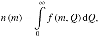 (21)and the mean Q-value of particles with mass m
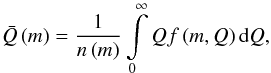 (22)and by assuming that the particle distribution is very sharp in Q
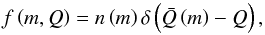 (23)where δ is the Dirac delta function, Eq. (20) can be rewritten and simplified. We end up with one partial differential equation for
 (24)and one equation for
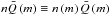
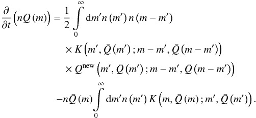 (25)For a detailed derivation of the equations, we refer to Okuzumi et al. (2009). Both one-dimensional equations can be simultaneously solved, which is significantly more efficient than solving one two-dimensional equation. The coagulation Eqs. (24) and (25) and the dust advection Eq. (7) are simultaneously solved with the method described in the appendix of Birnstiel et al. (2010)
2.4.2. The Q-parameter
We have now the freedom of choice on what exactly the physical meaning of our Q-parameter should be. One way to include ices in our coagulation code is to take m = mtot as the total mass and  as the ice fraction of a particle. However, this approach has the disadvantage that as a result of evaporation and condensation, both parameters m and Q change. In this case, evaporation/condensation would be advection of the function Q(m,t) in the m-coordinate with an additional source term.
We therefore chose m = msil as the silicate mass and  as the ice fraction of a particle. Here, evaporation and condensation only change Q and not m.
By using this approach, the ice mass of a particle is  , whereas the total mass is
  . Therefore, we cannot model particles fully consisting of ice (Q = 1). Qnew, which is the new Q-value of a particle resulting from a collision followed by sticking between a particle with mass m and another particle with mass m′ (and ice fractions Q and Q′, respectively), is then determined by
 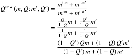 (26)
(26)
2.4.3. Relative velocities
The coagulation is driven by the relative velocities of the particles that determine the collision rates and the possible collision outcome. We consider, here, five different sources of relative velocities: Brownian motion ΔuBM, azimuthal particle drift Δuφ, radial particle drift ΔuR, vertical settling Δusett, and turbulence Δuturb.
The total relative velocity is then given by the root mean square of all sources of relative velocity 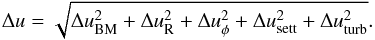 (27)We assume that all particles of a certain size collide with this distinct mean velocity. It has been shown that the use of a velocity distribution can have a significant influence on dust growth by breaking through growth barriers as the bouncing barrier or the fragmentation barrier (Windmark et al. 2012; Garaud et al. 2013). Since we are not dealing with bouncing and/or fragmentation in this model, we do not consider any velocity distribution.
For a detailed description of the various sources of relative velocity, we refer to Birnstiel et al. (2010).
2.5. Evaporation and condensation
When particles drift inwards they move from colder regions in the disk to warmer regions. At some point – at the ice line – the temperature is high enough for the ice in the particles to be evaporated. The vapor that is created by evaporation can then be diffused backwards through the ice line and can re-condense on the colder particles there. We therefore consider both evaporation and condensation along with diffusion and viscous evolution of the gas in our model.
We assume that the particles always adapt instantaneously to the new temperature. This might not be the case for very large particles with high heat capacities. But as seen later in Sect. 3, we do not have such large particles. The temperature change our particles experience is solely caused by their drift from colder regions to warmer regions in the disk. With typical drift speeds, the particles experience a change in temperature of less than 1 K in 1000 yr. The assumption of instantaneous adaption to the ambient temperature is therefore well justified.
Evaporation/condensation can be described by the Hertz-Knudsen equation which gives the number of CO molecules N per unit surface area that leave the particle, 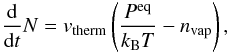 (28)where nvap is the number density of vapor molecules, Peq the saturation pressure of the volatile species and
 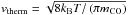 is the mean thermal velocity of gas molecules of mass mCO. If the ambient pressure of the volatile species equals the saturation pressure then there is no net evaporation.
Peq has to be determined experimentally. We use the values from Leger et al. (1985) as ![Mathematical equation: \begin{equation} P^\mathrm{eq}_\mathrm{CO} \left( T \right) = 1 \frac{\mathrm{dyn}}{\mathrm{cm}^2} \times \exp \left[ -\frac{1030\ \mathrm{K}}{T} + 27.37 \right]. \end{equation}](/articles/aa/full_html/2017/04/aa29041-16/aa29041-16-eq98.png) (29)Evaporation/condensation is, in general, dependent on the surface curvature of the particle, where convex surfaces have slightly higher evaporation rates than concave surfaces (Sirono 2011). We do not consider those surface curvature effects in our model. This means if Eq. (28) is negative, we have condensation on all particles independent of their size. If Eq. (28) is positive, all particles evaporate as long as they still carry some ice.
(29)Evaporation/condensation is, in general, dependent on the surface curvature of the particle, where convex surfaces have slightly higher evaporation rates than concave surfaces (Sirono 2011). We do not consider those surface curvature effects in our model. This means if Eq. (28) is negative, we have condensation on all particles independent of their size. If Eq. (28) is positive, all particles evaporate as long as they still carry some ice.
The Hertz-Knudsen equation needs to be solved for every particle size at every radial and vertical position of the disk separately and simultaneously. But since we are not dealing with the vertical structure of the disk in our model, we need to transfer this expression into an expression for surface densities. If we look at the midplane of the disk, the Hertz-Knudsen equation for the midplane vapor mass density reads as 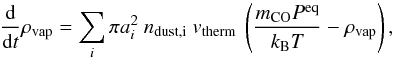 (30)where ai is the particle radius and ndust,i the midplane number density of dust particles species i. This system is in equilibrium if
 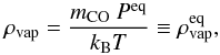 (31)where
  is defined as the equilibrium vapor mass density. If we assume that the vapor is always in pressure equilibrium, we get for the equilibrium vapor surface density
  (32)Assuming this, we can transform Eq. (30) into an expression for the vapor surface density
  (33)with
  Therefore, the change in the ice surface density of particle species i is given by
  (36)which is the difference between a condensation term CiΣvap and an evaporation term Ei. The deeper meaning behind this formalism is that we treat the evaporation/condensation rates as if the particles were in the midplane, while we assume that gas and particles are always in thermal equilibrium and distributed according to their pressure scale heights HP and hi.
For Ci and Ei, the following relation holds:  (37)
(37)
2.5.1. Condensation mode
If S > 0, then we are in the condensation regime and condensation will take place on all particles. In that case, we can directly integrate Eqs. (36) and (33) until the end of the time step. If we assume that the particle radius ai is constant and does not change over the time step, then both equations have analytic solutions. This assumption is justified if we use a canonical abundance of CO of 10-4. By using a dust to gas ratio of 10-2, this leads to an initial mass ratio of CO (gas and ice phase) to dust of ~ 14%, and therefore a maximal change in radius of ~5%. The analytic solution of Eq. (33) is then  (38)Using Eq. (38) in Eq. (36) leads to
  (39)where in the last step, Eq. (37) was used. This equation has the analytical solution
  (40)Equations (38) and (40) can be used to calculate the surface densities at any time step directly.
2.5.2. Evaporation mode
If at the start of the time step S < 0, we are in an evaporation regime. Also in this regime, the time evolution is governed by Eqs. (38) and (40). However, we need to take into account that bare grains will not contribute to the flux of molecules, and that during the time step, grains may become bare. Therefore, we split the integration into a number of sub-steps. During each sub-step, the same set of grain sizes contributes to the evaporation flux, and we completely ignore bare grains. For each step, we define restricted versions of C and E. These restricted versions only sum over non-bare grains;  (41)We define bare grains as particles that have less than one mono-layer of ice molecules on their surface.
With these definitions, we use Eq. (40) to check if any ice component becomes depleted during the time step, that is, we check for the first root in any of the equations; 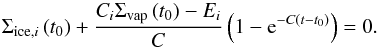 (42)If that first root is before the end of the time step, we evolve the system to this time, remove the newly bare grain size from the participating set of grain sizes, and continue in the same way. Eventually, either all grains will be bare, or the first root in the set of Eqs. (42) will be beyond the end of the time step. Then we use Eq. (40) with C replaced by Crest to move the system to the end of the time step.
2.5.3. Caveats
We do not consider grain curvature effects on evaporation and condensation. This means either all particles are in evaporation mode or all particles are in condensation mode. In general, this effect is mostly effective for very small particles (<0.1 μm). As seen in Sect. 3, we get rid of the small particles very quickly due to coagulation and do not replenish them since we do not have fragmentation.
The surface of a real disk is directly illuminated by the star and therefore hotter than the midplane. This means that in addition to a radial ice line in the midplane, disks also have a two-dimensional surface called atmospheric ice line towards their surface, where the temperatures are high enough for ices to evaporate. Since we are only looking at midplane quantities to decide between evaporation or condensation, we neglect the atmospheric ice line. This leads to an overestimation of the ice content of the particles. But since most of the dust mass is basically below the vertical ice line, especially the larger grains, the effect is only expected to be important near the radial ice line where the vertical ice line reaches the midplane. However, this is a radially narrow region, so it shouldn’t affect the global transport, but possibly modifies the shape of the snow line.
Our particles have a relatively simple structure in the model. They are treated as particles with a core and a mantle of CO. If two particles with mantles collide in our model, they form a new particle with a single core and a mantle instead of a particle with two cores connected at their contact point, or even more complex fragmented structures. This may lead to an artificial growth of silicate particles. If we consider the case where outside the ice line, many particles with CO mantles collide; in our model they form a large particle with a large single core and a large CO mantle. By crossing the ice line and evaporating the CO, we are then left with this large core instead of many small cores. Aumatell & Wurm (2011) showed, experimentally, that by evaporating fractal ice particles, one would expect to be left with many small particles instead of one large particle. In favor of simplicity, we neglect this effect.
Furthermore, the evaporation of CO ice can be decreased if some of the CO ice is trapped inside a porous and spatially complex structure of the dust particle. Or it can be increased if the dust particle is very fluffy because its surface area is then much larger than in the case of a spherical particle of the same size. These effects are also ignored in this work.
3. Results
3.1. The fiducial model
Fiducial model parameters.
The input quantities of our fiducial model are given in Table 1. The grain sizes are initially distributed with the MRN distribution (Mathis et al. 1977) with an upper cutoff at 1 μm. We integrate the Eqs. (7), (15), (24), and (25) and use the method for evaporation/condensation as described in Sect. (2.5) to calculate the time evolution of the gas surface densities ΣH2and ΣCO, and the dust surface densities of the different grain sizes Σdust,j.
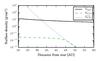 |
Fig. 1 Gas surface densities of the fiducial model after 1 Myr. Shown are the total gas surface density (solid black line) and the surface density of gaseous CO (dashed green line). The dotted blue line is the equilibrium surface density of CO given by Eq. (32). The location where the CO surface density detaches from the equilibrium CO surface density is called the ice line. |
Figure 1 shows the gas surface densities after 1 Myr of the simulation. We have chosen this value, because it is the typical age of some of the best studied star-forming regions and thus also of the disks therein. Also, it is the typical timescale for disk dispersion (e.g., Haisch et al. 2001). Shown is the total gas surface density Σgas = ΣH2 + ΣCO and the CO gas surface density ΣCO. Overplotted is the equilibrium CO gas surface density  given by Eq. (32), which the system would have if there was no net evaporation/condensation and if there was enough CO available. If there is not enough CO in the system, then the CO in the particles evaporates until the grains are bare. The radial distance, where ΣCO detaches from , is then our definition of the CO ice line because it is the point where there is just enough CO in our model to provide the vapor pressure necessary to counterbalance the evaporation. In our fiducial model, this happens at ~ 47 AU. Outside the ice line, the CO is frozen out onto the grains until
  . Inside the ice line, all CO is in the gas phase. Although it is not a power law, the equilibrium density at the position of the ice line can be approximated by
  with p ≈ 20. Since this is very steep, the region around the ice line, where the CO is partially condensed, is very small and therefore the ice line is well defined.
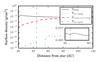 |
Fig. 2 Dust surface densities of different dust sizes at the CO ice line after 1 Myr. Shown are the total surface density (solid gray line), millimeter-sized (dotted blue line), sub-millimeter-sized (dashed red line), and sub-micrometer-sized (dash-dotted green line) particles. The vertical dashed line marks the location of the CO ice line. |
Figure 2 shows the total dust surface density Σdust and the surface densities Σa > 1 mm of grains larger than one millimeter, Σ1 μm <a < mm of grain sizes between 1 mm and 1 μm, and Σa < 1 μm of sub-micrometer-sized grains after 1 Myr. The total dust surface density outside of 70 AU is dominated by sub-millimeter-sized grains. The amount of millimeter-sized grains becomes important inside of 70 AU. The reason for that is that the maximum size of the particles is limited by radial drift. As particles grow to larger sizes, their Stokes number increases. In the Epstein regime of drag, which is relevant in this work, particles of the same size have a larger Stokes number in regions of smaller gas density. This means that particles of a given size drift faster in the outer region of the disk. When the particles grow and their Stokes numbers approach unity, they are heavily affected by radial drift and drift rapidly towards the central star.
We do not see any enhanced particle growth at the ice line. The reason for that is the so-called drift barrier. If particles drift through the ice line and evaporate their CO, this CO vapor can diffuse backwards through the ice line and can re-condense on the particles there. These particles then grow in size. Therefore, their Stokes number increases and with that their drift velocity, making them drift even faster through the ice line.
In fact, the feature we see in Σdust in Fig. 2 at the ice line should rather be seen as a depletion inside the ice line instead of an enhancement outside, because it is solely caused by evaporation of the CO ice on the inwards drifting particles. This depletion approximately corresponds to the input ratios of fg2d and fg2CO.
Figure 2 also shows a complete lack of sub-micrometer sized grains in a region of approximately 10 AU outside the ice line. Those particles do not exist here, because the backwards diffusing CO vapor preferentially re-condenses on the smallest particles since they contribute the most to the total surface area. Therefore, these particles grow in size. The particles with the smallest silicate cores have ice fractions of Q > 0.999. Therefore, their mass is enhanced by a factor of at least 1000 and their radius by a factor of at least 10. Particles with a silicate core of asil < 1 μm therefore have a resulting radius of areal > 1 μm.
 |
Fig. 3 CO ice fraction Q of particles with different silicate core sizes depending on their radial position in the disk after 1 Myr. |
Figure 3 shows these ice fractions  as a function of distance from the star after 1 Myr of the simulation for different silicate core sizes of the particles. Since we do not take into account any curvature effects for our evaporation/condensation algorithm, this means the evaporation/condensation rate per unit surface area is the same for all particle sizes. In the case of condensation, the absolute change in radius would be the same for all particles independent of their size. But the relative gain in particle mass is therefore larger for smaller particles and therefore their Q-value increases faster. Figure 3 shows this effect. The smaller the particle is, the larger its CO ice fraction Q at the ice line at 47 AU. Also, it can be seen that the CO vapor is redistributed to large distances outwards of the ice line. Even at R > 70 AU, there is a noticeable increase of Q for the small particles.
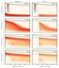 |
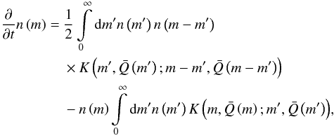
Fig. 4 Different snapshots of our fiducial model. Shown are the different distribution functions as defined by Eqs. (43) at 10 000 yr, 100 000 yr, 500 000 yr, and at 1 Myr. The solid line denotes the particle sizes with Stokes number unity, The dashed line is an analytical estimation of the drift barrier. The dotted line encompasses a region outside of the ice line that is free of small particles. |
Figure 4 shows different snapshots of the size evolution in our fiducial model. Plotted are the following distribution functions:  (43)The solid line denotes the particles with a Stokes number of unity. The dashed line is an analytical estimate of the maximum drift-limited particle size as given by Birnstiel et al. (2011). At first, the particle growth is most effective in the inner regions of the disk because of the larger collission rates of the particles. The particle growth is later hindered by radial drift. In the snapshots at 500 000 yr and 1 Myr, a region from the ice line at 47 AU outwards can be seen where there are no small particles (dotted line). Because of the re-condensation of CO, these particles grow in size. The distribution functions σ are therefore compressed towards larger sizes leading to the darker spot at intermediate particle sizes in the μm range. The total number density of particles has no discontinuity at the ice line.
To investigate the typical particle size  that carries most of the CO ice mass and the typical particle size
  that transports most of the CO ice, we define the following quantities:
  is the average particle size weighted by the CO dust distribution and is the average particle size weighted by the CO ice flux. Both quantities are plotted in Fig. 5. It can be seen by comparing Fig. 5 with Fig. 4 that is always close to the maximum particle size. Furthermore, is always close to the particle size that is responsible for the ice flux on the particles in the disk.
3.2. Transport of CO in the dust phase
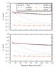 |
Fig. 5 Typical particle size |
Figure 6 shows the excess in total dust surface density compared to a model without CO, the dust-to-gas ratio and the ice-to-dust ratio for different values of the initial gas-to-CO ratio fg2CO at different times in the simulation. We used values for fg2CO of 70, 700 (fiducial model), and 7000, which correspond to CO abundances of 10-3, 10-4, and 10-5. For guidance, the horizontal lines mark the values for the quantities one would expect outside the ice line simply from the initial conditions. The excess is defined as Σi/ Σ0−1, where Σi is the total dust surface density in the models of the different CO abundances and Σ0 is the total dust surface density in the model without CO. The initial value of the excess outside the ice line is fg2d/fg2CO. The initial value of the gas-to-dust ratio is 1 /fg2d + 1 /fg2CO. The ice-to-dust ratio compares the surface density of CO ice to the total dust surface density. Its initial value is fg2d/ (fg2d + fg2CO).
It can be seen that the closer the CO ice line is to the star, the higher the CO abundance is. Further, the more CO there is in the system, the more saturated the evaporation/condensation is, causing the ice line to be pushed inwards. This varies the position of the CO ice line in these models from approximately 40 AU to 50 AU, initially.
The left panels show the excess compared to a model without CO. Notably, the excess inside the ice line is nonzero in all cases, meaning the total surface density is still higher than in the comparison model without CO. Because of the larger CO-coated particles in the models with CO, and therefore the more effective drift, the dust surface density is enhanced inside the ice line. This is especially visible in the high abundance model. In some models, the excess at the ice line can be a few times larger than one would expect from the initial values. This is due to accumulation and re-distribution of CO at the ice line.
In general, the dust-to-gas ratio decreases with time. The dust surface density decreases while the gas density remains approximately constant over time, as discussed later. The dust-to-gas ratio decreases from inside out because the particle growth is most efficient in the inner parts of the disk, meaning the particles start to drift earlier than outside. The dust-to-gas ratio is increased at the location of the ice line. This is due to two effects: first, as the particles drift through the ice line, they shrink because of evaporation, making drift less efficient and therefore leading to a “traffic jam”, and second, the backwards-diffusing and re-condensing CO vapor increases the ice surface density outside the ice line.
This effect can also be seen in the ice-to-dust ratio. At 1 Myr, the ice-to-dust ratio is enhanced above the initial value even at radii larger than 70 AU depending on the model.
3.3. Transport of CO in the gas phase
 |
Fig. 6 Excess of total dust surface density compared to a model without CO, the dust-to-gas ratio and the ice-to-dust ratio at different times for initial gas-to-CO ratios of 70 (dotted red line), 700 (fiducial model, solid green line) and 7000 (dashed blue line). The horizontal gray lines are the respective quantities one would expect from the initial conditions outside the ice line. |
CO is radially transported in the disk via three mechanisms: viscous accretion and diffusion in the gas phase and frozen-out as ice on drifting particles. As, outside of the ice line, most of the CO is frozen-out on particles, the dominant radial transport mechanism there is particle drift. Inside the ice line, on the other hand, all of the CO exists in the gas phase and is radially transported by viscous accretion and diffusion.
This means that transport of CO through the ice line from the outside into the inner part of the disk happens on drifting dust particles, while transport from the inside to the outside takes place in the gas phase. The efficiency of viscous accretion is highly dependent on the viscosity parameter α while the drift velocity of particles depends on their size and is only indirectly related to α through the dust growth.
Particles are drifting through the ice line and deposit their CO as vapor there. The strength of α determines how rapidly this CO vapor is diffused from there. This is shown in Fig. 7 where we compared our fiducial model, with α = 10-3, with a low-viscosity model of α = 10-4 and a high-viscocity model of α = 10-2 at the time of 1 Myr. Plotted is the ratio of the CO gas surface density ΣCO to the total gas surface density Σgas at the region of the ice line. Also plotted is the ratio of to Σgas. The ice line is therefore defined as the position where the CO gas phase abundance approaches the level set by the equilibrium density (dashed black line). This can happen anywhere from 39 to 49 AU approximately, depending on the assumed viscosity and consequently the CO gas abundance. The lower the viscosity, the more efficient the accumulation of gas, pushing the ice line closer to the star.
Even though the temperature structure is the same for all three models, there is still a difference in the location of the ice line. The reason for this is that evaporation/condensation not only depends on the temperature but also on the partial pressure of CO, as seen in Eq. (28). The partial pressure depends on the amount of vaporized CO at a given location and on the temperature (cf. Eq. (32)). This means that, in principle, any system can be in saturation (ie., Eq. (28) equals zero) for any temperature if the density is high enough. In our fiducial model, at 1 Myr, (green solid line in Fig. 7) this happens at ~47 AU where the temperature is ~22 K.
In the beginning of the simulations, the ice lines of the different models were at the same position. As soon as the particles start to grow, they drift inwards, cross the ice line, and deposit their CO there. Depending on the efficiencies of accretion and mixing, the system can become saturated at the ice line if more CO vapor gets deposited there by drifting particles than can be transported away in the gas phase. If that is the case, then the ice line moves inwards because the particles can only evaporate when they are in a region where the system is not in saturation. Therefore, the ice line in the low-α models is closer to the star than the ice line in the fiducial model. As mentioned above, this inward motion of the ice line is entirely due to non-thermal effects, as we consider a time invariant temperature structure. Should the midplane temperature change, due to changes in disc flaring, for example, this would have a more noticeable effect on the ice line location as shown in Panić & Min (2017).
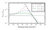 |
Fig. 7 Ratio of CO gas surface density to total gas surface density after 1 Myr in the region of the ice line. Shown are the fiducial model with α = 10-3 (solid green line), a low-viscosity model with α = 10-4 (dashed blue), and a high-viscosity model with α = 10-2 (dotted purple). The ratio of |

We also show, in Fig. 7, a model where we turned off the viscous evolution of the gas disk by not solving Eq. (7). This is equivalent to setting α = 0. In this case, all the CO vapor remains where it is evaporated, and this moves the ice line inwards to approximately 39 AU compared to the fiducial case at 47 AU. In the region just inside the ice line, the ratio ΣCO/ Σgas is largely increased compared to the initial ratio of 1 /fg2CO depending on the strength of viscosity. In the fiducial model, ΣCO/ Σgas is, in general, slightly increased in the inner part of the disk, since the transport of evaporated CO from the ice line to the inner disk is more effective here.
In the high viscosity case, the re-distribution of vapor is stronger than the recondensation onto the particles. Meaning, vapor from inside the ice line becomes diffused outwards faster than it can recondense onto the particles. This can be seen as the ratio of CO vapor to total gas is decoupled from the equilibrium evaporation line. In this case, no increase of CO vapor in the inner disk can be seen.
3.4. The influence of diffusion on the position of the ice line
By rewriting the Eq. (4) for viscous accretion, one can see that it consists of an advective and a diffusive term with a diffusivity D = 3ν, as can be seen in Eq. (7). By introducing the Schmidt number Sc = ν/D, we disentangled the advective and diffusive terms. The Schmidt number compares the strength of angular momentum transport to pure mass transport. To investigate the influence of the diffusivity on the transport of CO, we performed simulations where we kept the viscosity, as in the fiducial model, at α = 10-3, and changed the diffusivity by choosing different Schmidt numbers.
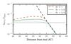 |
Fig. 8 Dependency of the ratio of CO vapor surface density to total gas surface density on the Schmidt number at 1 Myr. The fiducial model is identical to the model with Sc = 1/3 (green solid line). The dashed black line represents the ratio of |
The result is shown in Fig. 8. The green models in Figs. 7 and 8 are the fiducial model and are therefore identical. It can be seen that the diffusivity D is relevant for distributing the CO in the gas disk; it smears out concentration gradients. With lower diffusivities (higher Schmidt numbers), the pile-up of CO gas just inside the ice line gets larger because it cannot be transported rapidly enough as it gets deposited there. The ice line is therefore shifted slightly to the inside of the disk for models with higher Schmidt numbers.
One possibility to trap particles is to assume a pressure bump. The dust particles drift in the direction of the pressure gradient (cf. Eq. (17)). Kretke & Lin (2007) proposed such a pressure bump at ice lines because of a sharp transition of the turbulent viscosity parameter α at the ice line. In our model, we do not change α at the ice line. The pressure bumps we could create are therefore only due to evaporation of CO on inward-drifting particles, but to create such a pressure bump only by depositing CO gas is rather unrealistic since one would need to increase the CO gas surface density by a factor larger than fg2CO.
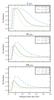 |
Fig. 9 Distribution of Q according to R for different silicate core sizes asil and different values of α = 10-4 (dotted red line), α = 10-3 (fiducial, solid green line) and α = 10-2 (dashed blue line) after 1 Myr. |
Figure 9 shows the distribution of ice along the different particle sizes dependent on α. For high-viscosity cases, the CO ice gets distributed as far out as 90 AU for small particles. In the low-viscosity case, the CO ice region is restricted up to 60 AU. Also, the higher the viscosity, the farther out the ice line. With high α (and therefore, via the Schmidt number, also high D), CO vapor cannot be accumulated at the ice line. This prevents any saturation effect.
4. Discussion
4.1. The CO surface density and ice line position
In the previous section, we showed that ΣCO, the vapor density of CO, approximately follows the equilibrium vapor density , as long as there is enough CO in the disk. If the evaporation/condensation timescales are shorter than the dynamical time scales of the system, the CO exactly follows the equilibrium density; if the evaporation/condensation timescales are longer than the dynamical timescales, it can decouple from the equilibrium vapor density. To first order, one can therefore approximate the CO vapor surface density in the whole disk with the equation ![Mathematical equation: \begin{equation} \Sigma_\mathrm{CO} = \min \left[ \frac{1}{f_\mathrm{g2CO}} \Sigma_\mathrm{gas},\; \Sigma_\mathrm{CO}^\mathrm{eq} \right]. \label{eqnSigmaCOApprox} \end{equation}](/articles/aa/full_html/2017/04/aa29041-16/aa29041-16-eq184.png) (46)Outside the ice line, the CO surface density is equal to
(46)Outside the ice line, the CO surface density is equal to  ; inside the ice line it is approximated by using the total surface density and the initial gas-to-CO ratio. Although, one should note that in Figs. 7 and 8, the ratio of ΣCO/ Σgas can be significantly increased just inside the ice line, depending on the values of α and Sc.
The position of the ice line Rice is then defined as the point where the CO surface density joins the equilibrium density and can be approximated by equating:  (47)Piso et al. (2015) showed, by comparing the desorption time tdes of evaporating particles with their respective drift timescale tdrift, that the location of the ice line does not necessarily coincide with the location where the system gets out of saturation. When the particles drift faster than they evaporate (i.e., tdes/tdrift ≫ 1), the particles drift far past the ice line before they evaporate their ice, leading to icy particles inside the ice line.
 |
Fig. 10 Comparing the desorption time tdes with the drift timescale tdrist. If the ratio tdes/tdrift is larger than unity, the particles can drift past the ice line before they fully evaporate their ices. The vertical dashed line is the location of the ice line in our model. |
Figure 10 shows the ratio of the desorption time tdes to the drift timescale tdrift for our fiducial model. The desorption time is given by  (48)whereas the drift timescale is given by
  (49)By comparing Fig. 10 with Fig. 4, one can see that the particles at the location of the ice line have a size where this “smearing-out” begins to happen. Figure 11 shows the CO ice surface density after 1 Myr in our fiducial model. The ice line of the smaller particles is at approximately 47 AU, whereas the ice line for the largest particles is at approximately 45 AU.
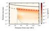 |
Fig. 11 CO ice surface density in our fiducial model after 1 Myr. The largest particles are just large enough such that their drift timescale is smaller than their desorption timescale leading to a “smearing-out” of the ice line. The solid line denotes the particle sizes with Stokes number of unity. The dashed line is the drift barrier. The dotted line encompasses an empty region outside the ice line. |
By using Eq. (46), one has to keep in mind that the values for ΣCO around the ice line and the position of the ice line itself highly depend on the transport properties of CO in the gas phase, that is, the viscosity ν and therefore the α turbulence parameter, and on the diffusivity D. If the transport mechanism of CO in the gas phase is not strong enough, that is, low α or low D, a pile-up of vaporized CO is created just inside the ice line. This brings the system into saturation even closer to the star and therefore shifts the ice line closer to the star. This can lead to differences in the position of the ice line of up to 10 AU and a change in temperature at the ice line from 21 K to 23 K. In an evolving disk, where the temperature profile is not fixed, the change in the position of the ice line can be even stronger due to changes in the midplane temperature (e.g., Panić & Min 2017). Also, in the high viscosity case, redistribution of CO can be strong enough for the vapor to be decoupled from the equilibrium vapor pressure.
By looking at Figs. 7 and 8, one can see that the CO vapor abundance in the inner part of the disk is significantly increased over to the canonical ISM value. This was also predicted by Cuzzi & Zahnle (2004, Regimes 1 and 2 therein). However, we cannot reproduce a depleted inner nebula as in Stevenson & Lunine (1988) and Cuzzi & Zahnle (2004, Regime 3) because we do not have any sink terms such as immobile planetesimals outside the ice line that can remove the vapor from the disk. Our particles on which the CO vapor re-condenses outside the ice line are still mobile and drift inwards through the ice line replenishing the CO vapor there. Only in the high-viscosity case does the inner disk become slightly depleted in CO vapor around the ice line due to the turbulent diffusion being effective enough to push the gas farther out against recondensation.
4.2. Particle growth at the ice line and detectability
We do not see an enhanced particle growth just outside the ice line; instead we see a depletion in surface density of dust inside the ice line. This depletion is entirely due to loss of CO ice mantles, thereby making the dust particles smaller and less massive. The particle surface density is dominated by particles close to their local drift barrier. CO vapor, that previously diffused backwards from inside the ice line and then recondensed on those particles outside the ice line, only increase their size and Stokes number, making them drift even more rapidly though the ice line. This drift barrier limits the sizes of the particles in our models to less than one centimeter at the CO ice line.
The depression in total dust surface density seen in Fig. 2 is therefore related to the amount of CO in the system. The radial jump in the total dust surface density is approximately given by the ratio  . If we assume that the loss of the CO ice mantle at the CO ice line does not cause any differences to the optical properties of the dust in the mm-wavelength regime, then the difference in the intensity by thermal continuum emission of the dust Sν is dominated by the difference in surface density of the dust. Using the optically thin approximation
 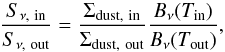 (50)where Bν(T) is the Planck function and in/out refers to locations shortly inside/outside the ice line. The dust densities are given by
 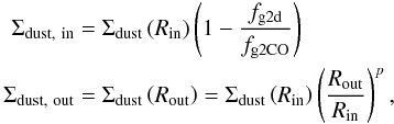 (51)by assuming a simple power law for the dust surface density
 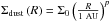 . This leads to
  (52)by assuming a canonical ISM value of fg2d/fg2CO = 1/7 (see e.g., Yamamoto et al. 1983) and Bν(Tin) /Bν(Tout) ≃ 1. To detect the effect of the CO evaporation and to quantify fg2d/fg2CO (under the assumption that no other process causes a bump at the ice line), it is clear that one needs to constrain p in the region beyond the ice line and measure Sν at Rice to S/N much greater than 7.
4.3. Influence of the particle size on the fragmentation velocity
Okuzumi et al. (2016) showed that a change in the fragmentation velocity due to sintered aggregates in the proximity of ice lines can produce rings in disks, as observed for example in the disk around HL Tau. Evaporation preferentially happens on convex surfaces, while condensation preferentially happens on concave surfaces. Close to the ice line, evaporation starts to happen on the convex surface of a monomer, while simultaneously, condensation can happen on the concave contact point (“neck”) of two connected monomers (Sirono 2011). This effect stiffens the neck making it harder for the monomers to roll around this contact point. Aggregates can absorb the impact energy of collisions by restructuring via rolling (Dominik & Tielens 1997). Sintering reduces the possibility of rolling leading to a breakup of the monomer connections and therefore a lower fragmentation velocity.
In contrast to that, the critical breaking velocity necessary to break up the connection of two monomers is inversely proportional to the monomer size  (cf. Dominik & Tielens 1997) leading to lower fragmentation velocities for aggregates with larger monomer sizes. We showed in Fig. 3 that our particles with a silicate core of 0.1 μm (the monomers) have an ice fraction of Q> 0.999 in the region outside the ice line. The monomer size in that region is therefore increased by a factor of at least 10 and the fragmentation velocity decreased by a factor of approximately 7. This could lead to enhanced fragmentation just outside ice lines and requires further investigation in upcoming works.
Possible improvements of the model
-
1.
Our model is one-dimensional and we only use surfacedensities in our calculations. This leads to errors inΣCO in our treatment of the evaporation/condensation described in Sect. 2.5. We underestimate ΣCO since we are neglecting the CO in the hot surface layers of the disk. However, since the disk’s atmosphere is small compared to its scale height, and its density is significantly smaller than the midplane density, this should not be a large effect.
-
2.
We do not take into account the vertical movement of dust particles. This movement could also influence the vertical distribution of CO gas. One could imagine that the CO gas condenses on small dust particles in the surface of the disk. These particles then sink more easily towards the midplane and remove CO vapor from the disk’s atmosphere. Or, vice versa, small CO-coated dust particles are pushed through the atmospheric ice line due to turbulence, depositing their CO as gas in the disk’s surface. This is a topic of further investigation.
-
3.
We also do not take into account the vertical diffusion of CO vapor and how this affects the local CO vapor pressure in the midplane. As particles grow, they settle to the midplane. When they drift inwards through the ice line, one would think that most of the CO vapor is set free close to the midplane and is not instantaneously in thermal equilibrium as we assume in our model.
-
4.
In our model we treat the particles as compact spheres, but Kataoka et al. (2013) showed that, through fractal growth, the particles can potentially overcome the drift barrier. The reason for this is that fluffy aggregates have larger cross-sections than compact aggregates of the same mass. This decreases the growth timescales of the particles, making the growth of the particles more efficient and potentially making it possible to overcome the drift barrier.
-
5.
Treating particles as compact spheres and not as fluffy aggregates could lead to an artificial “non-fragmentation” by evaporation, since we combine the silicate mass of the particle in one particle core after evaporation of the CO instead of creating many small particles as Aumatell & Wurm (2011) suggested.
-
6.
Including fragmentation and looking at the inner disk can potentially change some results. In general, the particle size in the inner parts of the nebula is fragmentation limited instead of drift limited, as in the outer disk. Therefore, the particle dynamics and distributions change, which can have effects on the various volatile re-distribution mechanisms discussed in this paper.
5. Conclusions and outlook
We developed a model for dust growth with a volatile species including particle drift and diffusion, evaporation and condensation of the volatiles, and viscous evolution of the gas. We do not find any enhanced particle growth by re-condensation just outside the ice line, since the particles there are already close to their drift barrier. Due to particle drift through the ice line, evaporation, diffusion and re-condensation on particles outside the ice line, we find a dust surface density enhancement at the ice line that could be observable at the CO ice line. The vapor that gets deposited at the ice line by inwards-drifting particles can push the ice line closer to the star. If the efficiency of re-distribution of vapor in the disk is low, then the vapor accumulates at the ice line, bringing the system into saturation and therefore preventing evaporation. The location of the ice line itself does depend on disk parameters such as temperature, volatile abundance, viscosity, or diffusivity. Furthermore, different particle sizes can have, in general, different locations at which they fully evaporate their volatile species. The increase in monomer size just outside the ice line could lead to fragmentation, exactly as proposed for sintering.
Our model is not restricted to CO. By using the analogous parameters for water ice, we can transfer the simulation to the water ice line in the inner disk. Here, one has to take into account that the collisional properties of water-ice-coated particles and purely silicate particles differ tremendously (e.g., Blum & Wurm 2008; Güttler et al. 2010). For ice-free particles, fragmentation plays an important role and has to be taken into account for particles crossing the ice line. Furthermore, the water ice line is at locations in the disk where viscous heating is important and has to be taken into account. The question of the location and distribution of H2O has an important role in astrophysics and planetary sciences. Whether the Earth formed dry, that is, inside the water ice line, or in a region outside the ice line remains to be determined. If the Earth formed dry, the origin of the Earth’s water is unclear. If it formed wet, the relatively small amount of water observed on Earth is curious. By transforming our model to water ice and implementing fragmentation, we will try to come closer to elucidating these subjects in future work.
Acknowledgments
S.M.S. has been supported by the Deutsche Forschungsgemeinschaft Schwerpunktprogramm (DFG SPP 1385) “The First 10 Million Years of the Solar System – a Planetary Materials Approach”. S.M.S. gratefully acknowledges support through the PUC-HD Graduate Student Exchange Fellowship, which is part of the academic exchange program between the Institute of Astrophysics of the Pontificia Universidad Católica (IA-PUC) and the Center for Astrophysics at the University of Heidelberg (ZAH), financed by the German Academic Exchange Service (DAAD). The work of O.P. is supported by the European Union through the grant number 279973, and by the Royal Society Dorothy Hodgkin Fellowship, number 140243.
References
- Ali-Dib, M., Mousis, O., Petit, J.-M., & Lunine, J. I. 2014, ApJ, 793, 9 [NASA ADS] [CrossRef] [Google Scholar]
- Aumatell, G., & Wurm, G. 2011, MNRAS, 418, L1 [NASA ADS] [CrossRef] [Google Scholar]
- Bai, X.-N., & Stone, J. M. 2010, ApJ, 722, 1437 [NASA ADS] [CrossRef] [Google Scholar]
- Birnstiel, T., Dullemond, C. P., & Brauer, F. 2010, A&A, 513, A79 [NASA ADS] [CrossRef] [EDP Sciences] [Google Scholar]
- Birnstiel, T., Ormel, C. W., & Dullemond, C. P. 2011, A&A, 525, A11 [NASA ADS] [CrossRef] [EDP Sciences] [Google Scholar]
- Blum, J., & Wurm, G. 2008, ARA&A, 46, 21 [NASA ADS] [CrossRef] [EDP Sciences] [Google Scholar]
- Brauer, F., Dullemond, C. P., & Henning, T. 2008, A&A, 480, 859 [NASA ADS] [CrossRef] [EDP Sciences] [Google Scholar]
- Cuzzi, J. N., & Zahnle, K. J. 2004, ApJ, 614, 490 [NASA ADS] [CrossRef] [Google Scholar]
- Dominik, C., & Tielens, A. G. G. M. 1997, ApJ, 480, 647 [NASA ADS] [CrossRef] [Google Scholar]
- Drążkowska, J., & Dullemond, C. P. 2014, A&A, 572, A78 [NASA ADS] [CrossRef] [EDP Sciences] [Google Scholar]
- Garaud, P., Meru, F., Galvagni, M., & Olczak, C. 2013, ApJ, 764, 146 [NASA ADS] [CrossRef] [Google Scholar]
- Gundlach, B., & Blum, J. 2015, ApJ, 798, 34 [NASA ADS] [CrossRef] [Google Scholar]
- Güttler, C., Blum, J., Zsom, A., Ormel, C. W., & Dullemond, C. P. 2010, A&A, 513, A56 [NASA ADS] [CrossRef] [EDP Sciences] [Google Scholar]
- Haisch, Jr., K. E., Lada, E. A., & Lada, C. J. 2001, ApJ, 553, L153 [NASA ADS] [CrossRef] [Google Scholar]
- Johansen, A., & Klahr, H. 2005, ApJ, 634, 1353 [NASA ADS] [CrossRef] [Google Scholar]
- Johansen, A., Oishi, J. S., Mac Low, M.-M., et al. 2007, Nature, 448, 1022 [Google Scholar]
- Kataoka, A., Tanaka, H., Okuzumi, S., & Wada, K. 2013, A&A, 557, L4 [NASA ADS] [CrossRef] [EDP Sciences] [Google Scholar]
- Kretke, K. A., & Lin, D. N. C. 2007, ApJ, 664, L55 [NASA ADS] [CrossRef] [Google Scholar]
- Kretke, K. A., Lin, D. N. C., & Turner, N. J. 2008, in IAU Symp. 249, eds. Y.-S. Sun, S. Ferraz-Mello, & J.-L. Zhou, 293 [Google Scholar]
- Leger, A., Jura, M., & Omont, A. 1985, A&A, 144, 147 [NASA ADS] [Google Scholar]
- Lynden-Bell, D., & Pringle, J. E. 1974, MNRAS, 168, 603 [NASA ADS] [CrossRef] [Google Scholar]
- Mathis, J. S., Rumpl, W., & Nordsieck, K. H. 1977, ApJ, 217, 425 [NASA ADS] [CrossRef] [Google Scholar]
- Nakamoto, T., & Nakagawa, Y. 1994, ApJ, 421, 640 [NASA ADS] [CrossRef] [Google Scholar]
- Öberg, K. I., Murray-Clay, R., & Bergin, E. A. 2011, ApJ, 743, L16 [NASA ADS] [CrossRef] [Google Scholar]
- Okuzumi, S., Momose, M., Sirono, S.-I., Kobayashi, H., & Tanaka, H. 2016, ApJ, 821, 82 [NASA ADS] [CrossRef] [Google Scholar]
- Okuzumi, S., Tanaka, H., & Sakagami, M.-A. 2009, ApJ, 707, 1247 [NASA ADS] [CrossRef] [Google Scholar]
- Panić, O., & Min, M. 2017, MNRAS, submitted [Google Scholar]
- Pavlyuchenkov, Y., & Dullemond, C. P. 2007, A&A, 471, 833 [NASA ADS] [CrossRef] [EDP Sciences] [Google Scholar]
- Piso, A.-M. A., Öberg, K. I., Birnstiel, T., & Murray-Clay, R. A. 2015, ApJ, 815, 109 [NASA ADS] [CrossRef] [EDP Sciences] [Google Scholar]
- Qi, C., Öberg, K. I., Andrews, S. M., et al. 2015, ApJ, 813, 128 [NASA ADS] [CrossRef] [Google Scholar]
- Ros, K., & Johansen, A. 2013, A&A, 552, A137 [NASA ADS] [CrossRef] [EDP Sciences] [Google Scholar]
- Schräpler, R., & Henning, T. 2004, ApJ, 614, 960 [NASA ADS] [CrossRef] [Google Scholar]
- Shakura, N. I., & Sunyaev, R. A. 1973, A&A, 24, 337 [NASA ADS] [Google Scholar]
- Sirono, S.-i. 2011, ApJ, 735, 131 [NASA ADS] [CrossRef] [Google Scholar]
- Stevenson, D. J., & Lunine, J. I. 1988, Icarus, 75, 146 [NASA ADS] [CrossRef] [Google Scholar]
- Wada, K., Tanaka, H., Suyama, T., Kimura, H., & Yamamoto, T. 2009, ApJ, 702, 1490 [NASA ADS] [CrossRef] [Google Scholar]
- Weidenschilling, S. J. 1977, MNRAS, 180, 57 [NASA ADS] [CrossRef] [Google Scholar]
- Windmark, F., Birnstiel, T., Ormel, C. W., & Dullemond, C. P. 2012, A&A, 544, L16 [NASA ADS] [CrossRef] [EDP Sciences] [Google Scholar]
- Yamamoto, T., Nakagawa, N., & Fukui, Y. 1983, A&A, 122, 171 [NASA ADS] [Google Scholar]
- Youdin, A. N., & Goodman, J. 2005, ApJ, 620, 459 [NASA ADS] [CrossRef] [Google Scholar]
- Youdin, A. N., & Shu, F. H. 2002, ApJ, 580, 494 [NASA ADS] [CrossRef] [Google Scholar]
Appendix A: Modified Podolak algorithm for Q
Brauer et al. (2008) described, in their Appendix A, the difficulties of numerically solving the discrete Smoluchowski equation for coagulation on a logarithmically spaced mass grid. They present a method for circumventing these problems. This method has to be modified for the Q parameter used in this work.
We will shortly repeat the formalism of Brauer et al. (2008). For further details we refer to that paper.
By coagulating two particles on a logarithmic mass grid, the resulting particle’s mass will not be exactly on a grid point. Therefore, its mass has to be split between two adjacent grid points. Let us assume the collision rate Rij of particles with masses mi and mj is given by  (A.1)where Ni is the number density of particle species i, and Kij is the coagulation Kernel of mass bins i and j. The resulting particle mass of these collisions is m = mi + mj, which lies in between the two mass grid points mm and mn such that mm<m<mn. The change in number density of mass bin k is then given by
  (A.2)with
  (A.3)and
  (A.4)This guarantees that the collision rates are split between two adjacent grid points with strict mass conservation, which can be easily calculated.
Another problem arises if particles coagulate, whose masses differ by more than 15 orders of magnitude. Standard double precision variables have accuracies up to 15 digits. In that case, for a computer using double precision variables, a sticking collision of two particles with masses mi and mj would lead to a particle with mass m = mi + mj = mj when mj is the larger particle, meaning many collisions of very small particles with a very large particle would lead to no growth at all, which is solely a numerical effect.
Brauer et al. (2008) avoided this by re-sorting sums. They came to the following equation:  (A.5)where the matrix M is given by
  (A.6)where δ is the Kronecker delta and Θ the Heaviside step function. The matrices D and E are given by
  (A.7)and
 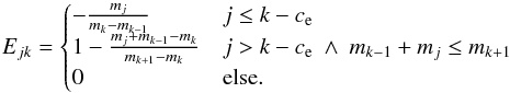 (A.8)The integer number ce is defined in a way that the inequality,
 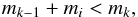 (A.9)is satisfied for every i ≤ k−ce. In that way, some equal sized terms cancel out in the sums and inaccuracies resulting from the limited accuracy of the double precision variables can be avoided. Unfortunately, by introducing the Q parameter, these terms do not exactly cancel out in the coagulation equation for NQi ≡ Ni·Qi. We have to modify the equations here to get to
 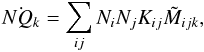 (A.10)with the matrix
  that can be expressed in terms of M as
 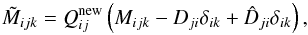 (A.11)and
  (A.12)
 is the new Q-value of the particle that resulted from the collision of particle i with particle j.
All Tables
All Figures
|
Fig. 1 Gas surface densities of the fiducial model after 1 Myr. Shown are the total gas surface density (solid black line) and the surface density of gaseous CO (dashed green line). The dotted blue line is the equilibrium surface density of CO given by Eq. (32). The location where the CO surface density detaches from the equilibrium CO surface density is called the ice line. |
| In the text | |
|
Fig. 2 Dust surface densities of different dust sizes at the CO ice line after 1 Myr. Shown are the total surface density (solid gray line), millimeter-sized (dotted blue line), sub-millimeter-sized (dashed red line), and sub-micrometer-sized (dash-dotted green line) particles. The vertical dashed line marks the location of the CO ice line. |
| In the text | |
|
Fig. 3 CO ice fraction Q of particles with different silicate core sizes depending on their radial position in the disk after 1 Myr. |
| In the text | |
|
Fig. 4 Different snapshots of our fiducial model. Shown are the different distribution functions as defined by Eqs. (43) at 10 000 yr, 100 000 yr, 500 000 yr, and at 1 Myr. The solid line denotes the particle sizes with Stokes number unity, The dashed line is an analytical estimation of the drift barrier. The dotted line encompasses a region outside of the ice line that is free of small particles. |
| In the text | |
|
Fig. 5 Typical particle size |
| In the text | |
|
Fig. 6 Excess of total dust surface density compared to a model without CO, the dust-to-gas ratio and the ice-to-dust ratio at different times for initial gas-to-CO ratios of 70 (dotted red line), 700 (fiducial model, solid green line) and 7000 (dashed blue line). The horizontal gray lines are the respective quantities one would expect from the initial conditions outside the ice line. |
| In the text | |
|
Fig. 7 Ratio of CO gas surface density to total gas surface density after 1 Myr in the region of the ice line. Shown are the fiducial model with α = 10-3 (solid green line), a low-viscosity model with α = 10-4 (dashed blue), and a high-viscosity model with α = 10-2 (dotted purple). The ratio of |
| In the text | |
|
Fig. 8 Dependency of the ratio of CO vapor surface density to total gas surface density on the Schmidt number at 1 Myr. The fiducial model is identical to the model with Sc = 1/3 (green solid line). The dashed black line represents the ratio of |
| In the text | |
|
Fig. 9 Distribution of Q according to R for different silicate core sizes asil and different values of α = 10-4 (dotted red line), α = 10-3 (fiducial, solid green line) and α = 10-2 (dashed blue line) after 1 Myr. |
| In the text | |
|
Fig. 10 Comparing the desorption time tdes with the drift timescale tdrist. If the ratio tdes/tdrift is larger than unity, the particles can drift past the ice line before they fully evaporate their ices. The vertical dashed line is the location of the ice line in our model. |
| In the text | |
|
Fig. 11 CO ice surface density in our fiducial model after 1 Myr. The largest particles are just large enough such that their drift timescale is smaller than their desorption timescale leading to a “smearing-out” of the ice line. The solid line denotes the particle sizes with Stokes number of unity. The dashed line is the drift barrier. The dotted line encompasses an empty region outside the ice line. |
| In the text | |
Current usage metrics show cumulative count of Article Views (full-text article views including HTML views, PDF and ePub downloads, according to the available data) and Abstracts Views on Vision4Press platform.
Data correspond to usage on the plateform after 2015. The current usage metrics is available 48-96 hours after online publication and is updated daily on week days.
Initial download of the metrics may take a while.