| Issue |
A&A
Volume 600, April 2017
|
|
|---|---|---|
| Article Number | A55 | |
| Number of page(s) | 17 | |
| Section | Stellar structure and evolution | |
| DOI | https://doi.org/10.1051/0004-6361/201527902 | |
| Published online | 29 March 2017 | |
A refined analysis of the low-mass eclipsing binary system T-Cyg1-12664⋆
1 Astrophysics Department, Universidad de La Laguna, 38205 La Laguna, Tenerife, Spain
2 Centro de Estudios de Física del Cosmos de Aragón, Plaza San Juan 1, 44001 Teruel, Spain
e-mail: This email address is being protected from spambots. You need JavaScript enabled to view it.
3 Harvard-Smithsonian Center for Astrophysics, 60 Garden Street, Cambridge, MA 02138, USA
4 Instituto de Astrofísica de Canarias, 38200 La Laguna, Tenerife, Spain
5 SETI Institute, 189 Bernardo Ave, Mountain View, CA 94043, USA
Received: 4 December 2015
Accepted: 11 January 2017
Abstract
Context. The observational mass-radius relation of main sequence stars with masses between ~0.3 and 1.0 M⊙ reveals deviations between the stellar radii predicted by models and the observed radii of stars in detached binaries.
Aims. We generate an accurate physical model of the low-mass eclipsing binary T-Cyg1-12664 in the Kepler mission field to measure the physical parameters of its components and to compare them with the prediction of theoretical stellar evolution models.
Methods. We analyze the Kepler mission light curve of T-Cyg1-12664 to accurately measure the times and phases of the primary and secondary eclipse. In addition, we measure the rotational period of the primary component by analyzing the out-of-eclipse oscillations that are due to spots. We accurately constrain the effective temperature of the system using ground-based absolute photometry in B, V, RC, and IC. We also obtain and analyze VRCIC differential light curves to measure the eccentricity and the orbital inclination of the system, and a precise Teff ratio. From the joint analysis of new radial velocities and those in the literature we measure the individual masses of the stars. Finally, we use the PHOEBE code to generate a physical model of the system.
Results. T-Cyg1-12664 is a low eccentricity system, located d = 360 ± 22 pc away from us, with an orbital period of P = 4.1287955(4) days, and an orbital inclination i = 86.969 ± 0.056 degrees. It is composed of two very different stars with an active G6 primary with Teff1 = 5560 ± 160 K, M1 = 0.680 ± 0.045 M⊙, R1 = 0.799 ± 0.017 R⊙, and a M3V secondary star with Teff2 = 3460 ± 210 K, M2 = 0.376 ± 0.017 M⊙, and R2 = 0.3475 ± 0.0081 R⊙.
Conclusions. The primary star is an oversized and spotted active star, hotter than the stars in its mass range. The secondary is a cool star near the mass boundary for fully convective stars (M ~ 0.35 M⊙), whose parameters appear to be in agreement with low-mass stellar model.
Key words: stars: fundamental parameters / stars: low-mass / binaries: eclipsing / binaries: spectroscopic
Full Tables 1–3 and 10 are only available at the CDS via anonymous ftp to cdsarc.u-strasbg.fr (130.79.128.5) or via http://cdsarc.u-strasbg.fr/viz-bin/qcat?J/A+A/600/A55
© ESO, 2017
1. Introduction
T-Cyg1-12664 (KIC 10935310, 2MASS J19513982+4819553) is a low-mass detached eclipsing binary (LMDEB) at α = 19:51:39.824, δ = +48:19:55.38 (J2000.0). It was first discovered in the T-Cyg1 field of the Trans-Atlantic Exoplanet Survey (TrES; Alonso et al. 2004), and it is also in the Kepler mission field of view. Because of its intermediate orbital period (~4.129 d) and low mass ratio (q≃ 0.55), this system can serve as a benchmark for low-mass (M < 1 M⊙) stellar evolution models that have problems with the radii predicted for the stars.
The discovery and first analysis of T-Cyg1-12664 was reported by Devor et al. (2008a) and Devor (2008) using TrES photometric data. They obtained a small number of radial velocity (RV) observations, including only one RV measurement of the faint secondary star. Their RV measurements show that the period initially identified in the TrES photometry (8.26 days) was in fact of 4.129 days, and a secondary eclipse would be buried in the TrES data. From that first analysis Devor (2008) estimate masses of about 0.62 M⊙ and 0.32 M⊙ for the primary and secondary. Çakırlı et al. (2013) reanalyzed this system using new RV measurements, the high precision Kepler mission light curves and R-band ground-based photometry and obtained the following values for the masses and radii of the stars: M1 = 0.680 ± 0.021 M⊙, R1 = 0.613 ± 0.007 R⊙; and M2 = 0.341 ± 0.012 M⊙, R2 = 0.897 ± 0.012 R⊙. In their study, while the radius of the primary is consistent with main sequence low-mass stellar models, the radius of the secondary defies interpretation as a main-sequence star.
After its publication in Devor et al. (2008a), we included T-Cyg1-12664 in our observing program to refine the physical parameters of several LMDEBs. Here we present a thorough analysis of the system based on the Kepler photometry, new ground-based multiband photometry and RV measurements, and a specific photometric calibration carried out to obtain unbiased colors and precise, photometry-based effective temperatures. The outline of this work is as follows. In Sects. 2 and 3 we describe the Kepler and the ground-based RV and photometric observations. Section 4 describes a careful analysis of the system, including specific sections for a consistent photometric calibration, effective temperature, a careful treatment of the third light, and the orbital eccentricity. Finally, the absolute parameters and the distance of the system are computed in Sect. 6, with Sect. 6.3 devoted to comparing our results to the stellar models and previous results.
2. Light-curve observations
2.1. Kepler observations
T-Cyg1-12664 was observed by the Kepler spacecraft in Long Cadence mode from Q0 through Q17 (JD 2 454 953.54–JD 2 456 424.00). The observations were reduced using the Kepler mission pre-search data conditioning (PDC) pipeline (Jenkins et al. 2010), which produces high quality light curves like the ones illustrated in Figs. 1 and 2 for Q6. The instrumental systematics and spot-related activity in this star are readily visible in the Kepler light curves with out-of-eclipse variations deeper than the secondary eclipse.
We detrended the light curves from each quarter following a procedure similar to Slawson et al. (2011), by fitting Legendre polynomials to the out-of-eclipse data. The result for one quarter (Q6) is shown in Fig. 2. For T-Cyg1-12664 we had ephemeris information from preliminary works, so we could exclude the time intervals affected by eclipses, and it was not necessary to apply the iterative processes described in Slawson et al. (2011). Because of the effects of the spacecraft safe-modes and triggers, some quarters were divided in smaller intervals, but this detrending process was applied to all the Kepler mission photometry encompassing an interval of 1470 days. Typical Legendre polynomials orders were between 30 and 300, depending on the complexity of the variations and duration of the light-curves intervals. The result of this detrending is illustrated in the bottom panel of Fig. 2. This detrended light curve, provided in Table 1, was subsequently analyzed together with the ground-based photometry described in Sect. 2.2.
We note that this detrending process has the disadvantage of potentially removing information from the light curve, such as heating effects and proximity effects that are due to the shape of the stars. However, as we demonstrate in subsequent sections, these effects are negligible in T-Cyg1-12664, because of the large separation between the stars.
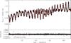 |
Fig. 1 Fit of an order 300 Legendre polynomial to the Kepler data in quarter 6. The upper panel shows the out-of-eclipse light curve and the fit (red line). The lower panel shows the residuals of the fit. |
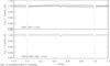 |
Fig. 2 Effect of the detrending over the phased light curve of Q6 quarter. Upper panel shows the raw light curve and lower panel shows the light curve after applying the Legendre polynomial fitted in Fig. 1. |
2.2. Ground-based observations
We observed T-Cyg1-12664 with the CAMELOT camera at the IAC80 telescope in Tenerife, Spain, in VRCIC bands, over 14 nights, between 2009-04-04 and 2010-10-01 UT (JD 2 454 936.6–JD 2 455 471.5), when eclipses occurred. We also requested a routinary observation program at the same telescope to sample out-of-eclipse phases. CAMELOT is equipped with a back-illuminated E2V 2048x2048 sensor with squared 13.5 μm pixels, which results in a plate scale of 0.̋304/pix and a 10.́4 × 10.́4 field of view.
Detrended Kepler light curve for T-Cyg1-12664.
Although CAMELOT has two readout channels, all the observations were made using one channel to avoid systematic effects between the object and the comparison stars. Exposure times ranged from 100 s to 180 s in V band, 65 s to 95 s in RC band, and 60 s to 90 s in IC band, depending on the seeing and the atmospheric transparency. Each night, we monitored T-Cyg1-12664 continuously over an altitude limit of 30 degrees (airmass ≤2) above the horizon. We also acquired bias frames and dome flats in all the filters at the beginning of each night.
We used standard reduction techniques, including bias substraction, flat-field correction, and alignment of all images to a common reference system, to process the frames. We analyzed the corrected frames using the phot aperture photometry package in IRAF and a custom differential photometry pipeline designed to deal with large sets of frames. The pipeline first performs aperture photometry for a set of preselected comparison stars and the target, for a range of aperture sizes. Using the flux within each aperture, the pipeline computes the signal-to-noise ratio (S/N) of the target using the CCD equation (Merline & Howell 1995, Eq. (25)), and selects the aperture radius that produces the maximum S/N. This aperture is then used to extract the flux of all the stars in that frame. This procedure accounts for seeing and transparency variations along the night. The CCD equation was also used to compute the formal errors in the photometry. We imposed a limit of 9 pixels to the maximum aperture radius to avoid contamination by nearby stars as is the case for T-Cyg1-12664 (see Sect. 4.5). The selected comparison stars proved to be stable during all the observing runs. We generated V, RC, and IC differential light curves of the target dividing its flux by the combined flux of all the comparison stars. Owing to the small field of view of the telescope no differential extinction effects were taken into account. Our VRCIC photometry (given in Table 2) includes seven primary and four secondary eclipses which, when added to those from the Kepler, Çakırlı et al. (2013) and TrES photometry, enable us to improve the period of the system and search for period variations.
IAC80 differential photometry for T-Cyg1-12664.
3. Radial velocity observations
We observed T-Cyg1-12664 as part of a larger program to produce accurate radial velocity curves of low-mass binaries (see Coughlin 2012). We collected radial velocity observations over two seasons (June–December 2010 and May–September 2011), with the Dual Imaging Spectrograph (DIS) on the 3.5-m at Apache Point Observatory and the R-C Spectrograph on the 4-m at Kitt Peak National Observatory (KPNO). With DIS we observed using its red channel with the R1200 grating, which gives a resolution of 0.58 Å per pixel, or R≈ 10 000. The wavelength range was set to ~5900–7100 Å for the first observing season, and ~5700–6800 Å for the second. For the R-C Spectrograph, we used the KPC-24 grating in second order, resulting in a resolution of 0.53 Å per pixel, or R≈ 10 000, with the wavelength range set to ~5700–6750 Å. We collected a total of 31 individual spectra for T-Cyg1-12664, in addition to bias, dark, and flatfield calibration frames. We also collected HeNeAr lamp frames before or after each target observation to use as wavelength calibrations.
All raw frames were bias, dark, and flat-field corrected. For the DIS observations, Col. 1023 is a dead column, and thus we replaced those values by a linear interpolation between the two neighboring columns. We also removed cosmic rays from all frames using a Laplacian edge algorithm implemented in the lacos_spec IRAF package (see van Dokkum 2001). Finally, we extracted one-dimensional spectra from each image, including sky background substraction, using the IRAF package apall. After wavelength calibration, all science spectra were flattened and normalized by fitting a 20-piece cubic spline fit over ten iterations, during which points 3σ above the fit or 1.5σ below the fit were rejected. For each spectrum, we calculated the barycentric Julian date in terrestrial time, BJD(TT), and corrected them to the reference frame of the solar system barycenter using the IRAF task bcvcorr.
For all binaries we attempted to extract the radial velocity of each star in each frame, V1,j and V2,j, where 1 and 2 denote the primary and secondary stars, and j is the frame number, using a new exploratory method: instead of using cross-correlations, we directly fit reference spectra to each observed spectrum via a traditional standard deviation minimization, which is equivalent to minimizing χ2, assuming all observed points have equal errors. Specifically, for each observed spectrum, we fit for the velocity of each reference spectra, as well as for their luminosity ratio, α = L1/L2, for a total of three free parameters. During the fitting, the original observed spectrum is never changed, and thus it can have any arbitrary number and distribution of wavelength and flux value pairs. Given a total of M observed spectra, each with Nj points, taken at times tj, we want to find the values of V1,j, V2,j, and α at each tj, that minimize the function 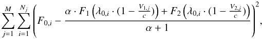 (1)where F0,i is the flux of an observed spectrum at a given wavelength, λ0,i, F1(λ), and F2(λ) are the fluxes of reference stars 1 and 2 at a given wavelength, and c is the speed of light. We determine F1(λ) and F2(λ) by cubic splines interpolation of the original reference spectra.
For reference spectra, we used the normalized (flattened) synthetic spectra from Munari et al. (2005). The Munari et al. (2005) grid we used covers models with 3500 ≥Teff≥ 10 000 in steps of 250 K, 0.0 ≥log g≥ 5.0 in steps of 0.5 dex, −2.5 ≥ [M/H] ≥ 0.5 in steps of 0.5 dex, and 0 ≥Vrot≥ 100 km s-1 in steps of 10 km s-1. To ensure that we found the global minimum in both selected reference spectra and their velocities, we performed a global grid search looping over all possible combinations of α, V1,j, V2,j, T1, T2, using a common [M/H] for both reference spectra, and log g and Vrot for each reference star. We compared the radial velocities found by this method with those obtained using the well-tested TODCOR code (Zucker & Mazeh 1994), and find consistent results for all the binaries in our program.
The errors in the derived radial velocities were computed using a bootstrapping re-sampling method iterated over 10 000 times. The adopted errors correspond to the 1σ confidence interval of the distribution of bootstrapping solutions. To estimate the errors in the derived temperatures, we used the spectroscopic quality-of-fit parameter (López-Morales & Bonanos 2008; Behr 2003), defined as 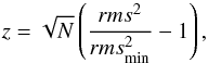 (2)where N is the number of data points, rms2 is the standard deviation of the fit under consideration, and
  is the best fit found. The z parameter is similar to a reduced χ2 in the absence of known errors on the individual points. By definition z = 0 at the best-fit, and the 1σ confidence interval corresponds to z = 1.
In the particular case of T-Cyg1-12664, the spectrum of the secondary is too weak, and we were unable to detect any significant radial velocity measurements for the secondary star over any reasonable parameter ranges. Thus, we treated the system as a single-lined binary by fixing the value of α to 9999 and only fitting for the parameters of the primary star V1,j, Teff1, [M/H], log g and Vrot. The resultant radial velocities are listed in Table 3. In addition, the best fit of the primary’s spectra to the grid of synthetic spectra gives a Teff = 5750 ± 250 K, log g = 4.5 ± 0.5, [ M / H ] =−0.5 ± 0.5 and vrsini = 40 ± 10 km s-1. This Teff is in agreement with the one obtained in Sect. 4.2 using photometric colors. The metallicity appears to be lower than the typical for stars near the Galactic plane (see Sect. 6.2), which would have near-solar metallicity. We attribute this result to the rather coarse sampling in metallicity of our models, and therefore adopt solar metallicity for this system in the remaining analysis.
We note that, although this χ2 minimization technique yields values of the radial velocities and other stellar parameters consistent with those obtained via other methods in the case of T-Cyg1-12664, the technique can be prone to systematics introduced by the presence of correlated noise or not well modeled spectral instrumental profiles, especially in the case of low S/N spectra. It is therefore advisable to have results checked against other methods like TODCOR.
Measured RV for the primary component in the T-Cyg1-12664 system.
4. Analysis of the system
4.1. Photometric calibration and colors
Photometry in several bands for T-Cyg1-12664 obtained from photometric catalogs.
In Table 4, we compile all the available photometry for T-Cyg1-12664 in public catalogs. We found inconsistencies between some of the passband magnitudes reported by different catalogs, e.g. the B and V magnitudes reported by the GSC and NOMAD catalogs disagree by 0.4–0.5 mag. The differences are too large to be explained by stellar activity, or even accounting for the depth of the eclipses (~0.20 in the Kepler band). We do not have an explanation for these discrepancies but, concerned about introducing large errors in the determination of parameters for this system, we proceeded to derive new, consistent colors.
We performed photometric calibrations of several objects, including T-Cyg1-12664, over two photometric nights in July and August 2012, during out-of-eclipse phases. We used the Trömso CCD Photometer in full frame mode (TCP, Östensen 2000; Östensen & Solheim 2000), at the IAC80 telescope (CAMELOT was not available at the time of these observations). The TCP is built around a Texas Instruments 1024 × 1024 CCD sensor and produces a 9.́6 field of view, with a plate scale of 0.̋537 pixel-1, at the IAC80’s focal plane.
We observed several Landolt standard fields (Landolt 2009), covering objects with a wide range of colors and airmasses, and using Johnson-Cousins B, V, RC, and IC filters. A log of the observations is shown in Table 5. We measured the flux of the standard stars via standard aperture photometry, using the IRAF package apphot, and adopting an aperture of 14′′ (a 13 pixel radius in the TCP images), to match the Landolt aperture widths.
Observed Landolt fields. The number of measurements is the global count for different air masses.
The extinction correction and transformation to the standard photometric system was performed simultaneously solving the set of equations 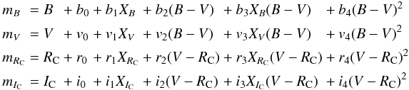 (3)
(3)
where the instrumental magnitudes appear on the left-hand side of the equations, the absolute magnitudes are denoted as B, V, RC, and IC, and the airmass values as X. The equations were solved using least-square techniques, and the resulting coefficients for each night are summarized in Table 6. The absolute magnitudes obtained for T-Cyg1-12664 as the average of the results for each night are summarized in Table 7. In that same table, we also list color indexes, including the near-infrared JHKS bands from 2MASS (Skrutskie et al. 2006).
Calibrated magnitudes and color indices for T-Cyg1 obtained from our photometric calibration.
Our B and V calibrated magnitudes are slightly fainter than the ones from Everett et al. (2012). We attribute the small differences (ΔB = 0.073, ΔV = 0.019), to stellar activity variations, as seen in Fig. 2. In the Kepler light curve these variations are of ΔmKp~ 0.022, which is very close to the variation we see in V band. The B−V index obtained by Everett et al. (2012) is 0.584 ± 0.030, which is slightly bluer than ours, mainly as a consequence of the difference in the B measurements.
4.2. Effective temperature
We derived the effective temperature of the system, Teff, using the empirical and model dependent, temperature–color relations listed in Table 8, our BVRCIC colors derived in Sect. 4.1, and the colors of the system published in 2MASS (Skrutskie et al. 2006), and the SDSS (Eisenstein et al. 2011). All those colors were measured outside of eclipses, which guarantees that no systematics were introduced by the dimming of the system during eclipse events. We still have the effect of stellar variability, which results in small variations of the color indexes. Those variations are accounted for in the Teff errors reported in Table 8.
Table 8 summarizes the values of the Teff derived using each temperature–color relation. We assumed negligible reddening in the direction of T-Cyg1-12664 when computing the colors but, in any case, the effect of the reddening over the distances involved will be smaller than the uncertainties in colors among the optical and IR bands, as a consequence of those colors being measured in different epochs and the intrinsic photometric variability of the system. The mean effective temperature adopted for the system, computed as the average of all the results in Table 8, is 5560 ± 160 K. This value is within 1σ of the value of Teff obtained from fitting our spectra in Sect. 3, and corresponds to a spectral type G6V, based on the tabulated values of Mamajek (2015). We adopted this result as the spectral type for the primary.
Mean effective temperature estimations resulting from our photometric calibration, 2MASS and SDSS photometry and our spectroscopy for T-Cyg1-12664.
Our Teff and spectral type of the primary do not agree with those derived by Devor (2008) and Çakırlı et al. (2013). In those studies the authors claim a K5V spectral type for the system and a mean Teff = 4320 ± 100 K. The main difference between their calculations and ours is their use of B and V magnitudes from the USNO catalog and GSC2.3.2, which we noticed in Sect. 4.1, are unreliable.
4.3. Spectral energy distribution
Given the difference between the spectral type obtained in this work and those in the literature, and as an additional check to the absolute photometry values derived in Sect. 4.1, we compared the optical and near-infrared colors measured for T-Cyg1-12664 to a Kurucz (1993) model template with Teff = 5500 K, log g = 4.5, and [M/H] = −0.5. The result is shown in Fig. 3, where the fit between the model and the observations produces an rms of 0.037 mag. We also repeated the same comparison with the calibrated photometry in Table 7 and a template model with the same metallicity and log g, but with Teff = 4250 K from Çakırlı et al. (2013). The best fit in this case produces an rms of 1.029 mag, with a clear systematic trend. Based on these results we conclude that the value of 5560 ± 160 K is a good estimate of the actual Teff for T-Cyg1-12664.
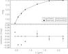 |
Fig. 3 Comparison between the absolute optical and 2MASS photometry with the synthetic photometry obtained for a Kurucz model with Teff = 5500 K, log g = 4.5, and [ M / H ] = −0.5. The uncertainties in the upper panel are smaller than the point sizes. |
4.4. Rotation and synchronicity parameter
The Kepler raw light curves of the system (see, for example, Fig. 2) reveals periodic photometric variations owing to spots, and with a period clearly different from that of the binary. In addition, and given the large differences in luminosity between the primary and secondary stars, we can attribute those photometric variations to spots on the primary star. Therefore, we can measure the rotation period of the primary, assuming that the spots rotate jointly with the photosphere. After normalizing each quarter of the Kepler raw light-curve, and removing the eclipses using the ephemeris equation of the system (see Sect. 4.6), we calculated Lomb-Scargle periodograms (Scargle 1982) for each normalized light curve. A prominent peak is seen in the periodogram from which we obtained rotation periods in a range between 3.840778 d and 4.250872 d. We attribute those variations to changes in the different spot configurations over the time span of the observations, and adopted a mean rotation period of Prot = 3.968 ± 0.091 d. That rotation period results in a synchronicity parameter F = ωrot/ωorb = 1.041 ± 0.024, using the period of the binary computed in Sect. 4.6. This value of F is too small to produce a significant deviation in the computed stellar radius and lets us assume that the primary star is rotationally synchronized with the orbital period. This Prot must be taken as an estimate, given that the star is not a rigid body with a well defined rotation period and, thus, this period depends on the latitude of the spots. For each of the two main spots in the Q6 interval, we measured the times tmin of each associated minima and plotted the difference T0−tmin versus the sequential number of each minima, with T0 defined as the time of a primary eclipse. We fit a straight line to each spot’s dataset and obtained slopes of 3.9659 ± 0.0092 d and 3.988 ± 0.010 d, which confirms the presence of differential rotation, as already revealed by the observed range of rotational periods. In addition, the spot with the lower rotation period is the one with lower latitude in the Q6-1 epoch (see Sect. 5.5), which suggests that the primary has solar-type differential rotation (see, for example, Reinhold & Arlt 2015; Lanza et al. 2014,and references therein).
4.5. Third light
T-Cyg1-12664 has an optical companion at a distance of 4.̋6 as pointed by Çakırlı et al. (2013), which is clearly seen in our images. We call this contaminant star T-Cyg1-C in the rest of the text. The aperture of our ground-based photometry avoids contamination by light from this star. Thus, our VRCIC differential photometry is free of this third light contribution. However, Kepler uses a photometric aperture of ~ 10−11 pix for T-Cyg1-12664 (roughly 3 × 3 pix), depending on the season, with a plate scale of 3′′98/pix. Given that this contaminant is not listed in the Kepler Input Catalog (KIC) it wouldn’t have been accounted for during Kepler’s third light calibration, and the Kepler light curve of T-Cyg1-12664 is affected by the flux of T-Cyg1-C.
To estimate the amount of third light in the Kepler passband, we had to rely on the flux of the contaminant in V, RC, and IC. We applied the photometric calibration performed on the night of 2012-07-26 to T-Cyg1-C, to obtain its magnitudes and colors listed in Table 9. From those colors we adopted Teff = 3761 ± 56 K for T-Cyg1-C, based on the calibrations of Cox (2000), Bessell (1991, 1979) and Lejeune et al. (1998). We didn’t use the B−V color index since their Teff is not consistent with the results of the other color indices and the B-band magnitude is too faint. Thus, we rely only on the colors that make use of V, RC, and IC photometry. From the obtained Teff, and assuming it is a main-sequence star, we adopted a spectral type of M0V for this star, using the tables in Mamajek (2015).
Fluxes and colors for T-Cyg1-C, the contaminant in the Kepler passband.
To estimate the Kepler band flux, Kp, for T-Cyg1-C we fit an spectral energy distribution (SED) using the observed colors and a Kurucz model spectrum with Teff = 3750 K and solar metallicity and obtain a geometric dilution parameter of (R∗/D)2 = (5.65 ± 0.14) × 10-22 over the integrated VRCIC bands (see Moro & Munari 2000). The uncertainty was computed performing Monte-Carlo fits over 100 iterations. We used the same Kurucz spectrum used in the synthetic SED, scaled by the computed dilution factor and integrated over the Kepler response function1 to estimate the contaminant flux due to T-Cyg1-C. The uncertainty was also computed with a Monte-Carlo analysis, as in the dilution factor case, and the obtained value is FKP = (5.88 ± 0.15) × 10-9 erg cm-2 s-1. For T-Cyg1-12664 we followed the same procedure but using a dilution factor of (R/D)2 = (2.7291 ± 0.0082) × 10-21, which results in a Kepler flux of FK = (2.5006 ± 0.0071) × 10-7 erg cm-2 s-1.
Using these fluxes for the binary and the contaminant, the third light ratio in the Kepler band results in  As a check of the feasibility of this result, we compared this value with the estimated amount of third light in the V, RC, and IC bands using images taken the night of 2010-08-28 at an orbital phase of 0.285. The values obtained for the differences in magnitude between T-Cyg1-12664 and T-Cyg1-C were ΔV = 4.619 ± 0.028, ΔRC = 4.186 ± 0.018, and ΔIC = 3.463 ± 0.013, which translate into third light ratios at each passband
 These results are of the same order of magnitude as those obtained for the KP band. No other nearby stars are observed in the IAC80 images and there are no signs of apsidal motion in the eclipse timings (primary or secondary) in the time span of the observations (see Sect. 4.6). Thus, we assumed that there is no other significant source of third light in the system and we adopted the value for the Kepler band as the only source. Nonetheless, during the modelling of this system in Sect. 5.5 we ran tests to ensure that no other source of third light affects the BVRCIC bands, for example, if T-Cyg1-12664 were a multiple system with a third object that is not resolved in our images. All these tests yielded negative results.
4.6. Orbital period analysis and ephemeris
We calculated the central times of eclipse in both the Kepler detrended light curves and the IAC80 light curves. To find the central times of eclipse in the Kepler light curve, we fit either third or fourth order polynomials to the points in each eclipse. The timings of the Kepler eclipses have relatively large uncertainties (~3 min) because the events are sparsely sampled, given the 29.4 min sampling rate of the long cadence Kepler data. In the case of the IAC80 light curves, which are better sampled, we fitted sixth order polynomials for both the primary and secondary eclipses. Times for the secondary eclipses were determined using the IC-band light curve since it shows the deepest eclipses and allows a better determination of the minima. All the eclipse times are listed in Table 10.
To compute a new ephemerides equation for the system, we also added the eclipse times published by Devor et al. (2008a) and Çakırlı et al. (2013). When necessary, we converted the times of minima from HJD to BJD using the method of Eastman et al. (2010). We also conservatively assigned an uncertainty of 0.01 days to the eclipses of Devor et al. (2008a), given the dispersion of their photometry. All data combined provided a total of 228 primary eclipses over a time baseline of eight years. We fit all the measurements by a straight line, eliminating two of the Kepler observations, which presented long deviations caused by bad sampling of the eclipses. The result of that fit is the following updated ephemerides equation:  (4)The residuals to this fit show no signs of deviation from a straight line, which suggest no third body is present in the system, at least with orbital periods of the order of the obsevations timescale. Finally, we show a histogram with the phase distributions of the secondary eclipses in Fig. 4. All the eclipses are systematically below phase 0.5, with a mean phase of Δφ = 0.49894 ± 0.00025, which suggests that the binary is slightly eccentric.
Measured times of minima for T-Cyg1-12664.
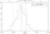 |
Fig. 4 Histogram of the secondary eclipse distribution in phase (lower axis) and in time (upper axis). All the secondary eclipses are sistematically below phase 0.5. The vertical dashed lines show the position of the four IAC80 IC-band secondary eclipses. |
5. Radial velocity and light curve fits
5.1. RV fitting procedure
We fit our RVs jointly with the primary and secondary measurements from Çakırlı et al. (2013) and Devor (2008). We fit a Keplerian orbit to the data using the rvfit code (Iglesias-Marzoa et al. 2015). This code is based on an adaptive simulated annealing (ASA) algorithm and can simultaneously fit the complete set of Keplerian parameters [ P,Tp,e,ω,γ,K1,K2 ] for the primary and secondary RV curves by χ2 function minimization. The uncertainties in the parameters can be computed from the Fisher matrix or using a Markov-Chain Monte Carlo method (MCMC). We chose this last method since it can deal with correlations between parameters. MCMC was run over 106 samples for each solution found with rvfit.
We ran a first fit to obtain initial parameter values and to check the significance of an elliptical orbit. In this first fit, we fixed only the orbital period to the value obtained in Sect. 4.6 and left all the other parameters free. This first solution was compatible with a low eccentric, e = 0.069 ± 0.016, orbit and a mass ratio of q = 0.558 ± 0.018. This elliptical orbit is confirmed by the small displacement in phase of the secondary eclipses shown in Sect. 4.6.
The dispersion in the RV measurements and the sinusoidal appearance of the RV data distribution can hide the subtle effect of a small eccentricity. To circumvent this limitation, we decided to constrain the eccentricity and the argument of the periastron using the Kepler light curves (see Sect. 5.2) and fix them to the values e = 0.0365 ± 0.0014 and ω = 92.8 ± 2.2 deg. This new fit yielded the values in Table 11. The fitted RV curve is shown in Fig. 5.
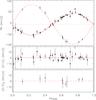 |
Fig. 5 RV curve fit and residuals. The continuous and dashed curves are the fits for the primary and secondary stars, respectively. The filled and empty circles are the RV measurements for the primary and secondary star respectively. The crosses are the RV measurements from Çakırlı et al. (2013). The dotted line in the upper panel is the value for γ. The phase was computed with Eq. (4). |
RV fitting results.
5.2. Light curves preliminary analysis with JKTEBOP
We used the detrended Kepler data to obtain an initial model of the light-curve without spots and to fix some initial parameters, namely ecosω and esinω. This allows us to start our combined analysis of the multiband light curves with initial values near the final solution once the spots are included in the analysis. For this goal we used JKTEBOP2 (Southworth et al. 2004), which is based on the EBOP code (Popper & Etzel 1981; Etzel 1981) and models the stars as triaxial ellipsoids. We fixed q, P and T0 from the ephemeris Eq. (4), and the solution of the RV curves (Sect. 5.1). We fit the following parameters: the sum and ratio of fractional radii, i.e. r1 + r2 and r1/r2, the orbital inclination i, the quantities esinω, ecosω, the surface bright of the secondary, and the light scale factor.
In this first stage, the effect of heating between the two components of the binary was not taken into account, since it was eliminated from the light curves when we detrended the out-of-eclipse variations. Therefore, the model coefficients associated with this effect were fixed to zero. In any case, we ran tests to confirm this effect was not noticeable. The third light contribution, l3, was fixed to the value calculated in Sect. 4.5. Tests fitting l3 yielded solutions with higher third light contributions, but poorer fits. We adopted a square-root limb darkening (LD) law (Diaz-Cordoves & Gimenez 1992; van Hamme 1993), with the LD coefficients interpolated from the tables provided by Claret & Bloemen (2011) and PHOENIX stellar models using the nominal Teff of 5560 ± 160 K and 3350 ± 50 K for the primary and secondary components. We adopted those values running preliminary PHOEBE tests with the optical IAC80 curves and the RV solution for a circular orbit. The PHOENIX models were selected based in their lower Teff limit, although the LD coefficient were computed only for Z = 0.0. The log g values were set to 4.5 and 5.0 for each component, respectively. For the gravity-brightening coefficients we used values from Claret & Bloemen (2011) for the same Teff.
To avoid problems caused by the long integration time of the Kepler data. we split up each observation into six points to undergo a numerical integration. The effect of this Kepler long integration time in light curves of eclipsing binaries (Coughlin et al. 2011) and exoplanet systems (Kipping 2010) is a known issue. These authors find that undersampling affects the morphological shape of the eclipses (transits), in such a way that they appear to be shallower and have a longer duration. This effect is most pronounced in eclipsing binaries with short periods and low sum of the fractional radii (r1 + r2) values. T-Cyg1-12664, with a r1 + r2 ≃ 0.1 is in the range where this effect can be noticed.
The heavy detrending applied to the Kepler light curve produces points deviating largely from the model in phases with strong light curve curvature near the center of the eclipses (see Fig. 7). Thus, a conservative sigma-clipping of 10σ was applied in the fitting process to discard these points. With this preliminary fit, we arrived at the solution shown in Figs. 6 and 7, where i = 86.87 ± 0.14, e = 0.0365 ± 0.0014, and ω = 92.8 ± 2.2. The resulting fractional radii are r1 = 0.07282 ± 0.00098 and r2 = 0.03300 ± 0.00050. The uncertainties in the fitted parameter were computed using a bootstrap analysis with 5000 synthetic datasets.
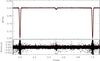 |
Fig. 6 JKTEBOP fit to the Kepler detrended light-curve. A detailed plot of the fits in the eclipses is shown in Fig. 7. |
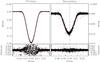 |
Fig. 7 Detail of the Fig. 6 showing the fit in the eclipses. Note the change in the vertical scale in the two plots and the small displacement of the secondary eclipse from phase 0.5, indicated with a vertical dashed line. |
5.3. Final light curve analysis with PHOEBE
To properly model the multiband light-curves of T-Cyg1-12664, we used PHysics Of Eclipsing BinariEs (PHOEBE, Prša & Zwitter 2005; Prša 2011). Given the low value of q for this system, the Roche lobe relative radii for each star (Eggleton 1983) are rRL1 ≃ 0.43 and rRL2 ≃ 0.33, well above the values obtained for the relative radii from the preliminary fit with JKTEBOP, so we selected a detached eclipsing binary model in PHOEBE.
We fit the IAC80 VRCIC light curves simultaneously with the Kepler light curve, but only using epochs of the Kepler light curve coeval with the ground-based observations. This is a necessary step to ensure that we are modeling the same spot configuration. Almost all IAC80 observations are coeval with Kepler’s Q6. We identified three epochs in which a primary and a contiguous secondary eclipses were observed simultaneously in all four bands. One epoch was discarded owing to unidentified systematics in the IAC80 data, which affect the level of the primary eclipse. The other two were selected for analysis with PHOEBE.
To avoid potential problems introduced by the ≃ 28 min low-cadence duty cycle of the Kepler light-curve, we performed a first fit using only the IAC80 light curves and the initial parameters derived from the detrended Kepler light curve in Sect. 5.2 to get a first set of parameters for the binary (radius, effective temperatures, etc). With these results, we ran a new fit, this time including the Kepler light curve to properly model the spots. This two-step approach helps the fitting of the system because 1) the IAC80 VRCIC light curves are best suited to constraining the effective temperatures, radii, and inclination of the system because of their high cadence during eclipses and finer spectral resolution and 2) the Kepler lightcurve have a better coverage of the out-of-eclipse phases, which allows us to model the spots. In the second fit, the physical and geometrical parameters of the binary are fixed and we only fit the spots. We iterate this two-step process until a satisfactory model is obtained and variations in the resultant parameters remain within the uncertainties for at least three consecutive fits. This approach has the disadvantage of being slower than the simultaneous fit of all the light curves but our preliminary test showed that the fitting results were notably better from the residuals point of view. The main advantage is that we retain both the physical information that are contained in the ground-based light curves and the excellent time coverage of the spot configuration contained in the Kepler light curves.
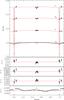 |
Fig. 8 Light curves of the T-Cyg1-12664 in the epoch Q6-1 and fitted model with the parameters of the first column in Table 12. From top to bottom (upper panel), filters IC, RC, V, and Kepler band. The ground-based observations are displaced vertically to shrink the plot. The lower panels show the residuals of these fits in the same order. |
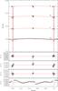 |
Fig. 9 Same figure as 8, but for the Q6-2 epoch. Note the jump in the Kepler photometry at phase 0.55 (see text). |
Given the large number of parameters in a complete binary system model, we tried to fix as many of them as possible beforehand, using all available information. We fixed the period and T0 to the values in the ephemeris equation in Sect. 4.6. The mass ratio q and γ were fixed from the RV solution in Table 11. The values for e and ω were fixed from the preliminary JKTEBOP analysis of the Kepler detrended light-curve in Sect. 2.1. The synchronicity parameter for the primary F1 was set to 1.041 ± 0.024, as obtained in Sect. 4.4. Although this is a very small value and it would not have practical effects on the shape of the star, we included it for completeness. For the secondary star, the synchronicity parameter F2 was assumed to be 1.0.
Teff1 was set to 5560 ± 160 K, as computed in Sect. 4.2, in agreement with the spectroscopic value and the colors derived from the absolute photometry. The albedos of the two components were set to A1 = A2 = 0.5 as given by Ruciński (1969), since the temperatures and spectral types are compatible with those of stars with convective envelopes. The values of the gravity-brightening exponents, β1 and β2, and those of the LD coefficients were interpolated from Claret & Bloemen (2011) for each passband. As in the case of the JKTEBOP preliminary light-curve analysis we used a square-root LD law (Diaz-Cordoves & Gimenez 1992). For the primary star these coefficient values were kept fixed since Teff1 does not change throughout the fitting process. For the secondary, we updated the coefficients values whenever necessary. As in Sect. 5.2, we used the same set of PHOENIX-based LD coefficients. This is because, during the fitting process, the Teff2 evolves below the 3500 K limit of the Kurucz LD tables. This occurred for all fitting attempts using the Phoebe(2010) or van Hamme (1993) LD coefficients, pointing to a Teff2 lower than 3500 K. This situation is most evident in the MCMC computations (see Sect. 5.5), some of them computing the merit function with Teff well below the 3500 K limit for the secondary.
The third light in the Kepler band was set to the value computed in Sect. 4.5. For the VRCIC band we set it to 0 since there is no evidence of a third body in the system and our photometry excludes the nearby red star. Even so, we run preliminary tests to check this assumption by fitting third light. The results were compatible with l3 = 0. For completeness, we also included mutual heating between the two components, but its effect is negligible in this system.
5.4. Spot modelling
A good spot model is critical for this system. Preliminary tests to decide on which component to place the spots showed that placing spots on the secondary had negligible effects on the light curve. This was expected, given the large difference in luminosity between the two components.
Our initial model consists of two spots on the primary located at phases φ ≃ −0.05 and φ ≃ 0.20 (λ ≃ 18° and λ ≃ 288°), and at a latitude of ~ 45°, since this is the latitude that some studies claim is more affected by spots (Hatzes 1995; Granzer et al. 2000). Our final spot solutions for the two epochs (see Figs. 8 and 9) show small deviations in the residuals with phase widths less than 0.5, so it cannot be produced by a single stellar spot. We tried to reduce these deviations by adding more spots to the primary without seeing significant improvements in the results. The Kepler light curve for the Q6-2 epoch shows a jump near phase φ ≃ −0.55, which prevents a better spot model fit, this jump is caused by small uncorrected drifts in the Kepler photometry, by the evolution in size or temperature of spots or by a combination of the two effects.
T-Cyg1-12664 parameters computed for two different epochs.
5.5. Final solutions
Taking into account the constraints and parameter values derived in the previous sections, the parameters fitted in the final model were the phase shift Δφ, the secondary temperature Teff2, the orbital inclination i, the two surface potentials Ω1, Ω2, the passband luminosities, and the spot parameters. The parameters common to the two columns were kept fixed during the fits and are the same for both epochs. For P and T0, the uncertainty is shown within parentheses. The final solutions for the two epochs analyzed are summarized in Table 12, while the fitted light curves and their residuals are shown in Figs. 8 and 9.
Aditionally, we used an MCMC wrapper for PHOEBE to re-fit the parameter values and to obtain a better estimation of the uncertainties in those parameters. The results of this computation are shown at the end of Table 12, while Figs. 11 and 12 show the parameter correlations from MCMC simulations and histograms of individual parameter distributions. To ensure the robustness of the fitted light curve model we ran a Gelman-Rubin diagnostics (Gelman & Rubin 1992) on the fitted parameters. Table 13 shows the  values, all of them very near 1.0, which indicate a robust solution.
Computed values from a Gelman-Rubin test for the fitted parameters in the two epochs analyzed.
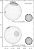 |
Fig. 10 Representation of the spot configurations of T-Cyg1-12664 in the (v,w) plane for the two epochs analyzed: the lower plot is for the Q6-1 epoch and the upper plot is for the Q6-2 epoch, which is displaced by an offset of 0.2 in the w axis. Both axes have units of relative radius. The stars are represented at orbital phase 0.020, just after the primary eclipse, and the secondary star is orbiting towards the right side. |
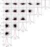 |
Fig. 11 Parameter correlations resulting from MCMC fit and histograms of individual parameter distributions for the Q6-1 epoch light curve. The red lines show the values adopted in this work from the maximum of the histograms. Dashed vertical lines indicated the 68.3% confidence interval. |
The fractional radii of each star are similar between the two epochs, but with differences slightly larger than the computed uncertainties. The departure from a perfectly spherical shape is very small (≃0.07% for the primary and ≃0.013% for the secondary), as expected from the wide separation between the stars and their small masses. The position of the spots differs significantly between epochs, being the most stable parameter the longitude, which is tightly constrained by the light curve dips. The differences between models for Teff and the radii could be related to this variation in the spots configuration, as noted by Morales et al. (2010). In Fig. 10, we show a representation of the spot configuration resulting from our analysis in the two epochs analyzed.
6. The system of T-Cyg1-12664
6.1. Absolute parameters
From the results in Tables 11 and 12, we computed the absolute parameters for the components of T-Cyg1-12664. Those results are summarized in Table 14. The adopted radii, Teff2 and orbital inclination were computed from the mean for the two fits and their uncertainties are the standard deviations. The secondary is an M3V star, based on its effective temperature (Mamajek 2015). For the solar values we used the recommended IAU values Teff ⊙ = 5772 K, log g⊙ = 4.438, Mbol ⊙ = 4.74 (IAU Inter-Division A-G Working Group on Nominal Units for Stellar & Planetary Astronomy 2015; Prša et al. 2016). The bolometric corrections were computed using the BC scale by Flower (1996) (but see Torres 2010, Sect. 2).
Absolute dimensions and main physical parameters of the T-Cyg1-12664 system components.
The uncertainties in the masses are 6.7% for M1 and 4.5% for M2, which are consistent with the uncertainties in the RV amplitudes. The uncertainties in the radii are 2.1% for R1 and 2.3% for R2. The radii are in good agreement with those obtained from the JKTEBOP model without spots (see Sect. 5.2), which resulted in R1 = 0.803 ± 0.019 R⊙ and R2 = 0.364 ± 0.0089 R⊙. The difference in the secondary radius can be attributed to the strong impact of the spots in the light curve, compared with the depth of the secondary eclipse. The orbit is nearly edge-on with an inclination of i = 86.969 ± 0.056 degrees, adopted from the mean of the two fits. The luminosity ratio in the visual band is LB/LA = 0.0034 ± 0.0026 and its uncertainty reflects the uncertainty of the secondary absolute magnitude. Given the uncertainties in the Teff scale, we adopted uncertainties of ±1 in the spectral types.
Hut (1981) showed that, in a eccentric orbit, the rotational angular velocity of a star will tend to synchronize with the velocity at periastron as a consecuence of the strong dependence of the tidal forces on distance, a condition called pseudosynchronization. With the value of the orbital eccentricity, we computed the synchronicity parameter for the case of pseudosynchronization (Hut 1981, Eq. (44)) to be Frmpseudo = 1.0765 ± 0.0031, which is slighty larger than our measured syncronicity parameter F = 1.041 ± 0.024. The difference could be due to differential rotation with spot latitude, in which case the spot’s rotation would not be representative of the actual stellar rotation. In addition, the result from the Lomb-Scargle periodograms could be biased by the fact that there are, at least two groups of spots, making the resulting rotation period a mean of the movement of the two groups. Given the small eccentricity measured, we can consider that the orbit is circularized, and this will impose a lower limit for the age of the system because of the long time required to achieve this state. Using tidal friction theory Zahn (1977), we find the time scale for synchronization is tsync ≃ 6 Myr, and the time scale for circularization tcirc ≃ 2 Gyr, which sets a minimum age for the system.
6.2. Distance, space velocities and age
Combining the absolute V magnitudes of the two components, we obtain an absolute V magnitude for T-Cyg1-12664 of MVtot = 5.52 ± 0.14. Given the apparent visual magnitude of the system V = 13.299 ± 0.005 (see Sect. 4.1), this gives an unreddened distance modulus of m−M = 7.78, which translates into a distance of d = 360 ± 22 pc.
We computed the (U,V,W)3 space velocities of the system using the Johnson & Soderblom (1987) algorithm, the distance computed above, the system’s systemic velocity (see Sect. 5.1) and the 2MASS proper motion measurements (Cutri 2003): μαcosδ = −18 ± 6 mas yr-1, μδ = −6 ± 2 mas yr-1. The resultant velocities are U = 17.5 ± 3.3 km s-1, V = −11.1 ± 1.7 km s-1, W = 11.5 ± 5.9 km s-1, and a total space velocity of S = 23.7 ± 7.0 km s-1. These velocities place the binary near the border of the area defined by Eggen (1989) as belonging to the young galactic disk. The velocities do not exactly agree with the criteria of Leggett (1992) (−50 < U < 20, −30 < V < 0, −25 < W < 10, all in km s-1) but they lie very near the limit. Also the binary is not within any known early-type or late-type population tracer (Skuljan et al. 1999), although it lies near the V-middle branch for late-type stars (U = 17.8, V = −15.37) km s-1. In addition, it cannot be related to any known moving group (Montes et al. 2001; Maldonado et al. 2010). Therefore, we cannot impose constraints on the age of the system based on kinematic criteria. However, based on circularization and synchronization times for a P≃ 4.13 days orbit, we can speculate on an age of at least 2 Gyr for the system. This age rules out the possibility of T-Cyg1-12664 being pre-main-sequence, and is a clue that its components are main-sequence stars.
In Fig. 13, we plotted the Baraffe et al. (1998) (hereafter BCAH98) isocrones for [M/H] = 0.0 (in black) and for [M/H] = −0.5 (in red). All the isochrones older than log(age) = 8.0 fit equally well the components of this system. The primary is better fitted by isochrones for [M/H] = −0.5, and the secondary is better fitted by isochrones for [M/H] = 0.0. The effect of the subsolar metallicity could explain the primary’s effective temperature, but not its oversize. However, the difference in the space parameter for the two sets of isochrones for the two metallicities is smaller than the uncertainties in the computed stellar parameters, and the uncertainty about the actual metallicity of the system remains. A specific metallicity analysis for this system would resolve this question. All that can be said is that this system is old and we can safely discard a young pre-main-sequence system.
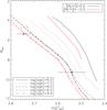 |
Fig. 13 Position in the Mbol-log Teff diagram of the two components in the system of T-Cyg1-12664. BCAH98 isochrones are for [M/H] = 0.0 (black) and [M/H] = −0.5 (red) for log (age) = 6.0, 7.0, 8.0, 9.0 and 9.9. |
6.3. Comparison with models and previous analyses
Low-mass stars in eclipsing binaries are commonly found to have larger radii and lower effective temperatures than those predicted by current models. In Figs. 14 and 15, we compare the mass, radius, and temperature of the components of T-Cyg1-12664 to models and to other binaries. The models in the figures are those of Baraffe et al. (1998), Dotter et al. (2008), Girardi et al. (2000), and Yi et al. (2001), all of them for solar metallicity (Z = 0.02) and an age of 3 Gyr, which cover the entire low-mas regime. We adopt those values since they provide a good fit to the overall sample of mass-radius measurements of main sequence low-mass stars in the literature, and also the secondary of T-Cyg-12664, although not the primary. We note, however, that this model is used for illustration of the entire observational sample of low-mass stars, and is not a fit to the T-Cyg-12664.
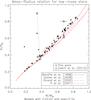 |
Fig. 14 Mass-radius relations of stars between 0.2 and 1.0 M⊙ predicted by four stellar models (see text). The filled circles represent well-known LMDEB, used as benchmarks for the models. The triangles represent the location of T-Cyg1-12664 in the Çakırlı et al. (2013) paper and the diamonds are our solution for this system. We connect the two solutions for the primary and the secondary with a dotted line to guide the eye to the difference in the physical parameters that arise from the two solutions. Metallicity and age are set for reference of the whole set of stars and they are not a fit to the T-Cyg1-12664 parameters. |
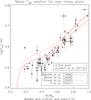 |
Fig. 15 Mass-log Teff relations for the same LMDEB systems as in Fig. 14. Again, we connected with a dotted line the solutions derived by Çakırlı et al. (2013) for the primary and secondary with our solutions. Metallicity and age are set for reference of the whole set of stars and they are not a fit to the T-Cyg1-12664 parameters. |
The mixing length parameter for the Baraffe et al. (1998) model is α = l/Hp = 1. The other binaries included in the figure (listed in Table 15) are all the current systems with masses and radii measured with relative precisions better than 7%. We also included the previous measurements by Çakırlı et al. (2013) for this system in the figures.
Our results show agreement between the parameters of the secondary and models, in particular with the predictions from Baraffe et al. (1998) and Dotter et al. (2008). This is a particularly important result, since the secondary has a mass very close to the fully convective stellar boundary at ~0.35 M⊙. The parameters of the primary, on the other hand, deviate significantly from the model predictions, both in the mass-radius and the mass-log Teff plots. The primary is oversized ~34% over the value of the radius predicted by the models. This deviation is larger than any other well measured binary components in this mass range. In the mass-log Teff plane, the primary exhibits a very high effective temperature, being over 1000 K hotter than what models for a star of that mass predict. We must emphasize that the temperature has been measured directly from the photometric colors, which are found to be consistent among photometric systems, and spectroscopy (see Sects. 4.2 and 4.3), and is not a result of the modeling process. At present, we can not find an explanation for this discrepancy, but there is at least one other low-mass binary that exhibits this effect (see Gómez Maqueo Chew et al. 2014).
List of benchmark low-mass components in eclipsing binaries taken from the literature.
Our results also differ from those of Çakırlı et al. (2013), the main differences in the analysis being the setting of a reliable set of color indexes, the treatment of the eccentricity, and the processing of the Kepler light curves. These differences can explain the disagreement in the parameters obtain from the light curves, i.e. the radii, the Teff, and luminosity-related quantities. Only the masses, derived from the RV curves, are similar, although our secondary mass is slightly larger. We attribute this to improvements in the RV curve of the primary and the detection of a slight eccentricity for the system.
T-Cyg1-12664 was also analyzed by Prša et al. (2011) using Eclipsing Binaries via Artificial Intelligence (EBAI, Prša et al. 2008) on a survey of eclipsing binaries found in the Kepler field of view. EBAI relies on trained neural networks to yield principal parameters for all the binary stars in the catalog. In the accompanying table, we found the following values: Teff = 5669 K, log g = 4.308, sini = 0.99441, esinω = 0.04452, ecosω = −0.35923, T2/T1 = 0.5965, and ρ1 + ρ2 = 0.10881, with an effective temperature in reasonable agreement with the value obtained from our photometry. The same authors published the Kepler Eclipsing Binary Catalog4 (KEB) online. A query of this catalog using the Kepler name of the system (KIC 10935310) returns a different set of physical parameters: sini = 0.99479, esinω = 0.05606, ecosω = 0.22161, T2/T1 = 0.78209, and ρ1 + ρ2 = 0.13246. The values for e and ω arising from both solutions are incompatible with our radial velocity and photometric curves. However, a new analysis of the Kepler dataset by the Kepler EB team gives ω = 94.2 degrees and e = 0.0372, which are consistent with our values (Prša, priv. comm.).
7. Conclusions
Our analysis of the T-Cyg1-12664 low-mass eclipsing binary system shows a different picture from other published analyses (Devor 2008; Çakırlı et al. 2013). The main differences between our analysis and the previous ones are: the measurement of consistent and accurate calibrated magnitudes in the optical bands, which lead to a precise determination of the Teff scale; a careful treatment of the contamination by nearby stars in the Kepler band photometry, with a direct impact in the orbital inclination and, thus, in the fractional radii; and the discovery of a small displacement of the secondary eclipse which lead to the analysis of the system as an eccentric binary.
Our resuls for this system show an oversized primary with M1 = 0.680 ± 0.045 M⊙, R1 = 0.799 ± 0.017 R⊙, and Teff1 = 5560 ± 160 K, in a slightly eccentric orbit with e = 0.0365 ± 0.0014 and i = 86.969 ± 0.056. The secondary is a star near the fully convective stellar mass boundary with M2 = 0.376 ± 0.017 M⊙, R2 = 0.3475 ± 0.0081 R⊙, and Teff2 = 3460 ± 210 K. Its parameters agree well with models.
The faintness of the secondary component is a drawback in the measurement of radial velocities for this system, which only shows the radial velocities of the primary with telescopes of medium size. This prevents us from directly measuring q for this system and forces us to rely on published radial velocities for the secondary. The secondary star appears to have a mass in a key region for models, i.e. the transition to fully convective stars, which remains poorly sampled by observations. Therefore, new measurements of the secondary radial velocity curve of this system using, for example, near-IR spectroscopy will be important.
Avaliable at http://keplergo.arc.nasa.gov/CalibrationResponse.shtml
JKTEBOP is written in FORTRAN 77 and the source code is available at http://www.astro.keele.ac.uk/jktcodes/jktebop.html
Positive values of U, V, and W indicate velocities toward the Galactic center, Galactic rotation, and north Galactic pole, respectively.
Avaliable at http://keplerebs.villanova.edu/v2
Acknowledgments
We thank the referee A. Prša for helpful comments on the manuscript. This article is based on observations made with the IAC80 telescope operated on the island of Tenerife by the Instituto de Astrofisica de Canarias in the Spanish Observatorio del Teide, on observations obtained with the Apache Point Observatory 3.5-m telescope, which is owned and operated by the Astrophysical Research Consortium. and on observations at Kitt Peak National Observatory, National Optical Astronomy Observatory (NOAO Prop. IDs: 2011A-0392; PI: J. Coughlin), which is operated by the Association of Universities for Research in Astronomy (AURA) under cooperative agreement with the National Science Foundation. IRAF is distributed by the National Optical Astronomy Observatory, which is operated by the Association of Universities for Research in Astronomy (AURA) under a cooperative agreement with the National Science Foundation. This research has made use of the SIMBAD database, operated at CDS, Strasbourg, France, and of NASA’s Astrophysics Data System Bibliographic Services. Also, it used data products from the Two Micron All Sky Survey. Some of the data presented in this paper were obtained from the Mikulski Archive for Space Telescopes (MAST). This paper includes data collected by the Kepler mission. Funding for the Kepler mission is provided by the NASA Science Mission directorate. R.I.M. acknowledges support through the Programa de Acceso a Instalaciones Cientificas Singulares (E/309290). J.L.C. acknowledges support through a National Science Foundation Graduate Research Fellowship.
References
- Alonso, R., Brown, T. M., Torres, G., et al. 2004, ApJ, 613, L153 [NASA ADS] [CrossRef] [Google Scholar]
- Arribas, S., & Martinez Roger, C. 1988, A&A, 206, 63 [NASA ADS] [Google Scholar]
- Ballesteros, F. J. 2012, EPL, 97, 34008 [NASA ADS] [CrossRef] [EDP Sciences] [Google Scholar]
- Baraffe, I., Chabrier, G., Allard, F., & Hauschildt, P. H. 1998, A&A, 337, 403 [NASA ADS] [Google Scholar]
- Bayless, A. J., & Orosz, J. A. 2006, ApJ, 651, 1155 [NASA ADS] [CrossRef] [Google Scholar]
- Behr, B. B. 2003, ApJS, 149, 67 [NASA ADS] [CrossRef] [Google Scholar]
- Bessell, M. S. 1979, PASP, 91, 589 [NASA ADS] [CrossRef] [Google Scholar]
- Bessell, M. S. 1991, AJ, 101, 662 [NASA ADS] [CrossRef] [Google Scholar]
- Birkby, J., Nefs, B., Hodgkin, S., et al. 2012, MNRAS, 426, 1507 [NASA ADS] [CrossRef] [Google Scholar]
- Brogna, P. 2006, Ph.D. Thesis, San Francisco State University, USA [Google Scholar]
- Brown, T. M., Latham, D. W., Everett, M. E., & Esquerdo, G. A. 2011, AJ, 142, 112 [NASA ADS] [CrossRef] [Google Scholar]
- Çakırlı, Ö. 2013, New A, 22, 15 [NASA ADS] [CrossRef] [Google Scholar]
- Çakırlı, Ö., İbanoǧlu, C., & Sipahi, E. 2013, MNRAS, 429, 85 [NASA ADS] [CrossRef] [Google Scholar]
- Carter, J. A., Fabrycky, D. C., Ragozzine, D., et al. 2011, Science, 331, 562 [NASA ADS] [CrossRef] [PubMed] [Google Scholar]
- Claret, A., & Bloemen, S. 2011, A&A, 529, A75 [NASA ADS] [CrossRef] [EDP Sciences] [Google Scholar]
- Clausen, J. V., Bruntt, H., Claret, A., et al. 2009, A&A, 502, 253 [NASA ADS] [CrossRef] [EDP Sciences] [Google Scholar]
- Coughlin, J. L. 2012, Ph.D. Thesis, New Mexico State University, USA [Google Scholar]
- Coughlin, J. L., López-Morales, M., Harrison, T. E., Ule, N., & Hoffman, D. I. 2011, AJ, 141, 78 [NASA ADS] [CrossRef] [Google Scholar]
- Cox, A. N. 2000, Allen’s Astrophysical Quantities, 4th edn. (New York: AIP) [Google Scholar]
- Cutri, R.M., et al. 2003, The IRSA 2MASS All-Sky Point Source Catalogue, Tech. Rep., NASA/IPAC Infrared Science Archive, available at http://irsa.ipac.caltech.edu/applications/Gator/ [Google Scholar]
- Devor, J. 2008, Ph.D. Thesis, Harvard University, USA [Google Scholar]
- Devor, J., Charbonneau, D., O’Donovan, F. T., Mandushev, G., & Torres, G. 2008a, AJ, 135, 850 [NASA ADS] [CrossRef] [Google Scholar]
- Devor, J., Charbonneau, D., Torres, G., et al. 2008b, ApJ, 687, 1253 [NASA ADS] [CrossRef] [Google Scholar]
- Diaz-Cordoves, J., & Gimenez, A. 1992, A&A, 259, 227 [NASA ADS] [Google Scholar]
- Dotter, A., Chaboyer, B., Jevremović, D., et al. 2008, ApJS, 178, 89 [NASA ADS] [CrossRef] [Google Scholar]
- Eastman, J., Siverd, R., & Gaudi, B. S. 2010, PASP, 122, 935 [NASA ADS] [CrossRef] [Google Scholar]
- Eggen, O. J. 1989, PASP, 101, 366 [NASA ADS] [CrossRef] [Google Scholar]
- Eggleton, P. P. 1983, ApJ, 268, 368 [NASA ADS] [CrossRef] [Google Scholar]
- Eisenstein, D. J., Weinberg, D. H., Agol, E., et al. 2011, AJ, 142, 72 [Google Scholar]
- Etzel, P. B. 1981, in Photometric and Spectroscopic Binary Systems, eds. E. B. Carling, & Z. Kopal, 111 [Google Scholar]
- Everett, M. E., Howell, S. B., & Kinemuchi, K. 2012, PASP, 124, 316 [NASA ADS] [CrossRef] [Google Scholar]
- Flower, P. J. 1996, ApJ, 469, 355 [NASA ADS] [CrossRef] [Google Scholar]
- Fukugita, M., Yasuda, N., Doi, M., Gunn, J. E., & York, D. G. 2011, AJ, 141, 47 [NASA ADS] [CrossRef] [Google Scholar]
- Gelman, A., & Rubin, D. 1992, Stat. Science, 7, 457 [Google Scholar]
- Girardi, L., Bressan, A., Bertelli, G., & Chiosi, C. 2000, A&AS, 141, 371 [NASA ADS] [CrossRef] [EDP Sciences] [Google Scholar]
- Gómez Maqueo Chew, Y., Morales, J. C., Faedi, F., et al. 2014, A&A, 572, A50 [NASA ADS] [CrossRef] [EDP Sciences] [Google Scholar]
- Granzer, T., Schüssler, M., Caligari, P., & Strassmeier, K. G. 2000, A&A, 355, 1087 [NASA ADS] [Google Scholar]
- Hatzes, A. P. 1995, in IAU Symp., 176, 90 [Google Scholar]
- Hełminiak, K. G., & Konacki, M. 2011, A&A, 526, A29 [NASA ADS] [CrossRef] [EDP Sciences] [Google Scholar]
- Hełminiak, K. G., Konacki, M., Złoczewski, K., et al. 2011, A&A, 527, A14 [NASA ADS] [CrossRef] [EDP Sciences] [Google Scholar]
- Hełminiak, K. G., Konacki, M., RóŻyczka, M., et al. 2012, MNRAS, 425, 1245 [NASA ADS] [CrossRef] [Google Scholar]
- Hełminiak, K. G., Brahm, R., Ratajczak, M., et al. 2014, A&A, 567, A64 [NASA ADS] [CrossRef] [EDP Sciences] [Google Scholar]
- Houdashelt, M. L., Bell, R. A., & Sweigart, A. V. 2000, AJ, 119, 1448 [Google Scholar]
- Hut, P. 1981, A&A, 99, 126 [NASA ADS] [Google Scholar]
- IAU Inter-Division A-G Working Group on Nominal Units for Stellar & Planetary Astronomy 2015, Resolution B2 on recommended zero points for the absolute and apparent bolometric magnitude scales, Tech. Rep., IAU [Google Scholar]
- Iglesias-Marzoa, R., López-Morales, M., & Jesús Arévalo Morales, M. 2015, PASP, 127, 567 [NASA ADS] [CrossRef] [Google Scholar]
- Irwin, J., Charbonneau, D., Berta, Z. K., et al. 2009, ApJ, 701, 1436 [NASA ADS] [CrossRef] [Google Scholar]
- Irwin, J. M., Quinn, S. N., Berta, Z. K., et al. 2011, ApJ, 742, 123 [NASA ADS] [CrossRef] [Google Scholar]
- Ivezić, Ž., Sesar, B., Jurić, M., et al. 2008, ApJ, 684, 287 [NASA ADS] [CrossRef] [Google Scholar]
- Jenkins, J. M., Caldwell, D. A., Chandrasekaran, H., et al. 2010, ApJ, 713, L87 [NASA ADS] [CrossRef] [Google Scholar]
- Johnson, D. R. H., & Soderblom, D. R. 1987, AJ, 93, 864 [NASA ADS] [CrossRef] [Google Scholar]
- Kipping, D. M. 2010, MNRAS, 408, 1758 [NASA ADS] [CrossRef] [Google Scholar]
- Kraus, A. L., Tucker, R. A., Thompson, M. I., Craine, E. R., & Hillenbrand, L. A. 2011, ApJ, 728, 48 [NASA ADS] [CrossRef] [Google Scholar]
- Kurucz, R. L. 1993, The 1993 Kurucz Stellar Atmospheres Atlas, available at ftp://ftp.stsci.edu/cdbs/grid/kurucz93models [Google Scholar]
- Landolt, A. U. 2009, AJ, 137, 4186 [NASA ADS] [CrossRef] [Google Scholar]
- Lanza, A. F., Das Chagas, M. L., & De Medeiros, J. R. 2014, A&A, 564, A50 [NASA ADS] [CrossRef] [EDP Sciences] [Google Scholar]
- Leggett, S. K. 1992, ApJS, 82, 351 [NASA ADS] [CrossRef] [Google Scholar]
- Lejeune, T., Cuisinier, F., & Buser, R. 1998, A&AS, 130, 65 [NASA ADS] [CrossRef] [EDP Sciences] [Google Scholar]
- López-Morales, M., & Bonanos, A. Z. 2008, ApJ, 685, L47 [NASA ADS] [CrossRef] [Google Scholar]
- López-Morales, M., & Ribas, I. 2005, ApJ, 631, 1120 [NASA ADS] [CrossRef] [Google Scholar]
- Maldonado, J., Martínez-Arnáiz, R. M., Eiroa, C., Montes, D., & Montesinos, B. 2010, A&A, 521, A12 [NASA ADS] [CrossRef] [EDP Sciences] [Google Scholar]
- Mamajek, E. E. 2015, A Modern Mean Stellar Color and Effective Temperature Sequence for O9V-Y0V Dwarf Stars, available at http://www.pas.rochester.edu/~emamajek/EEM_dwarf_UBVIJHK_colors_Teff.txt [Google Scholar]
- Masana, E., Jordi, C., & Ribas, I. 2006, A&A, 450, 735 [NASA ADS] [CrossRef] [EDP Sciences] [Google Scholar]
- Merline, W. J., & Howell, S. B. 1995, Exp. Astron., 6, 163 [NASA ADS] [CrossRef] [Google Scholar]
- Montes, D., López-Santiago, J., Gálvez, M. C., et al. 2001, MNRAS, 328, 45 [NASA ADS] [CrossRef] [MathSciNet] [Google Scholar]
- Morales, J. C., Ribas, I., Jordi, C., et al. 2009a, ApJ, 691, 1400 [NASA ADS] [CrossRef] [Google Scholar]
- Morales, J. C., Torres, G., Marschall, L. A., & Brehm, W. 2009b, ApJ, 707, 671 [NASA ADS] [CrossRef] [Google Scholar]
- Morales, J. C., Gallardo, J., Ribas, I., et al. 2010, ApJ, 718, 502 [NASA ADS] [CrossRef] [Google Scholar]
- Moro, D., & Munari, U. 2000, A&AS, 147, 361 [NASA ADS] [CrossRef] [EDP Sciences] [Google Scholar]
- Munari, U., Sordo, R., Castelli, F., & Zwitter, T. 2005, A&A, 442, 1127 [NASA ADS] [CrossRef] [EDP Sciences] [Google Scholar]
- Östensen, R. 2000, Ph.D. Thesis, University of Trömso, Norway [Google Scholar]
- Östensen, R., & Solheim, J.-E. 2000, Baltic Astron., 9, 411 [Google Scholar]
- Popper, D. M., & Etzel, P. B. 1981, AJ, 86, 102 [NASA ADS] [CrossRef] [Google Scholar]
- Prša, A. 2011, PHOEBE Scientific Reference (Philadelphia: SIAM) [Google Scholar]
- Prša, A., & Zwitter, T. 2005, ApJ, 628, 426 [NASA ADS] [CrossRef] [Google Scholar]
- Prša, A., Guinan, E. F., Devinney, E. J., et al. 2008, ApJ, 687, 542 [NASA ADS] [CrossRef] [Google Scholar]
- Prša, A., Batalha, N., Slawson, R. W., et al. 2011, AJ, 141, 83 [NASA ADS] [CrossRef] [Google Scholar]
- Prša, A., Harmanec, P., Torres, G., et al. 2016, AJ, 152, 41 [NASA ADS] [CrossRef] [Google Scholar]
- Reinhold, T., & Arlt, R. 2015, A&A, 576, A15 [NASA ADS] [CrossRef] [EDP Sciences] [Google Scholar]
- Ribas, I. 2003, A&A, 398, 239 [NASA ADS] [CrossRef] [EDP Sciences] [Google Scholar]
- Rozyczka, M., Kaluzny, J., Pietrukowicz, P., et al. 2009, Acta Astron., 59, 385 [Google Scholar]
- Ruciński, S. M. 1969, Acta Astron., 19, 245 [Google Scholar]
- Scargle, J. D. 1982, ApJ, 263, 835 [NASA ADS] [CrossRef] [Google Scholar]
- Skrutskie, M. F., Cutri, R. M., Stiening, R., et al. 2006, AJ, 131, 1163 [NASA ADS] [CrossRef] [Google Scholar]
- Skuljan, J., Hearnshaw, J. B., & Cottrell, P. L. 1999, MNRAS, 308, 731 [NASA ADS] [CrossRef] [Google Scholar]
- Slawson, R. W., Prša, A., Welsh, W. F., et al. 2011, AJ, 142, 160 [NASA ADS] [CrossRef] [Google Scholar]
- Southworth, J., Maxted, P. F. L., & Smalley, B. 2004, MNRAS, 351, 1277 [NASA ADS] [CrossRef] [Google Scholar]
- Torres, G. 2010, AJ, 140, 1158 [NASA ADS] [CrossRef] [Google Scholar]
- Torres, G., & Ribas, I. 2002, ApJ, 567, 1140 [NASA ADS] [CrossRef] [Google Scholar]
- Vaccaro, T. R., Rudkin, M., Kawka, A., et al. 2007, ApJ, 661, 1112 [NASA ADS] [CrossRef] [Google Scholar]
- van Dokkum, P. G. 2001, PASP, 113, 1420 [NASA ADS] [CrossRef] [Google Scholar]
- van Hamme, W. 1993, AJ, 106, 2096 [NASA ADS] [CrossRef] [Google Scholar]
- Yi, S., Demarque, P., Kim, Y.-C., et al. 2001, ApJS, 136, 417 [NASA ADS] [CrossRef] [Google Scholar]
- Zahn, J.-P. 1977, A&A, 57, 383 [NASA ADS] [Google Scholar]
- Zucker, S., & Mazeh, T. 1994, ApJ, 420, 806 [NASA ADS] [CrossRef] [EDP Sciences] [MathSciNet] [Google Scholar]
All Tables
Photometry in several bands for T-Cyg1-12664 obtained from photometric catalogs.
Observed Landolt fields. The number of measurements is the global count for different air masses.
Calibrated magnitudes and color indices for T-Cyg1 obtained from our photometric calibration.
Mean effective temperature estimations resulting from our photometric calibration, 2MASS and SDSS photometry and our spectroscopy for T-Cyg1-12664.
Computed values from a Gelman-Rubin test for the fitted parameters in the two epochs analyzed.
Absolute dimensions and main physical parameters of the T-Cyg1-12664 system components.
List of benchmark low-mass components in eclipsing binaries taken from the literature.
All Figures
|
Fig. 1 Fit of an order 300 Legendre polynomial to the Kepler data in quarter 6. The upper panel shows the out-of-eclipse light curve and the fit (red line). The lower panel shows the residuals of the fit. |
| In the text | |
|
Fig. 2 Effect of the detrending over the phased light curve of Q6 quarter. Upper panel shows the raw light curve and lower panel shows the light curve after applying the Legendre polynomial fitted in Fig. 1. |
| In the text | |
|
Fig. 3 Comparison between the absolute optical and 2MASS photometry with the synthetic photometry obtained for a Kurucz model with Teff = 5500 K, log g = 4.5, and [ M / H ] = −0.5. The uncertainties in the upper panel are smaller than the point sizes. |
| In the text | |
|
Fig. 4 Histogram of the secondary eclipse distribution in phase (lower axis) and in time (upper axis). All the secondary eclipses are sistematically below phase 0.5. The vertical dashed lines show the position of the four IAC80 IC-band secondary eclipses. |
| In the text | |
|
Fig. 5 RV curve fit and residuals. The continuous and dashed curves are the fits for the primary and secondary stars, respectively. The filled and empty circles are the RV measurements for the primary and secondary star respectively. The crosses are the RV measurements from Çakırlı et al. (2013). The dotted line in the upper panel is the value for γ. The phase was computed with Eq. (4). |
| In the text | |
|
Fig. 6 JKTEBOP fit to the Kepler detrended light-curve. A detailed plot of the fits in the eclipses is shown in Fig. 7. |
| In the text | |
|
Fig. 7 Detail of the Fig. 6 showing the fit in the eclipses. Note the change in the vertical scale in the two plots and the small displacement of the secondary eclipse from phase 0.5, indicated with a vertical dashed line. |
| In the text | |
|
Fig. 8 Light curves of the T-Cyg1-12664 in the epoch Q6-1 and fitted model with the parameters of the first column in Table 12. From top to bottom (upper panel), filters IC, RC, V, and Kepler band. The ground-based observations are displaced vertically to shrink the plot. The lower panels show the residuals of these fits in the same order. |
| In the text | |
|
Fig. 9 Same figure as 8, but for the Q6-2 epoch. Note the jump in the Kepler photometry at phase 0.55 (see text). |
| In the text | |
|
Fig. 10 Representation of the spot configurations of T-Cyg1-12664 in the (v,w) plane for the two epochs analyzed: the lower plot is for the Q6-1 epoch and the upper plot is for the Q6-2 epoch, which is displaced by an offset of 0.2 in the w axis. Both axes have units of relative radius. The stars are represented at orbital phase 0.020, just after the primary eclipse, and the secondary star is orbiting towards the right side. |
| In the text | |
|
Fig. 11 Parameter correlations resulting from MCMC fit and histograms of individual parameter distributions for the Q6-1 epoch light curve. The red lines show the values adopted in this work from the maximum of the histograms. Dashed vertical lines indicated the 68.3% confidence interval. |
| In the text | |
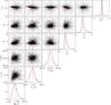 |
Fig. 12 Same as Fig. 11 but for the Q6-2 epoch light curve. |
| In the text | |
|
Fig. 13 Position in the Mbol-log Teff diagram of the two components in the system of T-Cyg1-12664. BCAH98 isochrones are for [M/H] = 0.0 (black) and [M/H] = −0.5 (red) for log (age) = 6.0, 7.0, 8.0, 9.0 and 9.9. |
| In the text | |
|
Fig. 14 Mass-radius relations of stars between 0.2 and 1.0 M⊙ predicted by four stellar models (see text). The filled circles represent well-known LMDEB, used as benchmarks for the models. The triangles represent the location of T-Cyg1-12664 in the Çakırlı et al. (2013) paper and the diamonds are our solution for this system. We connect the two solutions for the primary and the secondary with a dotted line to guide the eye to the difference in the physical parameters that arise from the two solutions. Metallicity and age are set for reference of the whole set of stars and they are not a fit to the T-Cyg1-12664 parameters. |
| In the text | |
|
Fig. 15 Mass-log Teff relations for the same LMDEB systems as in Fig. 14. Again, we connected with a dotted line the solutions derived by Çakırlı et al. (2013) for the primary and secondary with our solutions. Metallicity and age are set for reference of the whole set of stars and they are not a fit to the T-Cyg1-12664 parameters. |
| In the text | |
Current usage metrics show cumulative count of Article Views (full-text article views including HTML views, PDF and ePub downloads, according to the available data) and Abstracts Views on Vision4Press platform.
Data correspond to usage on the plateform after 2015. The current usage metrics is available 48-96 hours after online publication and is updated daily on week days.
Initial download of the metrics may take a while.