| Issue |
A&A
Volume 599, March 2017
|
|
|---|---|---|
| Article Number | A58 | |
| Number of page(s) | 12 | |
| Section | The Sun | |
| DOI | https://doi.org/10.1051/0004-6361/201629758 | |
| Published online | 01 March 2017 | |
Connection between solar activity cycles and grand minima generation
1 LESIA – Observatoire de Paris, 5 place Jules Janssen, 92190 Meudon, France
e-mail: This email address is being protected from spambots. You need JavaScript enabled to view it.
2 Dipartimento di Fisica, Università della Calabria, Ponte P. Bucci Cubo 31C, 87036 Rende (CS), Italy
3 INAF–IAPS, via Fosso del Cavaliere 100, 00133 Roma, Italy
Received: 20 September 2016
Accepted: 28 November 2016
Abstract
Aims. The revised dataset of sunspot and group numbers (released by WDC-SILSO) and the sunspot number reconstruction based on dendrochronologically dated radiocarbon concentrations have been analyzed to provide a deeper characterization of the solar activity main periodicities and to investigate the role of the Gleissberg and Suess cycles in the grand minima occurrence.
Methods. Empirical mode decomposition (EMD) has been used to isolate the time behavior of the different solar activity periodicities. A general consistency among the results from all the analyzed datasets verifies the reliability of the EMD approach.
Results. The analysis on the revised sunspot data indicates that the highest energy content is associated with the Schwabe cycle. In correspondence with the grand minima (Maunder and Dalton), the frequency of this cycle changes to longer timescales of ~14 yr. The Gleissberg and Suess cycles, with timescales of 60−120 yr and ~ 200−300 yr, respectively, represent the most energetic contribution to sunspot number reconstruction records and are both found to be characterized by multiple scales of oscillation. The grand minima generation and the origin of the two expected distinct types of grand minima, Maunder and longer Spörer-like, are naturally explained through the EMD approach. We found that the grand minima sequence is produced by the coupling between Gleissberg and Suess cycles, the latter being responsible for the most intense and longest Spörer-like minima (with typical duration longer than 80 yr). Finally, we identified a non-solar component, characterized by a very long scale oscillation of ~ 7000 yr, and the Hallstatt cycle (~ 2000 yr), likely due to the solar activity.
Conclusions. These results provide new observational constraints on the properties of the solar cycle periodicities, the grand minima generation, and thus the long-term behavior of the solar dynamo.
Key words: Sun: activity / sunspots / methods: data analysis
© ESO, 2017
1. Introduction
One of the most fascinating phenomena in astrophysics is the cyclic behavior of the solar magnetic activity, which shows prominent variations in the main 11 yr timescale (Schwabe cycle). The long-lasting tracers of solar variability are sunspots, enhanced magnetic flux concentrations at the solar surface, which have been regularly observed by telescopes since 1610. Two main datasets are commonly adopted for scientific purposes, the relative sunspot number or Wolf number (hereafter WSN) and the group sunspot number (GSN). Both datasets are independently derived and show similar main cycle characteristics even if significant differences are observed. For a detailed discussion of the WSN and GSN derivation and their analogies and differences the reader is referred to Usoskin & Mursula (2003) and Clette et al. (2014).
Prominent variabilities on timescales longer than 11 yr are observed or suggested by different studies. Notable is the presence of extended decreases/increases in sunspots at the solar surface. The most representative events are the Maunder minimum (1645−1715, Eddy 1976), when sunspots almost vanished on the solar surface, the Dalton minimum (1790−1845), and the period of enhanced solar activity 1940−1980 (Usoskin et al. 2007), with an average sunspot number above 70. It is commonly believed that the Maunder minimum belongs to a set of low solar activity states called the “grand minima of solar activity” usually identified by looking at the cosmogenic isotope (14C and 10Be) concentration, which is strongly correlated with the solar activity (e.g., Beer et al. 1988; Usoskin 2013). By analyzing these records, which are longer than the observed sunspot and group numbers, the Spörer minimum (1460−1550) was discovered (Eddy 1976) and grand minima have been classified, according to their duration, as Maunder (short) and Spörer (long) type (Stuiver & Braziunas 1989).
Gleissberg (1958), following early works by Wolf (1862), detected an ~ 80 yr cycle after filtering sunspot number records through a lowpass filter (known as “secular smoothing”). A similar periodicity, hereafter called the Gleissberg cycle, was detected in auroral intensities and frequency numbers reconstructed back to the 4th century A.D. (Schove 1955; Link 1963; Gleissberg 1965; Feynman & Fougere 1984; Attolini et al. 1990). More recent analyses on the GSN dataset indicate that two main timescales can be identified: the 11 yr cycle and the Gleissberg cycle in the range 60−120 yr (Frick et al. 1997). Investigations involving Fourier and wavelet based techniques and generalized time-frequency distributions provided the following conclusions (Kolláth & Oláh 2009): the Gleissberg cycle has two high amplitude occurrences, around 1800 and 1950, and its period increases in time varying from about 50 yr near 1750 to approximately 130 yr around 1950. A simpler approach, based on the identification of relative solar cycle maxima on WSN and GSN data, underlined a sawtooth pulsation of eight Schwabe maxima (Richard 2004). However, owing to the relative shortness of the sunspot records (about three periods of Gleissberg cycle are encompassed) the detection of a ~ 100 yr oscillation on a ~ 300 yr dataset is quite questionable, so that the properties of the Gleissberg cycle are not well constrained and in particular its role in producing grand minima is still unclear.
A great contribution to characterizing secular cycles in the solar activity was provided by the availability of records of cosmogenic isotopes covering the past ~ 10 000 yr. Analyses of these kinds of data allowed the Gleissberg cycle to be definitively confirmed as reliable (Lin et al. 1975; Cini Castagnoli 1992; Raisbeck et al. 1990; Peristykh & Damon 2003) and suggested that the Gleissberg cycle could be characterized by slightly different periodicities in different time intervals (Feynman 1983; Attolini et al. 1987; Peristykh & Damon 2003) in agreement with what is observed in the GSN dataset. These long datasets also reveal some other components of cyclic nature: the ~ 200-yr Suess cycle (Suess 1980; Sonett 1984; Damon & Sonett 1991; Stuiver & Braziunas 1993; Peristykh & Damon 2003; McCracken & Beer 2008) and the 2200−2400-yr Hallstatt cycle (Suess 1980; Sonett & Finney 1990; Damon & Sonett 1991; Peristykh & Damon 2003).
The occurrence of grand minima states of the solar activity was also investigated through sunspot number data (e.g., Solanki et al. 2004) derived from cosmogenic isotope time series. Results confirmed the presence of the two kinds of grand minima, Maunder and Spörer types, and indicated that the grand minima state is present for a percentage of the total time between 17% and 27% (depending on the dataset and analysis; Usoskin et al. 2007; Inceoglu et al. 2015; Usoskin et al. 2016). Independent analyses of waiting time distribution between grand minima led to contrasting results concerning the nature of the underlying process, since it was compatible with both random (Usoskin et al. 2007) or memory bearing process (Usoskin et al. 2014; Inceoglu et al. 2015). However, these analyses are limited by the poor statistical significance of the sample consisting of about 30 values.
In this paper we focus on a deeper characterization of the Gleissberg and Suess cycles and we discuss their role in the grand minima occurrence. To this purpose we use the empirical mode decomposition (EMD; Huang et al. 1998), a technique developed to process nonlinear and nonstationary data, to analyze the WSN and GSN datasets and identify the typical scales of variability present in the data. These are then compared with the results of the analysis performed on two datasets of the Sunspot Number Reconstruction (Solanki et al. 2004; Usoskin et al. 2014) to discuss the role of the different scales of variability in the occurrence of the solar activity extrema. The data used and the EMD technique are explained in Sect. 2. Results from measured and reconstructed sunspot data are discussed in Sects. 3 and 4. Finally, the role of the solar activity modes of variability in the grand minima occurrence is discussed in Sect. 5 and conclusions are given in Sect. 6.
2. Datasets and the analysis strategy
A revised dataset of sunspot and group numbers has been released by WDC-SILSO, Royal Observatory of Belgium1, Brussels. A detailed description of this new dataset can be found in Clette et al. (2014). In the following analysis we use yearly average WSN2 (1700−2014), GSN3 (1610−2014) and the sunspot number reconstruction (SNR) based on dendrochronologically dated radiocarbon concentrations. Two SNR datasets, both with decadal resolution, have been considered. The first refers to the work by Solanki et al. (2004, hereafter SNR04) and represents the longest available record as it covers the past 11 400 yr. The second refers to the period from 1150 BC to 1950 AD and is the most recent dataset obtained by making use of the most recently updated models for 14C production rate and geomagnetic dipole moment (Usoskin et al. 2014, hereafter SNR14). In the following we consider SNR14 data before 1900 AD. Indeed, owing to the extensive burning of fossil fuel, which dilutes radiocarbon in the natural reservoirs, 14C data recorded after 1900 are more uncertain (Usoskin et al. 2016).
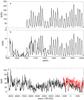 |
Fig. 1 Wolf sunspot number (WSN, panel a)), group sunspot number (GSN, panel b)), and sunspot number reconstructions (SNR) based on dendrochronologically dated radiocarbon concentrations (panel c)). Black and red lines in panel c) refer to the sunspot number reconstructions obtained by Solanki et al. (SNR04, 2004) and Usoskin et al. (SNR14, 2014), respectively. See the text for details. |
The raw datasets are shown in Fig. 1. In order to investigate time variability of these data, the EMD is applied as follows. Each time series s(t) is decomposed into a finite number m of adaptive basis vectors whose number and functional form depend on the dataset under study: 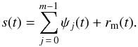 (1)In Eq. (1) s(t) is the raw time series, ψj(t) and rm(t) represent the basis vectors (modes), called intrinsic mode functions (IMF), and the residue, respectively. Each IMF represents a zero mean oscillation with amplitude and phase modulations; it can be written as ψj(t) = Aj(t)cos [φj(t)], where Aj(t) and φj(t) are the amplitude and the phase. IMFs are obtained by following an iterative process based on the identification of the relative maxima and minima from the raw data. An IMF is the result of the average between local maxima and local minima envelopes when it satisfies two properties: (i) the number of extrema and zero-crossings is either equal or differs at most by one and (ii) at any point the mean value of the lower and upper envelopes, formed by the local maxima and the local minima, is zero. The scale of variations described by each IMF is then fixed by the sequence of the local extrema. Further details about the iterative process used to calculate the IMFs can be found in Vecchio et al. (2012a) and Laurenza et al. (2012). The residue rm(t) in Eq. (1) describes the mean trend, when present. The statistical significance of the IMFs is checked by using the test developed by Wu & Huang (2004) and based on the comparison between the IMFs obtained from the signal with those derived from a white-noise process. This approach represents the analogy of the statistical significance tests used in other common decomposition techniques; for instance, as far as the wavelet power spectrum is concerned, theoretical wavelet spectra for white- or red-noise processes are derived and used to establish significance levels and confidence intervals. The decomposition through IMFs defines a meaningful instantaneous frequency for each ψj, calculated by first applying the Hilbert transform
 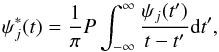 (2)where P indicates the Cauchy principal value, and then calculating the instantaneous phase
 ![Mathematical equation: \hbox{$\phi_j(t)=\arctan[\psi^{*}_j(t)/{\psi_j(t)}]$}](/articles/aa/full_html/2017/03/aa29758-16/aa29758-16-eq46.png) , since ψj(t) and
, since ψj(t) and  form the complex conjugate pair. The instantaneous frequency follows as ωj(t) = dφj/ dt and the instantaneous amplitude is
 ![Mathematical equation: \hbox{$A(t)=[\psi_j^2+\psi_j^{*2}]^{1/2}$}](/articles/aa/full_html/2017/03/aa29758-16/aa29758-16-eq49.png) . A typical timescale τj can be computed for each IMF as τj = (2π)/ ⟨ ωj(t) ⟩, where ⟨·⟩ denotes time averages. We note that τj cannot be interpreted as the period of a Fourier mode because it only provides an estimate of the timescale characterizing an EMD mode; therefore, many modes with different average periods may contribute to the variability of the actual signal at a given timescale. The τj uncertainty is calculated as (2π)/ ⟨ ωj(t) ⟩ 2Δω, where Δω is the standard deviation of each instantaneous frequency. Moreover, the robustness of the period estimated for each EMD oscillation is verified through the following approach. For each sunspot time series s(t) we build up a sample of 1000 new realizations, by making use of the uncertainty σs(t) available for each dataset, as
. A typical timescale τj can be computed for each IMF as τj = (2π)/ ⟨ ωj(t) ⟩, where ⟨·⟩ denotes time averages. We note that τj cannot be interpreted as the period of a Fourier mode because it only provides an estimate of the timescale characterizing an EMD mode; therefore, many modes with different average periods may contribute to the variability of the actual signal at a given timescale. The τj uncertainty is calculated as (2π)/ ⟨ ωj(t) ⟩ 2Δω, where Δω is the standard deviation of each instantaneous frequency. Moreover, the robustness of the period estimated for each EMD oscillation is verified through the following approach. For each sunspot time series s(t) we build up a sample of 1000 new realizations, by making use of the uncertainty σs(t) available for each dataset, as  (3)where βk(t) represents a random number series from a normal distribution with zero mean and unit standard deviation. The EMD method is applied to each sk(t) and the periods of the corresponding IMFs are calculated. In this way we are able to evaluate the dispersion of the obtained periods from the sample of 1000 realizations and, thus, to evaluate a confidence interval Δτj for the period τj.
The EMD decomposition is local, complete, and orthogonal (Huang et al. 1998; Cummings et al. 2004). These properties allow us to filter and reconstruct the signal through partial sums in Eq. (1) in order to obtain independent contributions to the original signal in different ranges of timescales (Huang et al. 1998; Terradas et al. 2004; Vecchio et al. 2012a; Alberti et al. 2014). We note that the observed solar activity variations are far from being stationary periodic fluctuations; thus, methods based on Fourier transforms or periodograms only give partial information on the nature of the solar variability. Moreover, since the EMD describes a signal in terms of empirical time-dependent amplitude and phase functions, it overcomes some limitations of methods based on fixed basis functions such as Fourier and wavelet analysis, thus allowing a correct description of nonlinearities and nonstationarities (Huang et al. 1998). Since the scale of variability of the EMD modes is given by the sequence of the local maxima/minima in the data, our approach retraces the early works of Wolf (1861) and Gleissberg (1971) and, more recently, Richard (2004) who tried to recognize long-term variations from the sequence of local maxima in the data.
3. Results for WSN and GSN
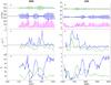 |
Fig. 2 Comparison between the two sunspot number datasets, Wolf sunspot number (WSN) and group sunspot number (GSN), and the respective empirical mode decomposition results for modes j = 1,2. Panels a), b): WSN and GSN data (magenta) and intrinsic mode functions ψ1 (blue) and ψ2 (green) for WSN and GSN data. ψ1 and ψ2 are offset from the zero value by 350, 600 for WSN and 25, 45 for GSN. Panels c), d): instantaneous frequencies ω1 (blue) and ω2 (green) of the j = 1,2 modes for WSN and GSN data. The horizontal black dashed line indicates the 11 yr frequency. Panels d), e): instantaneous amplitudes A1 (blue) and A2 (green) of the j = 1,2 modes for WSN and GSN data. |
In order to fix some constraints for interpretation of the long SNR series, we start the analysis on the WSN and GSN sunspot records. When the EMD is used to analyze WSN and GSN datasets, m = 8 IMFs are obtained for both.
Characteristics of the intrinsic mode functions for the Wolf sunspot number (WSN) and group sunspot number (GSN) datasets.
In Table 1 the following information is listed: the number m; the mean square amplitude Ej (quantifying the mode “energy”, i.e., the contribution of each IMF to the global variability), defined as  (4)the typical period τj; and the 95% confidence interval Δτj for each period, obtained from the 1000 realizations.
For both datasets the highest amplitude IMF is j = 1 (τ1 ~ 9 yr) and it is followed, in decreasing energy order, by mode j = 2 (τ2 ~ 14 yr). These modes together contribute about 70% of the total variance of the signal. Both IMFs compose the Schwabe cycle, which has been observed to have variable periods from 8 to 14 yr (Eddy 1976; Fligge et al. 1999). In Fig. 2 (panels a, b) IMFs j = 1,2 are compared with the raw data for both WSN and GSN. Panels c, d show the instantaneous frequencies for the same modes and the instantaneous amplitudes are displayed in panels e, f. IMF ψ1 (blue lines in panels a and b) clearly reflects the main Schwabe cycle evolution and the corresponding instantaneous frequency variates around Ω0 = 2π/ 11 yr-1 (dashed line in panels c, d of Fig. 2). For both WSN and GSN, the ψ1 amplitude decreases around year 1800 in correspondence with the Dalton minimum and the associated instantaneous frequency departs from Ω0. In the same interval, the ψ2 amplitude increases and ω2 is closer to Ω0, although smaller, thus indicating that the WSN and GSN variability at this time is mainly described by IMF j = 2 (green line). Since the EMD is very sensitive to local frequency changes, the fact that the Schwabe cycle is described by two IMFs suggests that during the grand minima the cycle period changes slightly. Evidence of varying periods of the Schwabe cycle during grand minima states are reported in the literature (see, e.g., Fligge et al. 1999; Usoskin & Mursula 2003). It can also be noted that the behavior of the two IMFs describing the Schwabe cycle appears to be compatible with the known inverse correlation between rise time and amplitude of the cycle (known as the Waldmeier effect), which has been shown to be connected to the periodicity variations observed around grand minima (Petrovay 2010a). The WSN ψ1 shows a similar amplitude decrease around 1900, between cycles 13 and 14, although this feature is less evident in the GSN data. The change of ψ1 for WSN is clearly highlighted by the instantaneous frequency and amplitude which follow an evolution similar to those observed for the Dalton minimum. We note that for GSN, A1(t) shows a relative minimum around 1900 even if no relevant frequency changes are observed. Actually, for cycle 14, the sunspot areas have been observed to have the lowest maximum values in the last 100 yr, which was attributed to a decreased strength of the polar fields during their preceding solar cycle (Diego et al. 2010). Indeed, according to some dynamo models (e.g., Dikpati et al. 2004; Choudhuri 2008), the polar field is essential for the generation of sunspots of the subsequent cycle.
The time behavior at the Maunder minimum, encompassed only by GSN, is more complex. At the beginning of the minimum, the main scale of variability is 11 yr since IMF j = 1 has a higher amplitude than j = 2. In the deep minimum both j = 1,2 modes show a very low amplitude. Toward the end of the minimum, the solar activity recovery, mainly described by ψ2, occurs at timescales slightly longer than those of ψ1.
For both WSN and GSN, IMFs having low Ej can be associated with other well-known periodicities detected in the solar activity: ψ0 with quasi-biennial oscillations (QBOs; Vecchio et al. 2010; Laurenza et al. 2012; Vecchio et al. 2012b; Bazilevskaya et al. 2014); ψ3,ψ4 with the Hale 22 yr cycle. In particular, as for the Schwabe cycle, the 22 yr mode of variability is separated into two IMFs, indicating that during the Maunder minimum its period changes slightly (Inceoglu et al. 2015). It can be seen in Fig. 3 that around the Maunder minimum for the GSN, ψ4 amplitude is higher than the ψ3 value, indicating that the Hale cycle occurs at a slightly higher period (~ 27 yr). For WSN, starting from about year 1800, ψ3 amplitude remains higher than ψ4, except for a short interval around 1900. On the other hand, the two amplitudes are almost comparable around 1900 in the GSN dataset.
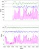 |
Fig. 3 Sunspot number data (magenta) for the two considered datasets and respective intrinsic mode functions ψ3 (blue) and ψ4 (green) obtained from their empirical mode decomposition. Panel a): wolf sunspot number (WSN). Panel b): group sunspot number (GSN). ψ3 and ψ4 are offset from the zero value by 250, 320 for WSN and 15, 30 for GSN. |
Empirical modes j = 5,6, with typical periods between 70 and 130 yr, can be associated with the Gleissberg cycle, commonly detected at timescales in the range 55−120 yr (Usoskin 2013; Petrovay 2010b). For WSN and GSN τj values are slightly different but compatible within uncertainties. IMFs ψ7 could be related to the ~ 200 yr Suess supersecular cycle that is discussed in detail in the next section. Figure 4 shows IMFs j = 5−7 for both WSN and GSN (panels a and b, respectively). The occurrence of two IMFs associated with the Gleissberg cycle suggests that it could be made by multiple branches at different scales of variability. This is in agreement with Ogurtsov et al. (2002), who suggested that this solar cycle oscillation has a double structure consisting of two distinct scales around 50−80 and 90−140 yr. We note that approaches suggesting that the Gleissberg cycle could be made by a single oscillation of varying period in time (e.g., Kolláth & Oláh 2009), mainly based on Fourier and wavelet-based analysis, could be biased by the combination of non-adaptive techniques, poor frequency sample, and shortness of the observed sunspot datasets providing solutions in which the oscillating modes are mixed together, while actually distinct oscillations are present. Indeed, the use of fixed basis functions, which in a nonstationary case are far from being eigenfunctions of the phenomenon at hand, with short (with respect to the oscillation wavelength) datasets can provide a solution where modes are mixed together in such a way that the solution is compatible with the fictitious conditions imposed by the analysis. On the other hand, in these situations an empirical decomposition such as the EMD allows a better description of the nonstationarities and it does not introduce, unlike Fourier analysis, spurious harmonics in reproducing nonstationary data and nonlinear waveform deformations.
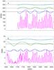 |
Fig. 4 Sunspot number data (magenta) for the two considered datasets and respective intrinsic mode functions ψ5 (blue), ψ6 (green), and ψ7 (light blue) obtained from their empirical mode decomposition. Panel a): Wolf sunspot number (WSN). Panel b): group sunspot number (GSN). ψ5, ψ6, and ψ7 are offset from the zero value by 250, 300, and 350 for WSN and 12, 18, and 22 for GSN. |
For both datasets, ψ5 underlines the Dalton minimum and the activity decrease around 1900, and for the WSN dataset it has higher Ej than ψ6 and ψ7. The same occurs for GSN data when reduced to the same WSN time interval 1700−2014 (not shown). On the other hand, for the full GSN Ej is larger for ψ6, thus indicating, as clearly shown in Fig. 4, that the activity variations related to the two grand minima present in the data are encompassed by this mode. IMF j = 7, describing slower variations of the sunspot dynamics, has minima at the Maunder decrease and around 1900. According to these results, the sequence of the Maunder and Dalton minima in the sunspot variability is produced by the variations due to long period contributions. In the following, we will extend our analysis to the longer SNR dataset by using the results obtained for WSN and GSN data with τj> 40 yr as a term of comparison.
4. Results for SNR
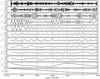 |
Fig. 5 Empirical mode decomposition modes ψj and the residue rm(t) for the sunspot number SNR04 dataset (Solanki et al. 2004). |
Concerning SNR data, 11 and 8 IMFs have been found for SNR04 (shown in Fig. 5) and SNR14, respectively. Table 2 shows the Ej, τj, and the 95% confidence interval Δτj of each EMD period for both the SNR datasets.
Characteristics of the intrinsic mode functions for the sunspot number SNR04 (Solanki et al. 2004) and SNR14 (Usoskin et al. 2014) datasets.
To evaluate the reliability of the modes related to the Gleissberg cycle, we compare the IMFs previously obtained for WSN and GSN with those from SNR. Because of the different sampling time (1 yr for WSN/GSN and 10 yr for SNR) we compare WSN/GSN modes j = 5−7 with SNR modes j = 0−2 in the time interval 1600−2014 (Fig. 6).
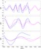 |
Fig. 6 Comparison between EMD modes with similar timescales from different data. Panel a): intrinsic mode function (IMF) ψ5 for Wolf sunspot number (WSN, magenta dashed) and group sunspot number (GSN, magenta full), IMF ψ0 for sunspot numbers SNR04 (blue) and SNR14 (blue dot-dashed). Panel b): IMF ψ6 for WSN (magenta dashed) and GSN (magenta full), IMF ψ1 for SNR04 (blue) and SNR14 (blue dot-dashed). Panel c): IMF ψ7 for WSN (magenta dashed) and GSN (magenta full), IMF ψ2 for SNR04 (blue) and SNR14 (blue dot-dashed). For panels a) and b), the WSN and GSN IMFs are divided and multiplied by the same factor 5 and the SNR14 IMF is divided by 2; for panel c), the WSN IMF is divided by 2, the GSN IMF is multiplied by 8 and the SNR14 IMF is divided by 5. |
The phasing and the periods of the IMFs, as obtained from the three datasets, agree quite closely; the small discrepancies are probably due to the different sampling among the datasets. We also note the different behavior of the SNR14 ψ0 (blue dot-dashed line in panel a of Fig. 6) around 1850 with respect to the same IMF from the other records, indicating that the SNR14 record, at timescales around 40 yr, behaves differently from the three other datasets. Since this record has been derived by using the most recent models of Earth’s dipole and 14C production rate, further investigation could explain whether the observed differences are real or simply arise from some features in the models. Although derived in a time interval that is short with respect to the typical period (~ 200 yr), the WSN/GSN j = 7 mode also shows a similar time behavior to the j = 2 SNR IMFs. This simple test indicates that modes extracted through the EMD from three independent datasets are reliable since nearly the same time variability is recovered.
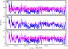 |
Fig. 7 Empirical mode decomposition reconstructions (magenta lines) superimposed to the sunspot number SNR04 dataset (blue lines). The shown reconstructions are obtained by summing up modes j = 0−2 (panel a)), j = 3,4 (panel b)), and j = 0−4 (panel c)) and by adding an offset of 40. |
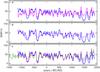 |
Fig. 8 Empirical mode decomposition reconstructions (magenta lines) superimposed to the sunspot number SNR14 dataset (blue lines). The shown reconstructions are obtained by summing up modes j = 0−3 (panel a)), j = 4,5 (panel b)), and j = 0−5 (panel c)) and by adding an offset of 40. The green line in panel c) refers to the SNR04 reconstruction through IMFs j = 0−4. |
The above comparison is useful in order to interpret the results from the SNR dataset. SNR04 IMFs j = 0,1 are clearly associated with the two modes of the Gleissberg cycle already mentioned in the previous section. IMF j = 2 describes the same phenomenon of the mode j = 7 of WSN/GSN and its period, τ2 ~ 150 yr, falls into the typical range of the Gleissberg cycle. Since they are calculated from a longer dataset, we believe that the periods calculated from SNR are more representative than those calculated from WSN/GSN. SNR results indicate that the Gleissberg cycle is split into more than two IMFs, i.e., several branches contribute to this periodicity. The sum of these modes, which accounts for ~ 40% of the total variance, describes the total Gleissberg cycle. These results suggest that IMF j = 7 from WSN/GSN could be the third IMF contributing to the Gleissberg cycle. SNR04 IMF j = 3, accounting for 16% of the total variance of the signal, can be associated with the Suess oscillation and mode j = 4, accounting for ~ 13% of the total variance, could be associated with the unnamed cycle detected with a period of around 350 yr claimed by Steinhilber et al. (2012). Nevertheless, this IMF has a similar temporal evolution of ψ3, namely the intervals of high and low amplitude are almost coincident (see Fig. 5), thus suggesting that, as is true for the Gleissberg cycle, the Suess oscillation could also be split into more than one IMF.
Since the two SNR datasets are recorded in different periods, we also apply the EMD technique to the SNR04 reduced to the same length as SNR14. Corresponding Ej and τj are shown in parentheses in Table 2. A one-to-one correspondence between reduced SNR04 and SNR14 IMFs is not observed. Modes j = 0,1 from the two datasets are characterized by similar Ej and τj. On the other hand, the reduced SNR04 τ2 is between the SNR14 τ2 and τ3. Comparable τj are observed for reduced SNR04 j = 3,4 and SNR14 j = 4,5. Differences in the observed timescales can be due to local differences in the two SNR datasets resulting in different IMF sequences. Very similar time evolutions of the reduced SNR04 mode j = 2 to the sum of modes j = 2,3 of the SNR14 dataset indicate that the latter can be reasonably associated with the Gleissberg cycle (similar time behavior is also observed when the full Gleissberg contributions, j = 0,2 for SNR04 and j = 0,3 of the reduced SNR14 are compared). This interpretation is also consistent with the IMF energy content: the sum E2 + E3 = 37% for SNR14 is comparable with E2 for the reduced SNR04. We note that by comparing the SNR14 and reduced SNR04 datasets the Suess contribution is ~ 28% (E4 + E5) for the former and ~ 26% (E3 + E4) for the latter. By following these considerations, we considered the Gleissberg cycle, for the SNR14 data, to be described by the sum of the modes 0−3, and the Suess cycle by the modes 4−5.
The EMD partial reconstructions of the Gleissberg and Suess oscillations (ψ0 + ψ1 + ψ2 and ψ3 + ψ4, respectively) for the full SNR04 dataset are shown in panels a,b of Fig. 7. Panel c, illustrates the EMD reconstruction j = 0−4 (Gleissberg+Suess), superimposed to the raw data. This reconstruction reproduces the sequence of maxima and minima observed in the raw data, indicating that the grand minima are traced by variations at typical timescales of Gleissberg and Suess oscillations. The Gleissberg and Suess oscillations (ψ0 + ψ1 + ψ2 + ψ3 and ψ4 + ψ5, respectively) and their sum for SNR14 are shown in Fig. 8. For both SNR data, the Gleissberg cycle (panels a) reproduces the majority of the relative minima of the raw signal, whereas the Suess cycle (panels b) traces the occurrence of the high amplitude minima. The combination of both cycles (panels c) follows the general oscillating trend of the data and explains the majority of the grand minima. This is in agreement with the findings of Steinhilber et al. (2012), who observed via a wavelet analysis on the total solar irradiance that the grand solar minima preferentially occur at the minima of the Suess cycle.
High j values, at typical timescales between ~ 600 and ~ 2400 yr, are characterized by lower Ej than Gleissberg and Suess associated modes. We note that these timescales were also detected when wavelet analysis was used to analyze 14C records (Steinhilber et al. 2012). In particular, modes j = 9 and j = 7 of SNR04 and SNR14, respectively, could be associated with the Hallstatt cycle, likely related to solar activity (Usoskin et al. 2016). IMF j = 10 of SNR04, accounting for 17.8% of the total energy, represents a very long modulation scale causing, for example, the general decrease in the SNR04 between 6000 and 5000 BC. This decrease is not accounted for by the reconstruction with the Gleissberg and Suess modes (panel c of Fig. 7). The ψ10 behavior is very close to the non-solar long-term component found by Usoskin et al. (2016) associated with 14C transport and deposition effects at the Earth.
In the following we focus on the IMFs associated with the Gleissberg and Suess cycles by discussing their relationship with the solar minima occurrence.
5. Occurrence of grand minima
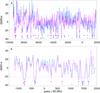 |
Fig. 9 Sunspot number (blue line) for the two datasets SNR04 (panel a)) and SNR14 (panel b)) and respective empirical mode decomposition (magenta line) reconstructions through modes j = 1−4 (panel a)) and j = 1−5 (panel b)). Horizontal magenta lines indicate the 90th percentile of the EMD reconstruction distribution function. Magenta dots correspond to times when the EMD reconstructions (magenta lines) are beyond the 90th percentile of its distribution function. Blue dots mark grand minima also occurring in a relative minima of the Suess cycle (j = 3,4 for SNR04 and j = 4,5 for SNR14) exceeding the 90th percentile of the distribution function of this signal. Black asterisks correspond to the grand minima identified in Usoskin et al. (2007). |
As shown in the previous section the occurrence of grand minima is described by the coupling between the Gleissberg and Suess cycles. Grand minima, representing strong decreases in SNR timeseries, strongly contribute to the signal variance. Hence, we introduce a novel criterion to identify grand minima through sunspot signals obtained only with the highest energy and longest period Gleissberg and Suess contributions (i.e., the sum of ψ1−ψ4 for SNR04 and ψ1−ψ5 for SNR14). A relative minimum of this signal is considered to be a grand minimum if it is beyond the 90th percentile of the signal distribution function (horizontal magenta line in panels a and b of Fig. 9). The magenta dots in Fig. 9 show the times when this condition is fulfilled. By using this approach, 27 grand minima have been identified in SNR04 datasets mostly coincident with the grand minima independently identified by Usoskin et al. (2007), Inceoglu et al. (2015), Usoskin et al. (2016). The duration of the detected grand minima, calculated as the length of the time interval at 90% of the lowest value, is shown in Table 3. Our approach, able to isolate the Gleissberg and Suess cycles by excluding other contributions, allows an evaluation of the grand minima that is not biased by the presence of non-solar long-term modulations (which can locally produce an increase/decrease in the 14C sunspot data). For example, we do not identify any grand minima in the period 6000−5000 BC corresponding to the minimum of the large-scale ~ 7000 yr IMF j = 10. If not correctly filtered, this oscillation can bias the grand minima identification obtained by making use of threshold criteria applied on the raw signal.
The blue dots in Fig. 9 indicate the previously identified grand minima which also occur in a relative minimum of the Suess cycle (sum of the SNR04 modes j = 3,4 and SNR14 modes j = 4,5), exceeding the 90th percentile of the distribution function of this signal. We note that these grand minima are longer, being characterized by a duration of more than 90 yr (asterisks in Table 3), where the only exception is the minimum at 6415 BC lasting 90 yr but not occurring at a Suess cycle minimum. Our interpretation of grand minima in terms of interference between solar variability cycles allows a possible explanation for the origin of the two expected distinct types of grand minima: shorter Maunder-type and longer Spörer-like minima (Stuiver & Braziunas 1989). While the grand minima sequence is produced by the coupling between Gleissberg and Suess cycles, the latter is mainly responsible for the Spörer-like minima having longer duration.
Time of occurrence and duration of the grand minima in − BC/AD.
To evaluate the relative contribution of the Gleissberg and Suess cycles to the minima intensity we show in panel a of Fig. 10 the scatter plot of the amplitude of the single Suess (purple dots) and Gleissberg cycles (green dots) at grand minima as a function of their sum at the same times. It can be seen that the deepest grand minima, having global amplitudes of less than −23 are the most intense and occur mainly at large negative amplitudes of the Suess cycle. Moreover, as shown in panel b of Fig. 10, the long-lasting minima, associated with the Suess cycle (marked with an asterisks in Table 3), tend to have the largest negative amplitude. The only exception is represented by the Maunder minimum which, despite a short duration, has a large negative amplitude. These findings are in agreement with the observed tendency for intense minima to last longer than moderate activity period (Inceoglu et al. 2015).
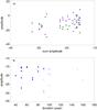 |
Fig. 10 Panel a): amplitude of the Gleissberg (green dots) and Suess (purple dots) cycles, reconstructed through the empirical mode decomposition (see text for details), at grand minima as a function of the amplitude of their sum at the same times. Panel b): grand minima amplitudes as a function of their duration. Asterisks indicate grand minima occurring at a minimum of the Suess cycle. |
Figure 11 shows the time behavior of the IMF ψ9, associated with the Hallstatt cycle, and the times of the detected grand minima. No clear relationship between maxima and minima of this cycle and the grand minima occurrence is detected. Indeed, while Hallstatt cycle minima around −5300 BC and −1300 BC correspond to voids in the grand minima sequence, the remaining minima (around −8100 BC, −3200 BC, and 1300 AD) coincide with minima occurrence. We note that these findings are slightly different from the results of Clilverd et al. (2003) and Usoskin et al. (2016) who found that grand minima tend to cluster around the minima of the Halstatt cycle. Differences can result from both the different definition of grand minima used in the present paper and the way through which non-solar long-period contributions are filtered out from the raw data, both based on the EMD technique. This point deserves further investigation in the future.
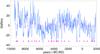 |
Fig. 11 Intrinsic mode function ψ9 (magenta line), associated with the Hallstatt cycle, superimposed onto the sunspot number SNR04 dataset (blue line). Magenta dots correspond to the grand minima identified in this paper. |
6. Conclusions
The EMD technique was used to analyze the novel yearly average of WSN and GSN, and two SNR datasets at decadal resolution. This approach allowed us to investigate the long-term time variability and the grand minima occurrence in all the datasets. The main results are summarized as follows.
6.1. Schwabe and Hale cycle
For WSN and GSN datasets the two highest energy modes are associated with the Schwabe cycle. The EMD derived instantaneous frequencies and amplitudes for these modes indicate that this cycle, during the Maunder and Dalton minima, occurs on a longer timescale of about 14 yr (Fligge et al. 1999; Usoskin & Mursula 2003; Petrovay 2010a). This behavior is in agreement with the well-known inverse proportionality between cycle rise time and amplitude (Waldmeier effect; Petrovay 2010a). In the WSN data around 1900, between cycles 13−14, IMFs associated with the Schwabe cycle show a behavior similar to that observed in the Maunder and Dalton minima, thus suggesting a minimum-like behavior.
Low energy IMFs have been associated with the well-known periodicities detected in the solar activity, such as the QBOs and the Hale cycle. As for the Schwabe cycle, the 22 yr mode of variability is separated into two IMFs indicating that during the Maunder minimum this period slightly changes.
6.2. Gleissberg and Suess cycles
Two IMFs at timescales between 70−130 yr have been found in WSN and GSN data. These modes have been attributed to the Gleissberg cycle. Finally, for both datasets, a unique IMF at a timescale of ~ 200 yr has been found. Our results underline that the Gleissberg cycle causes the activity variations giving rise to the Maunder and Dalton minima, indicating that it plays a relevant role in the solar minima generation.
A direct comparison between SNR and WSN/GSN IMFs shows that the EMD results are reliable since the same scales of variability and similar time behaviors are independently found in the four datasets. When applied to the SNR datasets the EMD is able to efficiently identify a non-solar component: a very long scale oscillation (~ 7000 yr) containing about 18% of the total variance of the signal and significantly affecting the time behavior of the SNR04 data. Moreover, the Hallstatt cycle, likely related to the solar activity, has been detected. The most energetic modes for both SNRs are associated with the Gleissberg and Suess cycles. A deeper characterization of the Gleissberg and Suess cycles is possible owing to the long duration of SNR datasets with respect to WSN/GSN ones. Our findings indicate that the Gleissberg cycle, often identified with a single oscillation of varying period in time, and the Suess cycle are actually composed of a multibranch structure at distinct scales of oscillations (Ogurtsov et al. 2002; Usoskin 2013). We verified that the Gleissberg and Suess cycles, containing most of the signal energy, are strongly involved in the grand minima generation. Hence a new approach, which only takes into account the contribution of these cycles and excluding, for instance, modulations due to terrestrial effects, has been proposed to identify and characterize the grand minima. We found that coupling between the Gleissberg and Suess cycles mostly defines the time sequence of the grand minima. In addition, grand minima occurring at a minimum of the Suess cycle are found to be the most intense and the longest (with typical duration longer than 80 yr). In other words, the Suess cycle represents the variability timescale of the Spörer-like minima.
Concerning the time behavior of the grand minima occurrence, although the MHD dynamo is a deterministic process, we note that it can give rise to grand minima events irregularly distributed in time (Weiss et al. 1984; Moss et al. 2008; Usoskin et al. 2009; Petrovay 2007). Our results suggest that the occurrence of grand minima is a consequence of the complex superposition of systematic long-term activity cycles and seems not to be a random process, as proposed in earlier works (Usoskin et al. 2014, 2016; Inceoglu et al. 2015).
We note that the characterization of secular cycles of solar activity and the grand minima occurrence, generation, and their possible regular or chaotic behavior is important for a deeper understanding of the solar dynamo process. Indeed, although long-term modulations of the basic 11 yr cycle have been produced in the framework of nonlinear α−ω dynamo models (Tobias 1996, 1997) and the 2D model of a distributed dynamo (Pipin 1999), the physical mechanisms underlying their occurrence are still unknown mainly owing to simplifying assumptions used in the models. New observations and deeper characterizations of the long-term activity are thus required to provide more constraints to build up theoretical models able to take into account the many physical aspects involved in the solar dynamo. We also remark that a deep characterization of long-term cycles in the Sun is also important in the framework of the investigation of stellar activity. For instance, Saar & Brandenburg (1999), by comparing observations with the results of a dynamo model, showed that the Gleissberg cycle is also present for a large stellar population.
Acknowledgments
M.L. and V.C acknowledge support by the Italian Ministry for Education and Research MIUR PRIN Grant No. 2012P2HRCR on “The active Sun and its effects on Space and Earth climate”. We thank the anonymous reviewer for fruitful suggestions.
References
- Alberti, T., Lepreti, F., Vecchio, A., et al. 2014, Climate of the Past, 10, 1751 [Google Scholar]
- Attolini, M. R., Cecchini, S., Galli, M., & Nanni, T. 1987, International Cosmic Ray Conference, 4, 323 [NASA ADS] [Google Scholar]
- Attolini, M. R., Cecchini, S., Nanni, T., & Galli, M. 1990, Sol. Phys., 125, 389 [NASA ADS] [CrossRef] [Google Scholar]
- Bazilevskaya, G., Broomhall, A.-M., Elsworth, Y., & Nakariakov, V. M. 2014, Space Sci. Rev., 186, 359 [NASA ADS] [CrossRef] [Google Scholar]
- Beer, J., Siegenthaler, U., Oeschger, H., Bonani, G., & Finkel, R. C. 1988, Nature, 331, 675 [NASA ADS] [CrossRef] [Google Scholar]
- Choudhuri, A. R. 2008, J. Astrophys. Astron., 29, 41 [NASA ADS] [CrossRef] [Google Scholar]
- Cini Castagnoli, G., Bonino, G. S. M., & P., S. C. 1992, Radiocarbon, 34, 798 [CrossRef] [Google Scholar]
- Clette, F., Svalgaard, L., Vaquero, J. M., & Cliver, E. W. 2014, Space Sci. Rev., 186, 35 [NASA ADS] [CrossRef] [Google Scholar]
- Clilverd, M. A., Clarke, E., Rishbeth, H., Clark, T. D. G., & Ulich, T. 2003, Astron. Geophys., 44, 5.20 [CrossRef] [Google Scholar]
- Cummings, D. A. T., Irizarry, R. A., Huang, N. E., et al. 2004, Nature, 427, 344 [NASA ADS] [CrossRef] [PubMed] [Google Scholar]
- Damon, P. E., & Sonett, C. P. 1991, in The Sun in Time, eds. C. P. Sonett, M. S. Giampapa, & M. S. Matthews, 360 [Google Scholar]
- Diego, P., Storini, M., & Laurenza, M. 2010, J. Geophys. Res. (Space Physics), 115, A06103 [NASA ADS] [CrossRef] [Google Scholar]
- Dikpati, M., de Toma, G., Gilman, P. A., Arge, C. N., & White, O. R. 2004, ApJ, 601, 1136 [NASA ADS] [CrossRef] [Google Scholar]
- Eddy, J. A. 1976, Science, 192, 1189 [NASA ADS] [CrossRef] [PubMed] [Google Scholar]
- Feynman, J. 1983, in NASA Conference Publication, 228 [Google Scholar]
- Feynman, J., & Fougere, P. F. 1984, J. Geophys. Res., 89, 3023 [Google Scholar]
- Fligge, M., Solanki, S. K., & Beer, J. 1999, A&A, 346, 313 [NASA ADS] [Google Scholar]
- Frick, P., Galyagin, D., Hoyt, D. V., et al. 1997, A&A, 328, 670 [NASA ADS] [Google Scholar]
- Gleissberg, W. 1958, J. Br. Astron. Assoc., 68, 148 [Google Scholar]
- Gleissberg, W. 1965, J. Br. Astron. Assoc., 75, 227 [Google Scholar]
- Gleissberg, W. 1971, Sol. Phys., 21, 240 [NASA ADS] [CrossRef] [Google Scholar]
- Huang, N. E., Shen, Z., Long, S. R., et al. 1998, Proc. Royal Society of London A: Mathematical, Physical and Engineering Sciences, 454, 903 [Google Scholar]
- Inceoglu, F., Simoniello, R., Knudsen, M. F., et al. 2015, A&A, 577, A20 [NASA ADS] [CrossRef] [EDP Sciences] [Google Scholar]
- Kolláth, Z., & Oláh, K. 2009, A&A, 501, 695 [NASA ADS] [CrossRef] [EDP Sciences] [Google Scholar]
- Laurenza, M., Vecchio, A., Storini, M., & Carbone, V. 2012, ApJ, 749, 167 [Google Scholar]
- Lin, Y. C., Fan, C. Y., Damon, P. E., & Wallick, E. I. 1975, International Cosmic Ray Conference, 3, 995 [NASA ADS] [Google Scholar]
- Link, F. 1963, Bulletin of the Astronomical Institutes of Czechoslovakia, 14, 226 [NASA ADS] [Google Scholar]
- McCracken, K. G., & Beer, J. 2008, International Cosmic Ray Conference, 1, 549 [NASA ADS] [Google Scholar]
- Moss, D., Sokoloff, D., Usoskin, I. G., & Tutubalin, V. 2008, Sol. Phys., 250, 221 [NASA ADS] [CrossRef] [Google Scholar]
- Ogurtsov, M. G., Nagovitsyn, Y. A., Kocharov, G. E., & Jungner, H. 2002, Sol. Phys., 211, 371 [NASA ADS] [CrossRef] [Google Scholar]
- Peristykh, A. N., & Damon, P. E. 2003, J. Geophys. Res. (Space Phys.), 108, 1003 [Google Scholar]
- Petrovay, K. 2007, Astron. Nachr., 328, 777 [NASA ADS] [CrossRef] [Google Scholar]
- Petrovay, K. 2010a, in Solar and Stellar Variability: Impact on Earth and Planets, eds. A. G. Kosovichev, A. H. Andrei, & J.-P. Rozelot, IAU Symp., 264, 150 [Google Scholar]
- Petrovay, K. 2010b, Liv. Rev. Sol. Phys., 7, 6 [Google Scholar]
- Pipin, V. V. 1999, A&A, 346, 295 [NASA ADS] [Google Scholar]
- Raisbeck, G. M., Yiou, F., Jouzel, J., & Petit, J. R. 1990, Philosophical Transactions of the Royal Society of London Series A, 330, 463 [Google Scholar]
- Richard, J.-G. 2004, Sol. Phys., 223, 319 [NASA ADS] [CrossRef] [Google Scholar]
- Saar, S. H., & Brandenburg, A. 1999, ApJ, 524, 295 [NASA ADS] [CrossRef] [Google Scholar]
- Schove, D. J. 1955, J. Geophys. Res., 60, 127 [NASA ADS] [CrossRef] [Google Scholar]
- Solanki, S. K., Usoskin, I. G., Kromer, B., Schüssler, M., & Beer, J. 2004, Nature, 431, 1084 [NASA ADS] [CrossRef] [PubMed] [Google Scholar]
- Sonett, C. P. 1984, Rev. Geophys. Space Phys., 22, 239 [NASA ADS] [CrossRef] [Google Scholar]
- Sonett, C. P., & Finney, S. A. 1990, Philosoph. Trans. Roy. Soc. London Ser. A, 330, 413 [Google Scholar]
- Steinhilber, F., Abreu, J. A., Beer, J., et al. 2012, Proc. National Academy of Science, 109, 5967 [Google Scholar]
- Stuiver, M., & Braziunas, T. F. 1989, Nature, 338, 405 [NASA ADS] [CrossRef] [Google Scholar]
- Stuiver, M., & Braziunas, T. 1993, Holocene, 3(4), 289 [Google Scholar]
- Suess, H. E. 1980, Radiocarbon, 22, 200 [CrossRef] [Google Scholar]
- Terradas, J., Oliver, R., & Ballester, J. L. 2004, ApJ, 614, 435 [NASA ADS] [CrossRef] [Google Scholar]
- Tobias, S. M. 1996, A&A, 307, L21 [NASA ADS] [Google Scholar]
- Tobias, S. M. 1997, A&A, 322, 1007 [NASA ADS] [Google Scholar]
- Usoskin, I. G. 2013, Liv. Rev. Sol. Phys., 10, 1 [Google Scholar]
- Usoskin, I. G., & Mursula, K. 2003, Sol. Phys., 218, 319 [NASA ADS] [CrossRef] [Google Scholar]
- Usoskin, I. G., Solanki, S. K., & Kovaltsov, G. A. 2007, A&A., 471, 301 [NASA ADS] [CrossRef] [EDP Sciences] [Google Scholar]
- Usoskin, I. G., Sokoloff, D., & Moss, D. 2009, Sol. Phys., 254, 345 [Google Scholar]
- Usoskin, I. G., Hulot, G., Gallet, Y., et al. 2014, A&A, 562, L10 [NASA ADS] [CrossRef] [EDP Sciences] [Google Scholar]
- Usoskin, I. G., Gallet, Y., Lopes, F., Kovaltsov, G. A., & Hulot, G. 2016, A&A, 587, A150 [NASA ADS] [CrossRef] [EDP Sciences] [Google Scholar]
- Vecchio, A., Laurenza, M., Carbone, V., & Storini, M. 2010, ApJ, 709, L1 [NASA ADS] [CrossRef] [Google Scholar]
- Vecchio, A., Laurenza, M., Meduri, D., Carbone, V., & Storini, M. 2012a, ApJ, 749, 27 [NASA ADS] [CrossRef] [Google Scholar]
- Vecchio, A., Laurenza, M., Storini, M., & Carbone, V. 2012b, Adv. Astron., 2012, 834247 [Google Scholar]
- Weiss, N. O., Cattaneo, F., & Jones, C. A. 1984, Geophys. Astrophys. Fluid Dyn., 30, 305 [Google Scholar]
- Wolf, R. 1861, MNRAS, 21, 77 [NASA ADS] [Google Scholar]
- Wolf, R. 1862, Astronomische Mitteilungen der Eidgenössischen Sternwarte Zurich, 2, 119 [NASA ADS] [Google Scholar]
- Wu, Z., & Huang, N. E. 2004, Proc. Royal Society of London A: Mathematical, Physical and Engineering Sciences, 460, 1597 [Google Scholar]
All Tables
Characteristics of the intrinsic mode functions for the Wolf sunspot number (WSN) and group sunspot number (GSN) datasets.
Characteristics of the intrinsic mode functions for the sunspot number SNR04 (Solanki et al. 2004) and SNR14 (Usoskin et al. 2014) datasets.
All Figures
|
Fig. 1 Wolf sunspot number (WSN, panel a)), group sunspot number (GSN, panel b)), and sunspot number reconstructions (SNR) based on dendrochronologically dated radiocarbon concentrations (panel c)). Black and red lines in panel c) refer to the sunspot number reconstructions obtained by Solanki et al. (SNR04, 2004) and Usoskin et al. (SNR14, 2014), respectively. See the text for details. |
| In the text | |
|
Fig. 2 Comparison between the two sunspot number datasets, Wolf sunspot number (WSN) and group sunspot number (GSN), and the respective empirical mode decomposition results for modes j = 1,2. Panels a), b): WSN and GSN data (magenta) and intrinsic mode functions ψ1 (blue) and ψ2 (green) for WSN and GSN data. ψ1 and ψ2 are offset from the zero value by 350, 600 for WSN and 25, 45 for GSN. Panels c), d): instantaneous frequencies ω1 (blue) and ω2 (green) of the j = 1,2 modes for WSN and GSN data. The horizontal black dashed line indicates the 11 yr frequency. Panels d), e): instantaneous amplitudes A1 (blue) and A2 (green) of the j = 1,2 modes for WSN and GSN data. |
| In the text | |
|
Fig. 3 Sunspot number data (magenta) for the two considered datasets and respective intrinsic mode functions ψ3 (blue) and ψ4 (green) obtained from their empirical mode decomposition. Panel a): wolf sunspot number (WSN). Panel b): group sunspot number (GSN). ψ3 and ψ4 are offset from the zero value by 250, 320 for WSN and 15, 30 for GSN. |
| In the text | |
|
Fig. 4 Sunspot number data (magenta) for the two considered datasets and respective intrinsic mode functions ψ5 (blue), ψ6 (green), and ψ7 (light blue) obtained from their empirical mode decomposition. Panel a): Wolf sunspot number (WSN). Panel b): group sunspot number (GSN). ψ5, ψ6, and ψ7 are offset from the zero value by 250, 300, and 350 for WSN and 12, 18, and 22 for GSN. |
| In the text | |
|
Fig. 5 Empirical mode decomposition modes ψj and the residue rm(t) for the sunspot number SNR04 dataset (Solanki et al. 2004). |
| In the text | |
|
Fig. 6 Comparison between EMD modes with similar timescales from different data. Panel a): intrinsic mode function (IMF) ψ5 for Wolf sunspot number (WSN, magenta dashed) and group sunspot number (GSN, magenta full), IMF ψ0 for sunspot numbers SNR04 (blue) and SNR14 (blue dot-dashed). Panel b): IMF ψ6 for WSN (magenta dashed) and GSN (magenta full), IMF ψ1 for SNR04 (blue) and SNR14 (blue dot-dashed). Panel c): IMF ψ7 for WSN (magenta dashed) and GSN (magenta full), IMF ψ2 for SNR04 (blue) and SNR14 (blue dot-dashed). For panels a) and b), the WSN and GSN IMFs are divided and multiplied by the same factor 5 and the SNR14 IMF is divided by 2; for panel c), the WSN IMF is divided by 2, the GSN IMF is multiplied by 8 and the SNR14 IMF is divided by 5. |
| In the text | |
|
Fig. 7 Empirical mode decomposition reconstructions (magenta lines) superimposed to the sunspot number SNR04 dataset (blue lines). The shown reconstructions are obtained by summing up modes j = 0−2 (panel a)), j = 3,4 (panel b)), and j = 0−4 (panel c)) and by adding an offset of 40. |
| In the text | |
|
Fig. 8 Empirical mode decomposition reconstructions (magenta lines) superimposed to the sunspot number SNR14 dataset (blue lines). The shown reconstructions are obtained by summing up modes j = 0−3 (panel a)), j = 4,5 (panel b)), and j = 0−5 (panel c)) and by adding an offset of 40. The green line in panel c) refers to the SNR04 reconstruction through IMFs j = 0−4. |
| In the text | |
|
Fig. 9 Sunspot number (blue line) for the two datasets SNR04 (panel a)) and SNR14 (panel b)) and respective empirical mode decomposition (magenta line) reconstructions through modes j = 1−4 (panel a)) and j = 1−5 (panel b)). Horizontal magenta lines indicate the 90th percentile of the EMD reconstruction distribution function. Magenta dots correspond to times when the EMD reconstructions (magenta lines) are beyond the 90th percentile of its distribution function. Blue dots mark grand minima also occurring in a relative minima of the Suess cycle (j = 3,4 for SNR04 and j = 4,5 for SNR14) exceeding the 90th percentile of the distribution function of this signal. Black asterisks correspond to the grand minima identified in Usoskin et al. (2007). |
| In the text | |
|
Fig. 10 Panel a): amplitude of the Gleissberg (green dots) and Suess (purple dots) cycles, reconstructed through the empirical mode decomposition (see text for details), at grand minima as a function of the amplitude of their sum at the same times. Panel b): grand minima amplitudes as a function of their duration. Asterisks indicate grand minima occurring at a minimum of the Suess cycle. |
| In the text | |
|
Fig. 11 Intrinsic mode function ψ9 (magenta line), associated with the Hallstatt cycle, superimposed onto the sunspot number SNR04 dataset (blue line). Magenta dots correspond to the grand minima identified in this paper. |
| In the text | |
Current usage metrics show cumulative count of Article Views (full-text article views including HTML views, PDF and ePub downloads, according to the available data) and Abstracts Views on Vision4Press platform.
Data correspond to usage on the plateform after 2015. The current usage metrics is available 48-96 hours after online publication and is updated daily on week days.
Initial download of the metrics may take a while.