© ESO, 2017

1. Introduction

Babcock (1961) proposed a scenario describing the cyclic solar dynamo in terms of a consistent physical approach based on observational results. These were basically the (latitudinal) differential rotation, the polarity rules of sunspot groups and their systematic tilt with respect to the east-west direction, the reversals of the global dipole field in the course of the solar cycle together with the relationship between its orientation and the sunspot polarities. In Babcock’s scenario, the poloidal magnetic field represented by the global dipole is wound up by differential rotation. Loops of the resulting azimuthal field rise owing to magnetic buoyancy and break through the surface, thus forming sunspot groups and bipolar magnetic regions (BMRs). These are tilted in the observed sense because of the poloidal field component provided by the global dipole¹. The BMR tilt leads to a preferential cancellation of leading-polarity magnetic flux across the equator, leading to an amount of net following-polarity flux on each hemisphere. As this flux spreads over the hemisphere and migrates poleward, it eventually cancels and reverses the global dipole field. This field is the source of the (reversed) toroidal field of the next activity cycle, thus leading to a 22-yr magnetic cycle.

Leighton (1969, condensed Babcock’s scenario into a mathematical model in the form of two coupled partial differential equations (in time and latitude), representing the toroidal and poloidal components of the azimuthally averaged (axisymmetric) magnetic field. He added radial shear to the differential rotation and treated the transport of surface magnetic flux by supergranular flows in terms of a diffusion model (random walk of flux elements, Leighton 1964).

The dynamo model of Parker (1955) differs conceptually from that of Babcock and Leighton in the mechanism envisaged for the reversal and regeneration of the poloidal field. He considers correlations between small-scale convective motions brought about by the systematic effect of the Coriolis force in a rotating system. This approach was later systematically worked out by the Potsdam group in terms of mean-field turbulence theory (see, e.g., Krause & Rädler 1980), leading to the α-effect paradigm (turbulent dynamo). Although the resulting dynamo equations (in the 1D case with only latitudinal dependence) are mathematically similar to the corresponding equations of Leighton (see Stix 1974), this must not obscure the fundamental conceptual difference between the two approaches. The turbulent dynamo relies on the collective effect of small-scale correlations throughout the convection zone, while the Babcock-Leighton (BL) approach is based upon the actually observed properties and evolution of active regions at the solar surface. In particular, it is the large bipolar regions emerging not too far from the equator that contribute most to the (re)generation of the poloidal field in the BL model.

The structure of the dynamo equations for both approaches permits cyclic solutions with propagating dynamo waves resembling the latitudinal propagation of the activity belts in the course of the solar cycle, provided that rotational shear is mainly in the radial direction². When helioseismic observations proved this assumption wrong (Duvall et al. 1984) and a systematic poleward meridional flow was detected at the surface (starting with Howard 1979), the propagation of the activity belts was alternatively ascribed to equatorward magnetic flux transport by a deep latitudinal return flow toward the equator (Wang et al. 1991; Choudhuri et al. 1995). In parallel, numerical models treating the evolution of the large-scale surface magnetic field as a result of the combined effects of flux emergence in tilted bipolar regions, differential rotation, meridional flow, and supergranular random walk (treated as turbulent diffusion) successfully reproduced observations, including the reversals of the polar fields during cycle maxima, and thus validated a central concept of the Babcock-Leighton scenario (for reviews, see Mackay & Yeates 2012; Jiang et al. 2014; Wang 2016). This led to a revival of interest in this concept (Wang & Sheeley 1991) with a first update of the L69 dynamo model by Wang et al. (1991). Eventually, this brought about the development of spatially 2D Babcock-Leighton-type flux-transport dynamo (FTD) models (see reviews by Charbonneau 2010; Karak et al. 2014), which recently have been extended to include 2D surface transport (Lemerle et al. 2015) or even to spatially 3D treatment (Miesch & Teweldebirhan 2016). These models are able to reproduce key features of the solar activity cycle if their parameters are properly “tuned”. In particular, the results depend strongly on the assumptions about the turbulent diffusivity and about the spatial structure of the meridional circulation in the convection zone (Charbonneau 2010; Karak et al. 2014).

Recently, additional information concerning the operation of the solar dynamo has become available. Wang & Sheeley (2009) and Muñoz-Jaramillo et al. (2013) showed that the polar fields (or proxies thereof, such as the minima of the open heliospheric flux or of geomagnetic activity) at activity minimum is a good proxy for the strength of the following solar cycle. Thereafter Cameron & Schüssler (2015) showed by a mathematical argument that the net toroidal flux in a solar hemisphere produced by differential rotation is determined by the emerged magnetic flux at the solar surface. They also found that the latitudinal differential rotation is by far the dominant generator of net toroidal flux, while the near-surface shear layer (Thompson et al. 1996; Barekat et al. 2014) only plays a minor role. Considering the observed distribution of magnetic flux at the solar surface, these authors also showed that the poloidal flux relevant for the generation of net toroidal flux is mostly connected to polar fields, i.e., the axial dipole field. These results strongly support the validity of the Babcock-Leighton scenario.

Cameron & Schüssler (2016) used the observed properties of the sunspot butterfly diagrams observed since 1874 to infer the turbulent magnetic diffusivity affecting the toroidal field in the convection zone. They found the turbulent diffusivity to be in the range 150–450 km² s^-1, which is consistent with simple estimates from mixing-length models and thus puts the solar dynamo in the “high-diffusivity” regime (cf. Charbonneau 2010).

Given the relevant observational results obtained since 1969, namely, the systematic poleward meridional flow at the surface (which actually was already conjectured by Babcock in his 1961 paper), the measurement of the differential rotation in the convection zone by helioseismology, together with the inference of a high turbulent diffusivity, a new update of the L69 model seems in order. The simplicity of the spatially 1D approach minimizes the number of free parameters (and functions) and yet allows us to include all relevant physical ingredients. Since it is computationally inexpensive, extensive parameter studies can be carried out and very long runs covering thousands of cycles can be performed, thus permitting statistical studies, e.g. for comparison with long-term results obtained from cosmogenic isotopes (Usoskin 2013).

This paper is structured as follows. In Sect. 2 we outline the model assumptions and the mathematical formulation of our model. As a validation, the results of the model are compared to those of 2D flux transport dynamo codes in Sect. 3. Results of an extended parameter study are shown in Sect. 4. Our conclusions are given in Sect. 5. The Appendix points out an unphysical feature in Leighton’s original formulation that leads to latitudinal dynamo waves in the absence of radial shear.

2. Model

2.1. The Leighton (1969) model

The basic concept of the original L69 model is to condense the Babcock scenario into a system of two partial differential equations (depending on time and latitude) for the azimuthally averaged radial magnetic field at the surface, B_r, and azimuthal field, B_φ, located in a narrow layer below the surface. While the surface field undergoes a random walk described as turbulent diffusion, there is no diffusion for B_φ, which is built up by latitudinal differential rotation as observed at the surface and latitude-dependent radial shear in a narrow subsurface layer. The source of the radial field is provided by flux eruption in tilted bipolar magnetic regions, which is described by a double-ring formalism. Flux eruption is assumed to require a minimal azimuthal field strength and contains a random element.

2.2. The updated model

The model described here follows the general concept of the L69 model. Modifications and new features reflect results obtained after the publication of the original model. The key features of our updated model are summarized in the following list.

• As second variable besides the radial field at the surface weconsider the radially integrated toroidal flux (per unit length in thelatitudinal direction) in the convection zone.

• Radial surface field and toroidal flux in the convection zone are both affected by turbulent diffusion and meridional flow. The turbulent diffusivities at the surface and in the convection zone can take different values. There is no diffusive emergence of toroidal flux at the surface and no radial transport of toroidal flux at the bottom of the convection zone. The meridional flow is poleward at the surface and equatorward in the part of the convection zone where the toroidal flux resides.

• The rotation rate varies latitudinally according to the surface rate and radially according to the near-surface shear layer (NSSL) found by helioseismology (Thompson et al. 1996).

• Effects of downward convective pumping are included.

• Flux emergence in tilted BMRs is described by a source term for the radial surface field formally similar to the α-term of mean-field theory. Its specific form reflects the latitude dependences of the Coriolis force and of the azimuthal length of toroidal flux bundles. There is no threshold toroidal field strength for flux emergence.

• Flux emergence does not deplete the reservoir of toroidal subsurface flux (Parker 1984). Toroidal field is removed by cancellation and “unwinding” (Wang & Sheeley 1991; Cameron & Schüssler 2016).

In contrast to the earlier update to the L69 model by Wang et al. (1991), who already incorporated meridional flow and diffusion of the toroidal field, our treatment does not require us to make assumptions about the location and structure of the toroidal flux in the convection zone. Furthermore, we now include the effect of the NSSL and of downward convective pumping.

2.3. Equations

The mathematical model consists of two coupled equations representing the evolution of the axisymmetric component (azimuthal average) of the magnetic field as a function of time and colatitude under the influence of differential rotation, meridional flow, and turbulent diffusion. The first equation characterizes the evolution of the radially integrated toroidal flux in the convection zone per unit colatitude. The second equation describes the evolution of the radial component of the field at the visible solar surface, B_r,R⊙, in terms of the surface flux transport (SFT) model.

In spherical polar coordinates (r,θ,φ), the φ-component of the induction equation for the mean (azimuthally averaged) magnetic field is given by $\begin{array}{ccc}\frac{\mathit{\partial }{\mathit{B}}_{\mathit{\phi }}}{\mathit{\partial t}}& \mathrm{=}& \frac{\mathrm{1}}{\mathit{r}}\{\frac{\mathit{\partial }\mathrm{[}\mathit{r}{\mathrm{(}{\mathit{U}}_{\mathit{\phi }}{\mathit{B}}_{\mathit{r}}\mathrm{-}{\mathit{U}}_{\mathit{r}}{\mathit{B}}_{\mathit{\phi }}\mathrm{)}}^{\mathrm{]}}}{\mathit{\partial r}}\mathrm{+}\frac{\mathit{\partial }\mathrm{(}{\mathit{U}}_{\mathit{\phi }}{\mathit{B}}_{\mathit{\theta }}\mathrm{-}{\mathit{U}}_{\mathit{\theta }}{\mathit{B}}_{\mathit{\phi }}\mathrm{)}}{\mathit{\partial \theta }}\\ & & \end{array}$(1)The components of the mean velocity correspond to differential rotation, U_φ = Ω(r,θ)rsinθ, mean meridional flow, U_θ, and convective pumping, U_r. The symbol η(r) represents the turbulent diffusivity, for which we allow a radial dependence. We consider the toroidal flux (per unit colatitude) integrated radially between the bottom of the convection zone at r = R_b and the solar surface, i.e., $\mathit{b}\mathrm{\left(}\mathit{\theta ,t}\mathrm{\right)}\mathrm{=}{\mathrm{\int }}_{{\mathit{R}}_{\mathrm{b}}}^{{\mathit{R}}_{\mathrm{\odot }}}{\mathit{B}}_{\mathit{\phi }}\mathrm{\left(}\mathit{r,\theta }\mathrm{\right)}\mathit{r}\mathrm{d}\mathit{r}\hspace{0.17em}\mathit{.}$(2)Integrating Eq. (1) we obtain $\begin{array}{ccc}\frac{\mathit{\partial b}}{\mathit{\partial t}}& \mathrm{=}& \int \begin{array}{c}{\mathit{R}}_{\mathrm{\odot }}\\ {\mathit{R}}_{\mathrm{b}}\end{array}\sin \mathit{\theta }\frac{\mathit{\partial }\mathrm{\left(}\mathrm{\Omega }{\mathit{r}}^{\mathrm{2}}{\mathit{B}}_{\mathit{r}}\mathrm{\right)}}{\mathit{\partial r}}\mathrm{d}\mathit{r}\mathrm{+}\frac{\mathit{\partial }}{\mathit{\partial \theta }}{\mathrm{\int }}_{{\mathit{R}}_{\mathrm{b}}}^{{\mathit{R}}_{\mathrm{\odot }}}\mathrm{\Omega }\sin \mathit{\theta }\hspace{0.17em}{\mathit{B}}_{\mathit{\theta }}\hspace{0.17em}\mathit{r}\mathrm{d}\mathit{r}\\ & & \mathrm{-}{\mathrm{\int }}_{{\mathit{R}}_{\mathrm{b}}}^{{\mathit{R}}_{\mathrm{\odot }}}\frac{\mathit{\partial }\mathrm{\left(}\mathit{r}{\mathit{U}}_{\mathit{r}}{\mathit{B}}_{\mathit{\phi }}\mathrm{\right)}}{\mathit{\partial r}}\mathrm{d}\mathit{r}\mathrm{-}{\mathrm{\int }}_{{\mathit{R}}_{\mathrm{b}}}^{{\mathit{R}}_{\mathrm{\odot }}}\frac{\mathit{\partial }\mathrm{\left(}{\mathit{U}}_{\mathit{\theta }}{\mathit{B}}_{\mathit{\phi }}\mathrm{\right)}}{\mathit{\partial \theta }}\mathrm{d}\mathit{r}\\ & & \mathrm{+}{\mathrm{\int }}_{{\mathit{R}}_{\mathrm{b}}}^{{\mathit{R}}_{\mathrm{\odot }}}\frac{\mathit{\partial }}{\mathit{\partial r}}\left[\mathit{\eta }\frac{\mathit{\partial }\mathrm{\left(}\mathit{r}{\mathit{B}}_{\mathit{\phi }}\mathrm{\right)}}{\mathit{\partial r}}\right]\mathrm{d}\mathit{r}\\ & & \end{array}$(3)The first two terms on the right-hand side represent the generation of toroidal flux by radial and latitudinal differential rotation, Ω(r,θ). The third and fourth terms refer to transport of toroidal flux by convective pumping (radial) and meridional flow (radial and latitudinal). The last two terms describe the effect of (turbulent) diffusion.

The formulation in terms of integrated toroidal flux avoids the need to specify a storage region for the toroidal flux. In order to further evaluate Eq. (3) we nevertheless have to make the following assumptions about the magnetic field and flows in the convection zone:

• Magnetic flux does not penetrate into the radiative interiorbeneath the convection zone. This entails B_r = 0 at r = R_b, together with theabsence of radial transport (U_r = 0 at r = R_b), as well as by radial diffusion (∂rB_φ/∂r = 0 at r = R_b).These are reasonable assumptions considering the strongentropy barrier at the interface to the radiative interior.

• Downward convective pumping expels the horizontal field components in the near-surface shear layer (NSSL) located in the uppermost part of the convection zone, so that B_θ = B_φ = 0 in the NSSL (cf. Karak & Cameron 2016). This entails B_φ = ∂(rB_φ) /∂r = 0 at r = R_⊙).

• The poloidal field (B_r,B_θ) does not penetrate into the convection zone part of the tachocline. This assumption is justified since, firstly, most of the tachocline is located below the convection zone in lower latitudes and, secondly, unless convective pumping is extremely strong, only a minor part of the radial magnetic flux actually reaches down to the convection zone part of the tachocline in the higher latitudes. Furthermore, it is unclear whether the tachocline shear can at all generate a substantial amount of toroidal flux (Vasil & Brummell 2009; Spruit 2011), and the presence of a tachocline does not prevent solar-like cyclic dynamo action in fully convective stars (Route 2016; Wright & Drake 2016).

• The radial shear vanishes between the NSSL and the top of the tachocline. In low and middle latitudes, this is justified by the results of helioseismology. Some deviation from this assumption is taken into account by introducing an additional parameter, ϵ. Anyway, such deviations can only affect the latitudinal distribution, but not the total amount of the net toroidal flux in each hemisphere (Cameron & Schüssler 2015).

These assumptions locate the generation of toroidal flux by radial shear in the NSSL while the generation by latitudinal shear occurs in the bulk of the convection zone below the NSSL. Using these assumptions, the generation of toroidal flux by differential rotation, which is described by the first two terms on the right-hand side of Eq. (3), has been worked out by Cameron & Schüssler (2016, Appendix), who obtained $\begin{array}{ccc}{\left(\frac{\mathit{\partial b}}{\mathit{\partial t}}\right)}_{\mathrm{DR}}& \mathrm{=}& \sin \mathit{\theta }\hspace{0.17em}{\mathit{R}}_{\mathrm{\odot }}^{\mathrm{2}}{\mathit{B}}_{\mathit{r,}{\mathit{R}}_{\mathrm{\odot }}}\left({\mathrm{\Omega }}_{{\mathit{R}}_{\mathrm{\odot }}}\mathrm{-}{\mathrm{\Omega }}_{{\mathit{R}}_{\mathrm{NSSL}}}\right)\\ & & \mathrm{-}\hspace{0.17em}\frac{\mathit{\partial }{\mathrm{\Omega }}_{{\mathit{R}}_{\mathrm{NSSL}}}}{\mathit{\partial \theta }}{\mathrm{\int }}_{\mathrm{0}}^{\mathit{\theta }}\sin \mathit{\theta }\hspace{0.17em}{\mathit{R}}_{\mathrm{\odot }}^{\mathrm{2}}{\mathit{B}}_{\mathit{r,}{\mathit{R}}_{\mathrm{\odot }}}\mathrm{d}\mathit{\theta ,}\end{array}$(4)where Ω_RNSSL(θ) and Ω_R⊙(θ) are the latitudinal angular velocity profiles at the bottom of the NSSL, R_NSSL, and at the surface, respectively. For the surface rotation rate we use the synodic rate for magnetic fields determined by Hathaway & Rightmire (2011), $\begin{array}{ccc}{\mathrm{\Omega }}_{{\mathit{R}}_{\mathrm{\odot }}}\mathrm{\left(}\mathit{\theta }\mathrm{\right)}& \mathrm{=}& \mathrm{14.30}\mathrm{-}\mathrm{1.98}{\cos }^{\mathrm{2}}\mathit{\theta }\\ & & \mathrm{-}\hspace{0.17em}\mathrm{2.14}{\cos }^{\mathrm{4}}\mathit{\theta }{\mathrm{[}}^{\mathrm{◦}}\mathit{/}\mathrm{day}\mathrm{]}\mathit{.}\end{array}$(5)To define the latitude profile of the angular velocity at the bottom of the NSSL we start from the near-surface profile determined from helioseismology by Schou et al. (1998) and add a latitude-independent value of 0.53°/day following Barekat et al. (2014), who found that radial shear in the NSSL is independent of latitude. Thus we obtain $\begin{array}{ccc}{\mathrm{\Omega }}_{{\mathit{R}}_{\mathrm{NSSL}}}\mathrm{\left(}\mathit{\theta }\mathrm{\right)}& \mathrm{=}& \mathrm{14.18}\mathrm{-}\mathrm{1.59}{\cos }^{\mathrm{2}}\mathit{\theta }\\ & & \mathrm{-}\mathrm{2.61}{\cos }^{\mathrm{4}}\mathit{\theta }\mathrm{+}\mathrm{0.53}{\mathrm{[}}^{\mathrm{◦}}\mathit{/}\mathrm{day}\mathrm{]}\mathit{.}\end{array}$(6)Next we consider the transport terms on the right-hand side of Eq. (3). The third term, which describes radial advection, can be directly integrated and it vanishes since U_r = 0 at the bottom and B_φ = 0 at the top. The fourth term (latitudinal advection) is rewritten in the form $\mathrm{-}\frac{\mathit{\partial }}{\mathit{\partial \theta }}{\mathrm{\int }}_{{\mathit{R}}_{\mathrm{b}}}^{{\mathit{R}}_{\mathrm{\odot }}}{\mathit{U}}_{\mathit{\theta }}{\mathit{B}}_{\mathit{\phi }}\mathrm{d}\mathit{r}\mathrm{=}\mathrm{-}\frac{\mathit{\partial }}{\mathit{\partial \theta }}\left[\overline{\left(\frac{{\mathit{U}}_{\mathit{\theta }}}{\mathit{r}}\right)}{\mathrm{\int }}_{{\mathit{R}}_{\mathrm{b}}}^{{\mathit{R}}_{\mathrm{\odot }}}{\mathit{B}}_{\mathit{\phi }}\mathit{r}\mathrm{d}\mathit{r}\right]\mathrm{\equiv }\mathrm{-}\frac{\mathit{\partial }}{\mathit{\partial \theta }}\left(\frac{{\mathit{V}}_{\mathit{\theta }}}{{\mathit{R}}_{\mathrm{\odot }}}\hspace{0.17em}\mathit{b}\right)\mathit{,}$(7)where ${\mathit{V}}_{\mathit{\theta }}\mathrm{=}{\mathit{R}}_{\mathrm{\odot }}\overline{{\mathit{U}}_{\mathit{\theta }}\mathit{/}\mathit{r}}$ is a weighted average of the latitudinal meridional flow in the depth range where the toroidal flux resides. We assume this to represent the equatorward return flow of the meridional flow at the surface and write, for simplicity, V_θ = V₀sin(2θ), where V₀> 0 is a free parameter of the model.

Finally, we consider the diffusion terms in Eq. (3), i.e., the fifth and sixth terms on the right-hand side. The fifth term vanishes since we assume that there is no diffusive flux of toroidal field over the radial boundaries of the convection zone. To rewrite the sixth term we assume that the turbulent diffusivity has a radial profile given by η(r) = η₀(r/R_⊙)². This leads to $\begin{array}{ccc}{\mathrm{\int }}_{{\mathit{R}}_{\mathrm{b}}}^{{\mathit{R}}_{\mathrm{\odot }}}\frac{\mathit{\partial }}{\mathit{\partial \theta }}& & \left[\frac{\mathit{\eta }}{\mathit{r}\sin \mathit{\theta }}\frac{\mathit{\partial }\mathrm{\left(}{\mathit{B}}_{\mathit{\phi }}\sin \mathit{\theta }\mathrm{\right)}}{\mathit{\partial \theta }}\right]\mathrm{d}\mathit{r}\mathrm{=}\\ & & \frac{{\mathit{\eta }}_{\mathrm{0}}}{{\mathit{R}}_{\mathrm{\odot }}^{\mathrm{2}}}\frac{\mathit{\partial }}{\mathit{\partial \theta }}\left[\frac{\mathrm{1}}{\sin \mathit{\theta }}{\mathrm{\int }}_{{\mathit{R}}_{\mathrm{b}}}^{{\mathit{R}}_{\mathrm{\odot }}}\frac{\mathit{\partial }\mathrm{\left(}\sin \mathit{\theta }{\mathit{B}}_{\mathit{\phi }}\mathit{r}\mathrm{\right)}}{\mathit{\partial \theta }}\mathrm{d}\mathit{r}\right]\mathrm{=}\\ & & \end{array}$(8)Adding all contributions together, we obtain $\begin{array}{ccc}\frac{\mathit{\partial b}}{\mathit{\partial t}}& \mathrm{=}& \sin \mathit{\theta }\hspace{0.17em}{\mathit{R}}_{\mathrm{\odot }}^{\mathrm{2}}{\mathit{B}}_{\mathit{r,}{\mathit{R}}_{\mathrm{\odot }}}\left({\mathrm{\Omega }}_{{\mathit{R}}_{\mathrm{\odot }}}\mathrm{-}{\mathrm{\Omega }}_{{\mathit{R}}_{\mathrm{NSSL}}}\right)\\ & & \mathrm{-}\frac{\mathit{\partial }{\mathrm{\Omega }}_{{\mathit{R}}_{\mathrm{NSSL}}}}{\mathit{\partial \theta }}{\mathrm{\int }}_{\mathrm{0}}^{\mathit{\theta }}\sin \mathit{\theta }\hspace{0.17em}{\mathit{R}}_{\mathrm{\odot }}^{\mathrm{2}}{\mathit{B}}_{\mathit{r,}{\mathit{R}}_{\mathrm{\odot }}}\mathrm{d}\mathit{\theta }\\ & & \end{array}$(9)To describe the evolution of the radial component of the azimuthally averaged field at the visible solar surface, B_r,R⊙, we consider the axisymmetric component of the SFT model (see, e.g. Cameron & Schüssler 2007; Jiang et al. 2014) given by $\begin{array}{ccc}\frac{\mathit{\partial }{\mathit{B}}_{\mathit{r,}{\mathit{R}}_{\mathrm{\odot }}}}{\mathit{\partial t}}& \mathrm{=}& \mathrm{-}\frac{\mathrm{1}}{{\mathit{R}}_{\mathrm{\odot }}\sin \mathit{\theta }}\frac{\mathit{\partial }}{\mathit{\partial \theta }}\left({\mathit{U}}_{\mathit{\theta ,}{\mathit{R}}_{\mathrm{\odot }}}{\mathit{B}}_{\mathit{r,}{\mathit{R}}_{\mathrm{\odot }}}\sin \mathit{\theta }\right)\\ & & \end{array}$(10)Here U_θ,R⊙ is the poleward meridional flow velocity at the surface, for which we take U_θ,R⊙ = −U₀sin(2θ) with U₀ = 15 s^-1 according to observations (e.g. Gizon et al. 2010). The surface diffusivity, η_R⊙, describes the random walk of magnetic flux elements transported by supergranular flows (Leighton 1964). The source term S(θ,t) represents the emergence of new flux at the solar surface in the form of tilted bipolar magnetic regions. It is convenient to introduce the quantity $\mathit{a}\mathrm{\left(}\mathit{\theta ,t}\mathrm{\right)}\mathrm{=}\frac{\mathrm{1}}{\sin \mathit{\theta }}{\mathrm{\int }}_{\mathrm{0}}^{\mathit{\theta }}\sin \mathit{\theta }\hspace{0.17em}{\mathit{R}}_{\mathrm{\odot }}^{\mathrm{2}}{\mathit{B}}_{\mathit{r,}{\mathit{R}}_{\mathrm{\odot }}}\mathrm{d}\mathit{\theta ,}$(11)which is proportional to the φ-component of the vector potential for B_r,R⊙. In terms of a(θ,t), Eq. (10) is $\begin{array}{ccc}\frac{\mathit{\partial a}}{\mathit{\partial t}}& \mathrm{=}& \mathrm{-}\frac{{\mathit{U}}_{\mathrm{0}}\sin \mathrm{\left(}\mathrm{2}\mathit{\theta }\mathrm{\right)}}{{\mathit{R}}_{\mathrm{\odot }}\sin \mathit{\theta }}\frac{\mathit{\partial }\mathrm{\left(}\mathit{a}\sin \mathit{\theta }\mathrm{\right)}}{\mathit{\partial \theta }}\\ & & \end{array}$(12)where a_S is the source term due to flux emergence written in terms of a. Here we take ${\mathit{a}}_{\mathrm{S}}\mathrm{\left(}\mathit{\theta ,t}\mathrm{\right)}\mathrm{=}\mathit{\alpha }\cos \mathit{\theta }{\sin }^{\mathit{n}}\mathit{\theta }\hspace{0.17em}\mathit{b}\mathrm{\left(}\mathit{\theta ,t}\mathrm{\right)}\mathit{,}$(13)where the proportionality constant α and the integer n are free parameters of the model. The source term, which is formally similar to the α-effect term in mean-field turbulent dynamo theory, is assumed to be proportional to the amount of radially integrated toroidal flux. The factor cosθ reflects the latitude-dependence of the Coriolis force thought to be responsible for the tilt of bipolar magnetic regions. The factor sinⁿθ reflects the latitude dependence of the probability of flux emergence. In most cases we assume n = 1, which corresponds to a constant emergence probability per unit length of the toroidal field lines.

Introducing the definition of a(θ,t) into Eq. (9), we obtain the final equation for the integrated toroidal flux, i.e., $\begin{array}{ccc}\frac{\mathit{\partial b}}{\mathit{\partial t}}& \mathrm{=}& \frac{\mathit{\partial a}\sin \mathit{\theta }}{\mathit{\partial \theta }}\mathit{ϵ}\left({\mathrm{\Omega }}_{{\mathit{R}}_{\mathrm{\odot }}}\mathrm{-}{\mathrm{\Omega }}_{{\mathit{R}}_{\mathrm{NSSL}}}\right)\mathrm{-}\left(\frac{\mathit{\partial }{\mathrm{\Omega }}_{{\mathit{R}}_{\mathrm{NSSL}}}}{\mathit{\partial \theta }}\right)\mathit{a}\sin \mathit{\theta }\\ & & \mathrm{-}\frac{\mathrm{1}}{{\mathit{R}}_{\mathrm{\odot }}}\frac{\mathit{\partial }\mathrm{\left(}{\mathit{V}}_{\mathrm{0}}\sin \mathrm{\right(}\mathrm{2}\mathit{\theta }\mathrm{\left)}\mathit{b}\mathrm{\right)}}{\mathit{\partial \theta }}\mathrm{+}\frac{{\mathit{\eta }}_{\mathrm{0}}}{{\mathit{R}}_{\mathrm{\odot }}^{\mathrm{2}}}\frac{\mathit{\partial }}{\mathit{\partial \theta }}\left[\frac{\mathrm{1}}{\sin \mathit{\theta }}\frac{\mathit{\partial }}{\mathit{\partial \theta }}\left(\sin \mathrm{(}{\mathit{\theta }}^{\mathrm{)}}\mathit{b}\right)\right]\hspace{0.17em}\end{array}$(14)where the parameter 0 ≤ ϵ ≤ 1 accounts for the effect of radial differential rotation below the NSSL.

Equations (12) and (14) are the coupled dynamo equations of our model. Owing to the simplicity of this system, for the numerical treatment it is sufficient to use a straightforward finite-difference scheme with equal spacing in θ.

Equation (12) contains three parameters. The amplitude of the poleward meridional flow, U₀ = 15 m s^-1 (Gizon et al. 2010), and the turbulent diffusivity at the surface, η_R⊙ = 250 km²s^-1 (Komm et al. 1995), are constrained by observations and SFT simulations (e.g., Jiang et al. 2014). The quantity α, which determines the strength of the dynamo excitation, is difficult to evaluate empirically and therefore represents a free parameter of the model.

Equation (14) depends on the radial (in the NSSL) and latitudinal differential rotation given by Eqs. (5) and (6), the effective weighted amplitude of the equatorward return flow of the meridional circulation, V₀, and the effective turbulent diffusivity, η₀, for the toroidal field. These two quantities are treated as free parameters, although some observational constraints for them exist: a typical speed of about 1 m s^-1 for the equatorward return flow in low latitudes can be estimated from the mean latitudinal drift rate of the activity belts of about 2° per year, while a turbulent diffusivity affecting the toroidal field of ≃150–450 km²s^-1 has been obtained by Cameron & Schüssler (2016) from properties of the butterfly diagram. We note that the equatorward transport of the toroidal flux is not neccesarily accomplished by a systematic meridional flow: equatorward convective pumping could provide a similar effect (Ossendrijver et al. 2002; Hazra & Nandy 2016).

In addition, we have the free parameter 0 ≤ ϵ_NSSL ≤ 1 which multiplies the radial change of angular velocity in the NSSL, thus permitting deviations from the assumption that there is no radial rotational shear below the base of the NSSL. In Sect. 4 we constrain the values of these parameters by requiring that the dynamo is excited and by comparing the results of the model with key observational quantities, namely the dynamo period and the phase relation between the emergence rate of bipolar regions (sunspot activity) and the polar field.

3. Comparison with 2D FTD simulations

In this section we test our model by comparison with the results reported in Karak & Cameron (2016) obtained with the 2D axisymmetric flux transport dynamo code SURYA, and with a case obtained using the code developed at the MPS and previously used in Cameron et al. (2012) and Jiang et al. (2013). These studies employ different 2D models of the meridional flow and the differential rotation. The studies of Karak & Cameron (2016) use a simplified analytical form for the differential rotation mimicking results from helioseismology (see their Eq. (7)) and a one-cell meridional flow profile similar to that of Hazra et al. (2014). For the 2D run with the code of Jiang et al. (2013) we used the meridional flow pattern given in Jouve et al. (2008) and a differential rotation according to Hathaway & Rightmire (2011) above r/R_⊙ = 0.94 and according to Schou et al. (1998) below.

The simulations with both 2D codes include downward convective pumping between the surface and r₀ = 0.88 R_⊙ with a constant effective radial velocity γ, so that toroidal flux is pushed into the region below r₀. The codes use radial profiles of the magnetic diffusivity that reach an essentially constant value, η_CZ, below r₀.

The relevant value of η₀ for our model was determined by requiring that the radially integrated diffusion term (the sixth term in Eq. (3)) agrees in the 2D case and in our model. Assuming that B_φ below r₀ does not significantly vary with radius (which is justified by the results of Karak & Cameron 2016, see their Fig. 6), this leads to ${\mathit{\eta }}_{\mathrm{0}}\mathrm{=}{\mathit{\eta }}_{\mathrm{CZ}}{\mathit{R}}_{\mathrm{\odot }}^{\mathrm{2}}{\mathrm{\int }}_{\mathrm{0.7}{\mathit{R}}_{\mathrm{\odot }}}^{\mathrm{0.88}{\mathit{R}}_{\mathrm{\odot }}}{\mathit{r}}^{-1}\mathrm{d}\mathit{r}/{\mathrm{\int }}_{\mathrm{0.7}{\mathit{R}}_{\mathrm{\odot }}}^{\mathrm{0.88}{\mathit{R}}_{\mathrm{\odot }}}\mathit{r}\mathrm{d}\mathit{r}\mathrm{\simeq }\mathrm{1.609}{\mathit{\eta }}_{\mathrm{CZ}}$(15)The amplitude of the meridional flow at the surface, U₀, was determined by averaging the 2D flow profiles, v_2D(r,θ), between r = R_⊙ and the depth, d, for which the Reynolds number of the pumping, R_m = γd/η, becomes unity, and then taking the maximum in latitude. Similarly, the amplitude of the return flow, V₀, was calculated by averaging v_2DR_⊙/r for 0.7 ≤ r/R_⊙ ≤ 0.88 (i.e., up to the bottom of the pumping region) and taking the maximum in latitude. The latitudinal profiles of both averaged quantities are reasonably well approximated by sin2θ.

We consider three cases for the comparison. Cases KC1 and KC2 correspond to the results shown in Figs. 9 and 11, respectively, of Karak & Cameron (2016). Run KC1 represents a case with high diffusivity in the convection zone (100 km²s^-1), which reproduces many features of the solar cycle if the flux emergence is strongly restricted to low latitudes (n = 12 in Eq. (13)). Run KC2 has a diffusivity that is two times lower, allows for a broader latitude range of flux emergence (n = 2), and has no return flow of the meridional circulation. In contrast to case KC1, the equatorward drift of the toroidal field in this case is due to the latitudinal propagation of a dynamo wave driven by the radial shear in the NSSL. Run J carried out with the code used by Jiang et al. (2013) is similar to case KC1, albeit with a lower diffusivity, stronger return flow, and no artificial restriction of the latitude range for flux emergence (n = 1). All 2D runs are linear and the values of the near-surface α-effect are chosen such that the dynamos are marginally excited (i.e., growth rate near zero). Since the parameter values corresponding to marginal dynamo excitation are not identical, we performed the calculations with the updated L69 model for two values of the diffusivity affecting the toroidal field: a) for the diffusivity η₀ determined on the basis of η_CZ as given by Eq. (15) and b) for an enhanced value, ${\mathit{\eta }}_{\mathrm{0}}^{\mathrm{\ast }}$, chosen such that the dynamo excitation is near marginal. The parameters used for the 2D runs and the comparison runs with our updated L69 model are given in Table 1.

Figures 1 and 2 show the results of the runs for cases KC1 and KC2, respectively, while Fig. 3 gives the corresponding results for test case J. In all cases, time-latitude diagrams of the radial field at the surface are represented in the upper row of the figure. The lower row gives time-latitude diagrams of the radially averaged toroidal field in cases KC1 and KC2, while the radially integrated toroidal flux is shown in case J. The 2D results are shown in the left columns of the figures while the results obtained with the updated L69 model are given in the middle columns (for diffusivity η₀) and in the right columns (for diffusivity ${\mathit{\eta }}_{\mathrm{0}}^{\mathrm{\ast }}$ providing a growth rate of approximately zero).

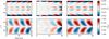Fig. 1 Test case KC1: comparison of the updated Leighton model with the results of the 2D dynamo run presented in Fig. 9 of Karak & Cameron (2016). The left column gives the results of the 2D run, showing time-latitude diagrams for the radial field at the surface (upper panel) and the radially averaged toroidal field (lower panel). The other two columns show the results of the updated Leighton model: using parameters corresponding to those of the 2D model (middle column) and with the diffusivity in the convection zone increased so that the dynamo has zero linear growth rate (right column). The quantities are normalized by a common factor, such that the extrema of ⟨ Bφ ⟩ become ±1.

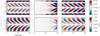Fig. 2 Test case KC2: same as Fig. 1, but for the 2D dynamo run shown in Fig. 11 of Karak & Cameron (2016).

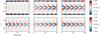Fig. 3 Test case J: same as Fig. 1, but for a 2D dynamo run carried out with the code used by Jiang et al. (2013). In this case, the lower row gives the (normalized) radially integrated toroidal flux.

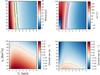Fig. 4 Properties of linear dynamo solutions as functions of the amplitude of the effective return meridional flow (V0) and of the magnetic diffusivity in the convection zone (η0) for values of α = 1.4 m s-1 and ϵ = 1. Color shading represents the dynamo period (P, upper left panel), the phase difference between the maximum of the polar field and the maximum rate of flux emergence (Δφ, upper right panel), and the dynamo growth rate (γ, lower left panel), all for dipole parity. The growth rate for quadrupolar parity is given in lower right panel. The lines in the lower panels indicate γ = 0, thus dividing regions of excited (reddish) and decaying (blueish) dynamo solutions. The lines in the upper panels indicate ranges relevant for the solar dynamo: 21 yr ≤ P ≤ 23 yr for the period and 80° ≤ Δφ ≤ 100° for the phase difference.

In all cases, the results of the 2D runs and those from our updated L69 model are very similar: dynamo periods, the shape of the butterfly diagrams, and the phase relation between the polar fields and the low-latitude toroidal field (representing flux emergence and solar activity) are reasonably well represented by our much simpler L69 model. There are some minor differences; for example, the periods are slightly longer and the low-latitude surface fields somewhat stronger relative to the polar fields in the L69 cases, but a perfect agreement is obviously not expected. We thus conclude that the updated L69 model captures the essential features of these moderately diffusive 2D models.

4. Parameter study

The computational efficiency of the updated L69 model allows us to systematically cover wide ranges of the parameter values relevant for the dynamo behavior. Since many of these parameters (e.g., meridional flow pattern and magnetic diffusivity in the convection zone, amplitude of the source term) are uncertain, this is a great advantage in comparison to the numerically more demanding 2D models. We have thus carried out a parameter study in order to identify those regions of the parameter space providing dynamo models that are consistent with basic properties of the solar cycle. To this end we require a) preference of the (antisymmetric) dipole mode; b) equatorward propagation of the activity belts; c) cycle period P ≃ 22 yr; and d) phase difference between the maxima of flux emergence (solar activity) and polar field Δφ ≃ 90°, meaning that the polar fields reverse around activity maxima and reach their peak levels around activity minima. The dynamo also must be excited (i.e., growth rate γ> 0).

A first representation of the results is given in Fig. 4. For fixed values of α = 1.4 m s^-1 and ϵ = 1, the upper panels give period, P, and phase difference, Δφ, for dipole parity. The lower panels show the dynamo growth rate, γ, for the dipole mode (left) and for the quadrupole mode (right). The lines in the upper panels indicate ranges relevant for the solar case. The lines in the lower panels separates regions of excited (lower) and non-excited (upper) dynamo solutions. The figure shows that the updated L69 model has a clear preference for dipolar parity in the sense that it is excited in a broader range of diffusivities (i.e., for lower dynamo number) and that its growth rate is always higher than that of the corresponding quadrupole mode. Furthermore, the results are consistent with the period and phase difference in the case of the Sun for diffusivities below about 80 km²s^-1 and an effective return flow of the meridional circulation affecting the toroidal field in the range 2–3 m s^-1.

An example of a solution with solar-like properties is shown in Fig. 5. It has a period of 20.3 yr and the correct phase difference between polar field and flux emergence (Δφ = 92°). Since the amplitude of this linear dynamo model is arbitrary, we fixed the maxima of the surface field, B_r, to 1 G. The corresponding values of the integrated toroidal flux, F_φ, are consistent with the expected amount of flux residing in the solar convection zone. This flux is mainly located in latitudes below 45°, which means that, in agreement with observation, flux emergence is also largely restricted to low latitudes. This behavior results mainly from the fact that B_φ is generated by the latitudinal rotational shear, which has its highest values in mid latitudes, together with the equatorward flux transport by the meridional return flow. Flux-transport dynamos relying on radial differential rotation near the bottom of the convection zone, on the other hand, face the problem that the generation of the toroidal flux mainly takes place in high latitudes (e.g. Nandy & Choudhuri 2002).

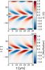Fig. 5 Example of a solar-like dynamo solution for the parameter values η0 = 80 km2s-1, α = 1.4 m s-1, ϵ = 1, V0 = 2.5 m s-1. Shown are time-latitude diagrams of the radial field at the surface (normalized to a maximum value of 1 G, upper panel) and of the radially integrated toroidal magnetic flux (per radian, lower panel).

The full results of our parameter study are summarized in Fig. 6. Here we show only the results for dipole parity because it is invariably the preferred mode. The four parameters describing the subsurface dynamics that we consider are the source amplitude, α, the diffusivity, η₀, the effective return flow amplitude, V₀, and the quantity 0 ≤ ϵ ≤ 1, which represents radial differential rotation below the near-surface shear layer. We represent the results in a similar form to those in Fig. 4 with panels indicating phase difference, period, and dynamo excitation as functions of V₀ and η₀. We now give a number of such panels for various values of α and ϵ which are indicated by the black bars at the bottom and at the left side of the figure. The individual panels represent the dynamo growth rate (positive in the orange shaded regions) and indicate relevant solar ranges for the dynamo period (P between 21 and 23 yr, green bands) and the phase difference (Δφ between 80° and 100°, purple bands). For each panel, we have calculated 153 models (using 17 values for V₀ in the range 0–8 m s^-1 and 9 values for η₀ in the range 10–90 km²s^-1).

Figure 6 shows that the domain of excited dynamos (positive growth rate) grows for increasing values of ϵ, reflecting the contribution of the NSSL to dynamo excitation. The band of solar values for the phase difference between maximum polar field and maximum flux emergence (purple bands) is not strongly affected by changes in α, η₀, and ϵ; in the domain of excited dynamos, permitted values are in most cases reached for return flow amplitudes in the range 2–4 m s^-1. Similarly, the dynamo period lies in the solar regime for the same range of return flow velocities. For the highest values of α and not too low ϵ, periods around 22 yr are only reached for very slow return flow, indicating that the character of the dynamo in this regime (represented by the panels located in the upper right part of the figure) has changed from transport-dominated to a dynamo wave driven by the NSSL. However, in these cases, the phase difference does not match the required value around 90°, so they cannot be considered as possible models for the solar dynamo.

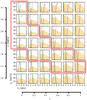Fig. 6 Results of the complete parameter study, for which all four parameters describing the subsurface dynamics were varied. For each set of parameters, a simulation was performed and the dynamo period, growth rate, and phase difference between the emergence rate and polar fields was determined. The green bands indicate the range of periods between 21 and 23 yr, the purple bands the range of the phase difference between 80° and 100°. The regions shaded in orange indicate dynamo excitation (positive growth rate). The red outline encloses those panels where solutions matching all three constraints exist.

The panels enclosed by the thick red contour in Fig. 6 show an overlap of the bands of solar values for period and phase difference. For lower values of ϵ (less effect of the NSSL), higher values of α are required to achieve solar-like behavior. In the overlap regions, the return flow amplitude typically has a speed of 2–3 m s^-1. Considering the sinusoidal profile of the return flow (∝sin2θ) with the extrema reached at ±45° latitude, this value is consistent with the observed latitudinal propagation of the activity belts of about 2° per year (corresponding to about 1 m s^-1). The overlap regions are typically located not far away from the line of marginal dynamo excitation (border of the orange region). Table 2 gives the parameter ranges for which the simulations match the solar values of the period, phase difference, and growth rate.

5. Discussion an conclusions

We have shown that the dynamo model of Leighton (1969) can be updated to include further relevant ingredients (meridional circulation, convective pumping, near-surface shear layer), so that the results are consistent with those of more involved 2D flux transport dynamo models. The uncertainties of the structure of magnetic field and flows in the convection zone can be condensed into a few free parameters while the computational simplicity of the model allows us to systematically scan the associated parameter space. Requiring some essential properties of the solutions (such as period, parity, phase relation between flux emergence and polar fields, positive linear growth rate) to agree with their observed solar counterparts, we were able to strongly narrow down the parameter space relevant for the solar dynamo.

We find that the Sun most probably hosts a flux-transport dynamo (as opposed to a dynamo wave driven by the NSSL) operating not too far from the threshold of marginal excitation. This property is consistent with recent results for other active stars (van Saders et al. 2016; Metcalfe et al. 2016). The effective equatorward return flow amplitude for the toroidal flux should be around 2 m s^-1, which is consistent with the latitudinal drift rate of the activity belts. Solar properties are achieved for values of the effective magnetic diffusivity for the toroidal flux as high as 80 km²s^-1, which puts the dynamo in the class of “high-diffusivity dynamos” (e.g. Choudhuri 2015). High diffusivity is also indicated by the observed properties of the solar activity belts (Cameron & Schüssler 2016).

The assumption that the tachocline shear is mostly irrelevant for the generation of toroidal magnetic flux (Spruit 2011; Cameron & Schüssler 2015; Wright & Drake 2016) leads to toroidal field and flux emergence concentrated in low latitudes (as observed) in a natural way: the rotational shear due to latitudinal differential rotation peaks at mid latitudes and the deep meridional return flow transports the toroidal flux equatorward.

As developed here, our updated L69 model is still linear. In reality, the cycle amplitudes are limited by a nonlinear back-reaction of the magnetic field on its sources. There are various possibilities for such a nonlinearity. While significant suppression of the rotational shear seems unlikely given the small variations of solar rotation during the activity cycle (Howe 2009), the most promising candidate appears to be a back-reaction on the active-region tilt angle, which is central ingredient of the poloidal field source. Dasi-Espuig et al. (2010) and McClintock & Norton (2013) indeed found indications for such an effect by analysing historical sunspot data (see, however Wang et al. 2015). Possibilities for the physical mechanism are enhanced resistance of stronger fields against the Coriolis force (before emergence), thermal effects near the base of the convection zone (Işık 2015), or the effect of active-region horizontal inflows (Cameron & Schüssler 2012; Martin-Belda & Cameron 2016). Nonlinear effects could modify the parameter space identified here for the operation of the solar dynamo. However, given that the dynamo probably operates near the excitation threshold, we do not expect very strong nonlinear effects.

In addition to scanning a large parameter space, the simplicity and computational efficiency of the quasi-1D L69 model also allow us to perform computations covering thousands of cycles. In a forthcoming paper, we will exploit this property to study how random variations of the source term affect the variability of the solar cycle over long time scales.

References

Appendix A: A violation of the Parker-Yoshimura rule?

The first case discussed in the results section of Leighton (1969, henceforth L69) involves a model with purely latitudinal differential rotation. It shows oscillatory solutions with latitudinally propagating dynamo waves, leading to solar-like butterfly diagrams of the toroidal and radial field components (cf. Figs. 1 and 2 in L69). However, if Leighton’s model is indeed mathematically equivalent to the αΩ formalism as indicated by Stix (1974), then dynamo waves should always propagate along isorotation surfaces (Yoshimura 1975). Since this property can already be inferred from the Cartesian model of Parker (1955), it is commonly known as the Parker-Yoshimura rule. Consequently, a purely latitudinal gradient of the angular velocity should lead to radially propagating dynamo waves (see, e.g., Köhler 1973) and no latitudinal propagation, in striking contrast to Leighton’s result.

The origin of this apparent contradiction results from an error in Eq. (9) of L69, 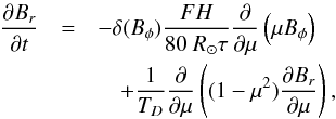$\begin{array}{ccc}\frac{\mathit{\partial }{\mathit{B}}_{\mathit{r}}}{\mathit{\partial t}}& \mathrm{=}& \mathrm{-}\mathit{\delta }\mathrm{\left(}{\mathit{B}}_{\mathit{\phi }}\mathrm{\right)}\frac{\mathit{FH}}{\mathrm{80}{\mathit{R}}_{\mathrm{\odot }}\mathit{\tau }}\frac{\mathit{\partial }}{\mathit{\partial \mu }}\mathrm{(}\mathit{\mu }{\mathit{B}}_{\mathit{\phi }}\mathrm{)}\\ & & \mathrm{+}\frac{\mathrm{1}}{{\mathit{T}}_{\mathit{D}}}\frac{\mathit{\partial }}{\mathit{\partial \mu }}\left(\mathrm{(}\mathrm{1}\mathrm{-}{\mathit{\mu }}^{\mathrm{2}}\mathrm{)}\frac{\mathit{\partial }{\mathit{B}}_{\mathit{r}}}{\mathit{\partial \mu }}\right)\mathit{,}\end{array}$(A.1)where μ = cosθ and F, H, T_D, and τ are parameters of the model. The critical quantity is the function δ(B_φ), which expresses the assumption that bipolar regions contributing to the regeneration of the poloidal field are only formed if the toroidal field exceeds a threshold value, B_c: 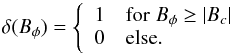$\mathit{\delta }\mathrm{\left(}{\mathit{B}}_{\mathit{\phi }}\mathrm{\right)}\mathrm{=}\{\begin{array}{c}\\ \mathrm{1}& \mathrm{for}{\mathit{B}}_{\mathit{\phi }}\mathrm{\ge }\mathrm{\left|}{\mathit{B}}_{\mathit{c}}\mathrm{\right|}\\ \mathrm{0}& \mathrm{else}\mathit{.}\end{array}$(A.2)Since B_φ depends on θ, this means that δ(B_φ) is an implicit function of θ. Consistent with the double-ring formalism of L69, this quantity must therefore be placed within the differentiation operator in the first term on the right-hand side of Eq. (A.1), so that this term, ℛ, should correctly read $\mathrm{ℛ}\mathrm{=}\frac{\mathit{FH}}{\mathrm{80}{\mathit{R}}_{\mathrm{\odot }}\mathit{\tau }}\frac{\mathit{\partial }}{\mathit{\partial \mu }}\mathrm{[}\mathit{\mu }\hspace{0.17em}\mathit{\delta }\mathrm{(}{\mathit{B}}_{\mathit{\phi }}\mathrm{\left)}{\mathit{B}}_{\mathit{\phi }}\mathrm{\right]}\mathit{.}$(A.3)

Only for constant δ (i.e., B_c = 0), as apparently also assumed by Stix (1974), is Leighton’s formulation correct (and consistent with the αΩ formalism). For B_c ≠ 0, the regeneration term as written in Eq. (A.1) leads to unphysical results. This can be most easily seen by considering the quantity 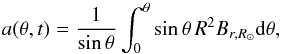$\mathit{a}\mathrm{\left(}\mathit{\theta ,t}\mathrm{\right)}\mathrm{=}\frac{\mathrm{1}}{\sin \mathit{\theta }}{\mathrm{\int }}_{\mathrm{0}}^{\mathit{\theta }}\sin \mathit{\theta }\hspace{0.17em}{\mathit{R}}^{\mathrm{2}}{\mathit{B}}_{\mathit{r,}{\mathit{R}}_{\mathrm{\odot }}}\mathrm{d}\mathit{\theta ,}$(A.4)which is proportional to the vector potential for B_r. Integrating Eq. (A.1), we obtain $\begin{array}{ccc}\frac{\mathit{\partial a}}{\mathit{\partial t}}& \mathrm{=}& \mathrm{-}\frac{\mathit{FH}{\mathit{R}}_{\mathrm{\odot }}\mathit{/}\mathrm{80}}{\mathit{\tau }\sin \mathit{\theta }}\left[\mathit{\delta }\mathrm{\left(}{\mathit{B}}_{\mathit{\phi }}\mathrm{\right)}{\mathit{B}}_{\mathit{\phi }}\cos \mathit{\theta }\mathrm{+}{\mathrm{\int }}_{\mathrm{0}}^{\mathit{\theta }}\frac{\mathit{\partial \delta }}{\mathit{\partial \theta }}{\mathit{B}}_{\mathit{\phi }}\cos \mathit{\theta }\hspace{0.17em}\mathrm{d}\mathit{\theta }\right]\\ & & \end{array}$(A.5)In the language of Yoshimura (1975), the first term on the right-hand side of Eq. (A.5) represents the “regeneration action” (see his Eq. (2.1)). In this case, the term contains a spatial derivative (i.e., it is not real in Yoshimura’s sense), so that his theorem does not apply and latitudinal migration is not excluded for purely latitudinal differential rotation.

Moreover, the incorrect term in Eq. (A.1) violates ∇·B = 0, which requires ∂(asinθ) /∂t = 0 for θ = π at all times, so that the radial flux integrated over the entire solar surface vanishes. This condition is trivially satisfied for the first term in the angular brackets on the right-hand side of Eq. (A.5) since B_φ = 0 at the poles, but the second term involving ∂δ/∂θ does not necessarily vanish for θ = π. In the case of the Heaviside function used by Leighton (see Eq. (A.2)) we have 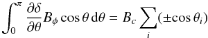${\mathrm{\int }}_{\mathrm{0}}^{\mathit{\pi }}\frac{\mathit{\partial \delta }}{\mathit{\partial \theta }}{\mathit{B}}_{\mathit{\phi }}\cos \mathit{\theta }\hspace{0.17em}\mathrm{d}\mathit{\theta }\mathrm{=}{\mathit{B}}_{\mathit{c}}\sum _{\mathit{i}}\mathrm{(}\mathrm{\pm }\cos {\mathit{\theta }}_{\mathit{i}}\mathrm{)}$(A.6)where the sum is over the points where | B_φ | = B_c and the sign depends on whether δ jumps from 0 to 1 or vice versa. Clearly, this sum in most cases does not vanish, so that ∇·B is not guaranteed. Numerical experiments show that the dynamo solutions with no radial shear reported in L69 decay when the correct form of Eq. (A.1), which maintains the divergence condition, is used.

All Tables

All Figures

Fig. 1 Test case KC1: comparison of the updated Leighton model with the results of the 2D dynamo run presented in Fig. 9 of Karak & Cameron (2016). The left column gives the results of the 2D run, showing time-latitude diagrams for the radial field at the surface (upper panel) and the radially averaged toroidal field (lower panel). The other two columns show the results of the updated Leighton model: using parameters corresponding to those of the 2D model (middle column) and with the diffusivity in the convection zone increased so that the dynamo has zero linear growth rate (right column). The quantities are normalized by a common factor, such that the extrema of ⟨ Bφ ⟩ become ±1.

In the text

	Fig. 2 Test case KC2: same as Fig. 1, but for the 2D dynamo run shown in Fig. 11 of Karak & Cameron (2016).
In the text

	Fig. 3 Test case J: same as Fig. 1, but for a 2D dynamo run carried out with the code used by Jiang et al. (2013). In this case, the lower row gives the (normalized) radially integrated toroidal flux.
In the text

Fig. 4 Properties of linear dynamo solutions as functions of the amplitude of the effective return meridional flow (V0) and of the magnetic diffusivity in the convection zone (η0) for values of α = 1.4 m s-1 and ϵ = 1. Color shading represents the dynamo period (P, upper left panel), the phase difference between the maximum of the polar field and the maximum rate of flux emergence (Δφ, upper right panel), and the dynamo growth rate (γ, lower left panel), all for dipole parity. The growth rate for quadrupolar parity is given in lower right panel. The lines in the lower panels indicate γ = 0, thus dividing regions of excited (reddish) and decaying (blueish) dynamo solutions. The lines in the upper panels indicate ranges relevant for the solar dynamo: 21 yr ≤ P ≤ 23 yr for the period and 80° ≤ Δφ ≤ 100° for the phase difference.

In the text

	Fig. 5 Example of a solar-like dynamo solution for the parameter values η0 = 80 km2s-1, α = 1.4 m s-1, ϵ = 1, V0 = 2.5 m s-1. Shown are time-latitude diagrams of the radial field at the surface (normalized to a maximum value of 1 G, upper panel) and of the radially integrated toroidal magnetic flux (per radian, lower panel).
In the text

Fig. 6 Results of the complete parameter study, for which all four parameters describing the subsurface dynamics were varied. For each set of parameters, a simulation was performed and the dynamo period, growth rate, and phase difference between the emergence rate and polar fields was determined. The green bands indicate the range of periods between 21 and 23 yr, the purple bands the range of the phase difference between 80° and 100°. The regions shaded in orange indicate dynamo excitation (positive growth rate). The red outline encloses those panels where solutions matching all three constraints exist.

In the text

References

- Babcock, H. W. 1961, ApJ, 133, 572 [Google Scholar]
- Barekat, A., Schou, J., & Gizon, L. 2014, A&A, 570, L12 [NASA ADS] [CrossRef] [EDP Sciences] [Google Scholar]
- Cameron, R. H., & Schüssler, M. 2007, ApJ, 659, 801 [NASA ADS] [CrossRef] [Google Scholar]
- Cameron, R. H., & Schüssler, M. 2012, A&A, 548, A57 [NASA ADS] [CrossRef] [EDP Sciences] [Google Scholar]
- Cameron, R. H., & Schüssler, M. 2015, Science, 347, 1333 [NASA ADS] [CrossRef] [Google Scholar]
- Cameron, R. H., & Schüssler, M. 2016, A&A, 591, A46 [NASA ADS] [CrossRef] [EDP Sciences] [Google Scholar]
- Cameron, R. H., Schmitt, D., Jiang, J., & Işık, E. 2012, A&A, 542, A127 [NASA ADS] [CrossRef] [EDP Sciences] [Google Scholar]
- Charbonneau, P. 2010, Liv. Rev. Sol. Phys., 7, 3 [Google Scholar]
- Choudhuri, A. R. 2015, J. Astrophys. Astron., 36, 5 [NASA ADS] [CrossRef] [Google Scholar]
- Choudhuri, A. R., Schussler, M., & Dikpati, M. 1995, A&A, 303, L29 [NASA ADS] [Google Scholar]
- Dasi-Espuig, M., Solanki, S. K., Krivova, N. A., Cameron, R., & Peñuela, T. 2010, A&A, 518, A7 [NASA ADS] [CrossRef] [EDP Sciences] [Google Scholar]
- Duvall, T. L., Dziembowski, W. A., Goode, P. R., et al. 1984, Nature, 310, 22 [NASA ADS] [CrossRef] [Google Scholar]
- Gizon, L., Birch, A. C., & Spruit, H. C. 2010, ARA&A, 48, 289 [Google Scholar]
- Hathaway, D. H., & Rightmire, L. 2011, ApJ, 729, 80 [Google Scholar]
- Hazra, S., & Nandy, D. 2016, ApJ, 832, 9 [NASA ADS] [CrossRef] [Google Scholar]
- Hazra, G., Karak, B. B., & Choudhuri, A. R. 2014, ApJ, 782, 93 [NASA ADS] [CrossRef] [Google Scholar]
- Howard, R. 1979, ApJ, 228, L45 [NASA ADS] [CrossRef] [Google Scholar]
- Howe, R. 2009, Liv. Rev. Sol. Phys., 6, 1 [Google Scholar]
- Işık, E. 2015, ApJ, 813, L13 [NASA ADS] [CrossRef] [Google Scholar]
- Jiang, J., Cameron, R. H., Schmitt, D., & Işık, E. 2013, A&A, 553, A128 [NASA ADS] [CrossRef] [EDP Sciences] [Google Scholar]
- Jiang, J., Hathaway, D. H., Cameron, R. H., et al. 2014, Space Sci. Rev., 186, 491 [Google Scholar]
- Jouve, L., Brun, A. S., Arlt, R., et al. 2008, A&A, 483, 949 [NASA ADS] [CrossRef] [EDP Sciences] [Google Scholar]
- Karak, B. B., & Cameron, R. H. 2016, ApJ, 832, 94 [NASA ADS] [CrossRef] [Google Scholar]
- Karak, B. B., Jiang, J., Miesch, M. S., Charbonneau, P., & Choudhuri, A. R. 2014, Space Sci. Rev., 186, 561 [NASA ADS] [CrossRef] [Google Scholar]
- Köhler, H. 1973, A&A, 25, 467 [NASA ADS] [Google Scholar]
- Komm, R. W., Howard, R. F., & Harvey, J. W. 1995, Sol. Phys., 158, 213 [NASA ADS] [Google Scholar]
- Krause, F., & Rädler, K. H. 1980, Mean-field magnetohydrodynamics and dynamo theory (Oxford: Pergamon Press) [Google Scholar]
- Leighton, R. B. 1964, ApJ, 140, 1547 [Google Scholar]
- Leighton, R. B. 1969, ApJ, 156, 1 [Google Scholar]
- Lemerle, A., Charbonneau, P., & Carignan-Dugas, A. 2015, ApJ, 810, 78 [NASA ADS] [CrossRef] [Google Scholar]
- Mackay, D., & Yeates, A. 2012, Liv. Rev. Sol. Phys., 9, 6 [Google Scholar]
- Martin-Belda, D., & Cameron, R. H. 2016, A&A, 586, A73 [NASA ADS] [CrossRef] [EDP Sciences] [Google Scholar]
- McClintock, B. H., & Norton, A. A. 2013, Sol. Phys., 287, 215 [NASA ADS] [CrossRef] [Google Scholar]
- Metcalfe, T. S., Egeland, R., & van Saders, J. 2016, ApJ, 826, L2 [Google Scholar]
- Miesch, M. S., & Teweldebirhan, K. 2016, Adv. Space Res., 58, 1571 [NASA ADS] [CrossRef] [Google Scholar]
- Muñoz-Jaramillo, A., Dasi-Espuig, M., Balmaceda, L. A., & DeLuca, E. E. 2013, ApJ, 767, L25 [Google Scholar]
- Nandy, D., & Choudhuri, A. R. 2002, Science, 296, 1671 [NASA ADS] [CrossRef] [PubMed] [Google Scholar]
- Ossendrijver, M., Stix, M., Brandenburg, A., & Rüdiger, G. 2002, A&A, 394, 735 [NASA ADS] [CrossRef] [EDP Sciences] [Google Scholar]
- Parker, E. N. 1955, ApJ, 122, 293 [NASA ADS] [CrossRef] [Google Scholar]
- Parker, E. N. 1984, ApJ, 281, 839 [NASA ADS] [CrossRef] [Google Scholar]
- Route, M. 2016, ApJ, 830, L27 [NASA ADS] [CrossRef] [Google Scholar]
- Schou, J., Antia, H. M., Basu, S., et al. 1998, ApJ, 505, 390 [NASA ADS] [CrossRef] [Google Scholar]
- Spruit, H. C. 2011, in The Sun, the Solar Wind, and the Heliosphere, eds. M. P. Miralles, & J. Sánchez Almeida, 39 [Google Scholar]
- Stix, M. 1974, A&A, 37, 121 [Google Scholar]
- Thompson, M. J., Toomre, J., Anderson, E. R., et al. 1996, Science, 272, 1300 [NASA ADS] [CrossRef] [PubMed] [Google Scholar]
- Usoskin, I. G. 2013, Liv. Rev. Sol. Phys., 10, 1 [Google Scholar]
- van Saders, J. L., Ceillier, T., Metcalfe, T. S., et al. 2016, Nature, 529, 181 [NASA ADS] [CrossRef] [PubMed] [Google Scholar]
- Vasil, G. M., & Brummell, N. H. 2009, ApJ, 690, 783 [NASA ADS] [CrossRef] [Google Scholar]
- Wang, Y.-M. 2016, Space Sci. Rev., DOI: 10.1007/s11214-016-0257-0 [Google Scholar]
- Wang, Y.-M., & Sheeley, Jr., N. R. 1991, ApJ, 375, 761 [NASA ADS] [CrossRef] [Google Scholar]
- Wang, Y.-M., & Sheeley, N. R. 2009, ApJ, 694, L11 [NASA ADS] [CrossRef] [Google Scholar]
- Wang, Y.-M., Sheeley, Jr., N. R., & Nash, A. G. 1991, ApJ, 383, 431 [NASA ADS] [CrossRef] [Google Scholar]
- Wang, Y.-M., Colaninno, R. C., Baranyi, T., & Li, J. 2015, ApJ, 798, 50 [NASA ADS] [CrossRef] [Google Scholar]
- Wright, N. J., & Drake, J. J. 2016, Nature, 535, 526 [NASA ADS] [CrossRef] [PubMed] [Google Scholar]
- Yoshimura, H. 1975, ApJ, 201, 740 [NASA ADS] [CrossRef] [Google Scholar]