| Issue |
A&A
Volume 599, March 2017
|
|
|---|---|---|
| Article Number | A102 | |
| Number of page(s) | 8 | |
| Section | Interstellar and circumstellar matter | |
| DOI | https://doi.org/10.1051/0004-6361/201629721 | |
| Published online | 09 March 2017 | |
Testing dust trapping in the circumbinary disk around GG Tauri A
1 Max-Planck-Institut für Extraterrestrische Physik, Gieβenbachstraβe, 85741 Garching bei München, Germany
e-mail: pcazzoletti@mpe.mpg.de
2 Harvard-Smithsonan Center for Astrophysics, 60 Garden Street MS68, Cambridge, MA 02138, USA
3 Universitá degli Studi di Milano, via Giovanni Celoria 16, 20133 Milano, Italy
4 Max-Planck-Institut für Astronomie, Königstuhl 17, 69117 Heidelberg, Germany
Received: 14 September 2016
Accepted: 26 October 2016
Context. The protoplanetary disk around the GG Tau A binary system is one of the most studied young circumbinary disk, and it has been observed at many different wavelengths. Observations of the dust continuum emission at sub-mm/mm wavelengths have detected a dust ring located between 200 AU and 300 AU from the center of mass of the system. According to the classical theory of tidal interaction between a binary system and its circumbinary disk, the measured inner radius of the mm-sized dust ring is significantly larger than the predicted truncation radius, given the observed projected separation of the stars in the binary system (0.25′′, corresponding to ~ 34 AU). A possible explanation for this apparent tension between observations and theory is that a local maximum in the gas radial pressure is created at the location of the center of the dust ring in the disk as a result of the tidal interaction with the binary. An alternative scenario invokes the presence of a misalignment between the disk and the stellar orbital planes.
Aims. We investigate the origin of this dust ring structure in the GG Tau A circumbinary disk, test whether the interaction between the binary and the disk can produce a gas pressure radial bump at the location of the observed ring, and discuss whether the alternative hypothesis of a misaligned disk offers a more viable solution.
Methods. We run a set of 3D hydrodynamical simulations for an orbit consistent with the astrometric solutions for the GG Tau A stellar proper motions, different disk temperature profiles, and for different levels of viscosity. Using the obtained gas surface density and radial velocity profiles, we then apply a dust evolution model in post-processing in order to to retrieve the expected distribution of mm-sized grains.
Results. We compare the results of our models with the observational results and show that, if the binary orbit and the disk were coplanar, not only would the tidal truncation of the circumbinary disk occur at a radius that is too small with respect to the inner edge inferred by the dust observations – which is in agreement with classical theory of tidal truncation − but also that the pressure bump and the dust ring in the models would be located at <150 AU from the center of mass of the stellar system. This shows that the GG Tau A circumbinary disk cannot be coplanar with the orbital plane of the binary. We also discuss the viability of the misaligned disk scenario, suggesting that in order for dust trapping to occur at the observed radius, the disk and orbital plane must be misaligned by an angle of about 25−30 degrees.
Key words: protoplanetary disks / hydrodynamics / accretion, accretion disks / binaries: close / planets and satellites: rings
© ESO, 2017
1. Introduction
Most stars form in multiple systems (e.g. Duquennoy & Mayor 1991; Fischer & Marcy 1992; Raghavan et al. 2010). It is also undisputed that the majority of stars in young star forming regions show direct or indirect evidence of the presence of a young circumstellar disk. Moreover, disks orbiting the whole multiple stellar system, called circumbinary in the case of binary systems, are sometimes observed (e.g. Simon & Prato 1995). Planets originate from these disks, and so far ten circumbinary planets (sometimes called “Tatooine planets”) have been discovered by Kepler orbiting around eight eclipsing binaries (Doyle et al. 2011; Welsh et al. 2012; Orosz et al. 2012a,b; Schwamb et al. 2013; Kostov et al. 2013, 2014; Welsh et al. 2014). Planets, therefore, are common in binary (or multiple) systems.
Disk-binary interaction plays a pivotal role in such systems. In binaries, part of the material of a disk around one or both stars is ripped away by tidal forces. The net result of the interaction between the gas disk and the binary is a net exchange of angular momentum via tidal torques. In particular, the angular momentum of the disk-binary system is transported outwards (Lin & Papaloizou 1979a,b). This means that gas in the individual circumstellar disks loses angular momentum to the binary and moves toward inner orbits; the gas in circumbinary disks, on the other hand, acquires angular momentum from the binary and is repelled from the central stars. Disk viscosity tends to contrast the effect of tidal torques. At a certain radius, called the tidal truncation radius, viscous and tidal torques balance each other and an equilibrium configuration is reached (Lin & Papaloizou 1986).
Theoretical studies have attempted to find a model capable of providing an estimate of the radius of each one of the three disks in a binary system (i.e., circumprimary, circumsecondary, and circumbinary), given the key orbital parameters (semi-major axis a, eccentricity e, mass ratio q, and inclination i between disk and orbital plane) and some characterization of the disk viscosity (Papaloizou & Pringle 1977; Paczynski 1977; Artymowicz & Lubow 1994; Pichardo et al. 2005; Miranda & Lai 2015; Lubow et al. 2015). In one of the most comprehensive works so far Artymowicz & Lubow (1994) estimated the truncation radius for binaries coplanar with the disks and for any value of q, e and viscosity. Miranda & Lai (2015) recently generalized this study for misaligned systems.
Observations of young disks in multiple systems have the potential to test the predictions of tidal truncation theory (Harris et al. 2012). The best cases are offered by the systems in which the proper motion for the stellar components are measured for a significant fraction of the stellar orbits. In this case, orbital solutions are obtained from the analysis of the proper motions, and models incorporating the tidal interaction between the multiple system and the disks can be used to predict the spatial distribution of gas and dust in the disks. High angular resolution observations of the disk emission can then be used to test the predictions of the models. In this work we use the results of recent observations for the GG Tau A circumbinary disk to test models of tidal truncation.
The young quadruple system GG Tau has been the subject of many different studies. It is composed of two low-mass binary systems, namely GG Tau A and GG Tau B. GG Tau Aa and GG Tau Ab, respectively of mass 0.78 ± 0.09 M⊙ and 0.68 ± 0.02 M⊙ (White et al. 1999) and with an angular separation of 0.25′′ (Leinert et al. 1993), are the two components of GG Tau A, one of the most studied and best known nearby (~ 140 pc, Elias 1978) young binary systems (~ 1 Myr, White & Ghez 2001)1. Its circumbinary disk has been observed in dust thermal emission (Dutrey et al. 1994; Guilloteau et al. 1999; Andrews et al. 2014), in scattered light emission (Roddier et al. 1996; Silber et al. 2000; Duchêne et al. 2004), and in CO gas emission (Dutrey et al. 2014), and has a total mass of ~ 0.12 M⊙ and an inclination i = 37° with respect to the line of sight (Guilloteau et al. 1999) . The other binary system, GG Tau B, is located 10.1′′ south, is wider (1.48′′), and is less massive (Leinert et al. 1993).
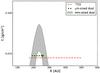 |
Fig. 1 Observational constraints available to date for different sized grains and for CO distribution. The gray-shaded area shows the 2σ uncertainty on the mm-sized dust radial density profile as modeled in Andrews et al. (2014). The red dash-dotted and the green dashed lines show the radial extent of CO and micron-sized dust grains, respectively. It should be noted that these two tracers are optically thick and do not provide information about the density profile. The vertical location of the lines is therefore arbitrary. |
Parameters of the best orbital solutions.
The disk around GG Tau A shows a peculiar ring-shaped dust distribution. Andrews et al. (2014) modeled the continuum dust emission measured at several millimeter wavelengths with a radial distribution for mm-sized grains as a Gaussian peaked at 235 ± 5 AU, and with a very narrow width, FWHM ~ 60 AU. Imaging in scattered light at near infrared wavelengths have shown that the inner radius of the disk in smaller, so that μm-sized particles lie between 180 and 190 AU (Duchêne et al. 2004). ALMA observations of the rotational transition J = 3−2 of 13CO show an intensity radial profile with a peak around 175−180 AU from the binary center (Tang et al. 2016). However the relatively poor spatial resolution of these observations (≈ 50 AU) does not allow the location of the inner radius in gas to be inferred with precision. Emission from both 12CO(J = 3−2) and 13CO(J = 3−2) is detected up to ~ 500 AU from the binary, clearly indicating that gas is also found at much larger radii than the mm-sized dust. Among all the components observed, only mm-sized dust grains are optically thin and can therefore provide information on the density profile of mm dust. For this reason, we will mainly focus our study on the dust ring observed at submillimeter wavelengths. A summary of the various constraints for the disk size in the various components is shown in Fig. 1.
In order to use this information on the spatial extent of the GG Tau A circumbinary disk to test the predictions of tidal truncation models, some constraints on the orbital parameters of the GG Tau A binary system are needed. For example, the classical calculations by Artymowicz & Lubow (1994) predict disk truncation radii at 2 or 3 times the value of the binary semi-major axis a. A number of astrometric observations for the GG Tau A system are available, and span almost twenty years from 1990 to 2009. However, these measurements cover only a fraction of the orbital period of the binary and do not allow all the orbital parameters to be constrained at the same time. By fixing one of the orbital parameters, all the others can be obtained by fitting the proper motions (Köhler 2011). Table 1 shows four different orbits consistent with the astrometric measurements: the first column is obtained by requiring that the disk and the binary orbit be coplanar (i.e., putting constraints on the inclination i of the orbit and on the position angle of its ascending node), while the other three are calculated by fixing the value of the semi-major axis of the orbit to 60,70, and 80 AU.
If the inclination i and the position angle of the ascending node of the binary orbit are constrained by requiring the orbit to be coplanar with the disk, then a ≈ 34 AU. In this case the dust inner ring is located much farther out than the predicted ~ 100 AU gas inner truncation radius. A possible explanation for this apparent discrepancy was proposed by Andrews et al. (2014): if the gas radial density profile at the inner edge of the disk were very shallow, then the pressure maximum where mm-size grains drift toward and accumulate would lie at a much larger radial position than the gaseous disk inner radius. Hydrodynamical simulations calculating the expected gas radial profile are needed to test this hypothesis.
Alternatively, if the hypothesis of coplanarity is relaxed, the astrometric measurements can be fit by orbits misaligned with respect to the disk plane and with higher values of a (as shown in Table 1). These misaligned configurations would allow the binary system to dynamically truncate the disk at a location closer to the observed dust ring. In this misaligned case, a steeper radial profile for the gas density would in principle also be able to produce a dust ring at radii even larger than 200 AU.
It should be noted that a coplanar disk-binary system with a> 34 AU is not entirely ruled out by the astrometric measurements, and that a coplanar orbit with a larger semi-major axis is still possible within a 5σ uncertainty. Owing to the much lower likelihood of this solution, however, we decide not to address it in this work. More astrometric measurements are needed for a more detailed analysis.
In this paper we run a set of hydrodynamical simulations that account for tidal interaction between the binary and the circumbinary disk to calculate the predicted distribution of gas density in the best-fit case of coplanar disk and binary system. We couple a dust evolution model (Birnstiel et al. 2010) to the results of the hydrodynamical simulations for the gas to obtain predictions for the radial profile of the dust density. We compare these predictions with the main features observed for the dust in the disk in order to test the validity of the coplanar hypothesis. We also discuss whether the alternative hypothesis of a misaligned disk could be a likely explanation for the location of the dust observed in the GG Tau A circumbinary disk. For this study, we always consider orbital parameters that are consistent with the measured stellar proper motions.
In Sect. 2 we briefly present the setup of our simulations. In Sects. 3 and 4 we show the results we obtained in our simulations and we discuss the effect that our results have on the search for an explanation for the observed narrow mm-dust ring.
2. Methods
2.1. Gas simulations
In our work we use the PHANTOM Smoothed Particle Hydrodynamics (SPH) code (Lodato & Price 2010; Price & Federrath 2010) in order to perform 3D hydrodynamical simulations for the gas alone. The code computes the viscous evolution of a gas distribution in a disk by solving the equations of hydrodynamics in the presence of a gravitational field generated by one or two central stars and/or a planetary mass companion. For our purposes, we use a circumbinary disk and we neglect its self-gravity. We want to study the resulting gas radial density and velocity profiles.
To mimic disk viscosity, we adopt the formulation by Flebbe et al. (1994), where the stress tensor in evaluated directly in the Navier-Stokes equations.We can express the shear viscosity using the Shakura & Sunyaev (1973) prescription  (1)where α is the chosen value for the Shakura & Sunyaev (1973) parameter, and cs(R) and Ω(R) are the sound-speed and angular velocity radial profiles, respectively. The accuracy of this formulation has also been tested for physical phenomena strongly dependent on the chosen value of α, such as the dynamics of warps (Lodato & Price 2010; Facchini et al. 2013).
Since the disk viscosity strongly affects both the location of the tidal truncation radius and the dust dynamics, we choose to run a set of different simulations using three different values of viscosity, corresponding to α of 0.01, 0.005 and 0.002.
A second source of viscosity is also present. SPH codes implement an artificial viscosity in order to be able to resolve discontinuities by spreading them over a few smoothing lengths and to prevent particle interpenetration. This artificial term can be understood as a numerical representation of second derivatives of the velocity (Artymowicz & Lubow 1994; Murray 1996; Lodato & Price 2010); the resulting artificial viscosity parameter is given by  (2)where ⟨h⟩ is the azimuthally averaged smoothing length (which is proportional to n− 1/3, n being the local density of SPH particles), H is the disk thickness, and αAV is set to a minumum value
  and increases up to a value
  in the presence of shocks by means of a Morris & Monaghan (1997) switch. We also note that we used the notation αart to discriminate between the physical viscosity due to the artificial term and the directly implemented physical viscosity, for which we used α. The total viscosity in SPH is therefore given by αtot ≈ α + αart.
Since ⟨h⟩ ∝ n− 1/3, we can make the contribution of the artificial viscosity to the physical viscosity negligible by increasing the number of particles in the low-viscosity simulations (see Sect. 2.3), thus making αtot ~ α.
In the simulations presented in this work, we set  and
and  . The Von Neumann & Richtmyer (1950)βAV parameter was set equal to 2. We let each simulation evolve over 1000 binary orbital periods in order to reach steady state. We then compute the gas density and the gas radial velocity profile by averaging the quantities azimuthally. We also average them over a few orbital periods in order to smooth the profiles and to remove the fluctuations due to the discretization of the fluid operated by SPH.
2.2. Dust simulations
We use the gas density and radial velocity profiles obtained from our SPH simulations as a stationary “environment” where we let the dust evolve following the model from Birnstiel et al. (2010). We assume that the gas density in a binary system reaches a stationary state on timescales shorter than the dust evolution timescales, which for typical dust-to-gas ratios are on the order of hundreds of local orbits (e.g., Brauer et al. 2008), which at the position of the dust ring is long compared to the binary orbital timescale (~ 200 yr). We use this stationary gas density distribution as input for a global model of dust evolution (Birnstiel et al. 2010) to test how dust evolves under the physical conditions predicted by the SPH hydrodynamical simulations.
Our dust evolution model accounts for compact dust growth, cratering and fragmentation, radial drift, turbulent mixing, and gas drag. In order to calculate the relative velocity of the dust particles, Brownian motion, turbulence, vertical settling, and radial and azimuthal drift are taken into account. In these simulations, the initial size of all the particles is assumed to be ~ 1 μm. At the beginning of the growth process, when particles have still sizes of a few microns, the main contribution to their relative velocities comes from Brownian motion and settling. In these early stages, growth by coagulation is very efficient and is a result of van der Waal’s interaction between small grains. As they grow to larger sizes, they start to decouple from the gas, and turbulence as well as radial drift become the main sources of their relative velocities.
As the grains grow, their relative velocities increase (Birnstiel et al. 2010). When dust grains reach sizes with high enough velocities, collisions no longer produce coagulation only, but can also cause the dust grains to fragment. The threshold velocities above which fragmentation becomes dominant can be estimated through laboratory experiments and theoretical work of collisions for silicates and ices (e.g. Blum & Wurm 2008; Schäfer et al. 2007; Wada et al. 2009). For the silica particles these threshold velocities are on the order of a m/s, and they increase with the presence of ices (Gundlach & Blum 2015). We ran some test models with different values of fragmentation velocity vfrag and we found that the results were not significantly affected. In our models we adopted a standard value of vfrag = 10 m/s.
The level of coupling between the dust and the gas is quantified with the dimensionless stopping time τfric, defined as the ratio between the stopping time of the particle due to friction with the gas and the orbital timescale Ω. Particles with τfric ≫ 1 are decoupled from the gas; they are not affected by any drag force and therefore rotate around the star on their own Keplerian orbit. On the other hand, particles with τfric ≪ 1 are strongly coupled with the gas and move along with it. Particles experiencing the biggest radial drift are those characterized by τfric = 1. In the case of the GG Tau A disk, in the vicinity of the observed dust ring we expect this to occur for grains with sizes of ~ 1−10 mm. Owing to the sub-Keplerian rotation velocity of the gas, these particles experience a gas headwind that leads them to lose angular momentum and to drift radially towards the disk inner regions (Whipple 1972; Nakagawa et al. 1986; Brauer et al. 2007).
One of the biggest unknowns for dust evolution models is whether dust growth is compact or fractal. In our models we assume compact growth. However, fractal and compact growth models are not expected to produce significantly different results in terms of the sub-mm emission from the disk outer regions because these different modes of solid growth produce particles with similar τfric (even though they have different sizes and filling factors) and absorption/emission dust opacities are proportional to τfric. Therefore, we do not expect this intrinsic uncertainty of the models to play an important role on the results of the work presented here.
In Sect. 3.3 we apply this dust model to simulate the behavior of dust particles in the coplanar case for the GG Tau A circumbinary disk. We use these results to compare the predictions of our models to the radial distribution of dust particles as constrained by the observations.
2.3. Initial conditions
We tune our initial conditions to reproduce the main characteristics of the GG Tau A system. First of all, the eccentricity e and the semi-major axis a of the orbit are set according to the best-fit orbits calculated by Köhler (2011) to reproduce the measured stellar proper motions (Table 1). In this work we are interested in simulating in detail the case of coplanar disk and binary orbital plane (second column in Table 1), but we also discuss the hypothesis of a disk misaligned with the binary which allows for higher values of the semi-major axis than in the coplanar case (a few possible cases are listed in Cols. 3−5 in Table 1).
In the SPH simulations, the two stars are modeled as sink particles (Bate et al. 1995) with mass 0.78 M⊙ and 0.68 M⊙ (White et al. 1999). Each of the two sink particles has an associated accretion radius, i.e. a radius within which we can consider gas particles to be accreted onto the stars. Since for our purposes we do not need to know what happens to the gas in the vicinity of the stars, we can set the sink radii to fairly high values, thus speeding up the simulations. In particular, we use Rsink = 0.1 a.
We set the initial disk inner and outer radii at t = 0 to Rin = 2a and Rout = 800 AU, respectively. Between these two edges, the initial gas density profile we use is  (3)where Σ0 is a normalization factor. Its value is chosen in each simulations in order to give a total gas mass of around ~ 0.12 M⊙ (the disk mass estimated by Guilloteau et al. 1999). We then set a Keplerian velocity profile for the gas, relative to a 1.46 M⊙ central mass. It should be noted that our hydrodynamical results do not depend on the initial gas density profile since we let our system evolve until steady state is reached. We assume for the gas a locally isothermal equation of state, where the temperature along the z-axis at each radius is fixed. To describe the temperature radial profile we adopted the one inferred from the analysis of 13CO measurements:
  (4)In order to test the effect of this choice for the disk temperature on the results of our study, we also ran simulations with a less steep temperature radial profile (T ∝ R-0.5; see Appendix A).
The temperature profile is related to the disk thickness H by assuming vertical hydrostatic equilibrium  (5)where μ = 2.3 is the mean molecular weight and kB is the Boltzmann constant. The particles are then distributed in the vertical direction to obtain a Gaussian density profile with thickness H(R). Combining Eqs. (4) and (5) we get H/R ≈ 0.12 in our simulations.
Among all the factors that affect the evolution of gas and dust in the disk, viscosity plays an important role. For this reason we decided to run different simulations for different values of viscosity. When simulating disks with lower viscosities, we correspondingly increased the number of SPH particles to reduce the possible effects given by the artificial viscosity, as explained in Sect. 2.1. In particular, we ran simulations with α = 0.01 (using 106 particles), α = 0.005 (using 3 × 10⁶ particles), and α = 0.002 (6 × 10⁶ particles). We obtain αart ≤ 0.002 in the 106 particles simulation, αart ≤ 0.0015 in the 3 × 10⁶ one, and αart ≤ 0.001 when using 6 × 10⁶ particles.
3. Results
In this section we present the results obtained with our simulations with a binary orbiting on the same plane of the disk. In this case, the binary orbit has a = 34 AU and e = 0.28. We study how the initial gas density profile evolves with time, and how it is affected by the chosen values of viscosity. Particular focus is given to how time and viscosity affect the location and shape of the gas density maximum because marginally coupled dust particles will radially drift to this region. In these simulations, the binary orbit has semi-major axis and eccentricity of a = 34 AU and e = 0.28, respectively, corresponding to the best-fit orbit solutions of the measured stellar proper motions (Col. 2 in Table 1).
3.1. Time evolution of the gas density profile
We first verify that the evolution time in our simulations (1000 orbital periods) is sufficient for the gas density profile to reach a steady state configuration. Figure 2 shows a comparison of the gas density profile at different times for the α = 0.002 simulation, i.e. the one with the longest viscous timescale. Even for the lowest viscosity, the density profiles after 750 and 1000 orbital periods differ by at most ~ 3%. We therefore assume that the disk has reached steady state after 1000 orbital periods.
3.2. Different viscosities
It is also important to test how the gas density profile is affected by different choices for the disk viscosity. Figure 3 shows the three gas density profiles (azimuthally and temporally averaged over a few binary orbital periods in order to remove numerical noise) corresponding to the three values of viscosity tested in our simulations. These profiles are compared to the density profile modeled in Andrews et al. (2014), which was proposed to reproduce the necessary dust trapping at the location where the dust ring of ~mm-sized grains was observed.
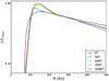 |
Fig. 2 Azimuthally averaged gas density profile for the α = 0.002 simulation at different evolutionary stages. After a few hundred binary orbits the density profile reaches a quasi-stationary configuration. All the density profiles are normalized to the maximum of the density profile at the end of the simulation. |
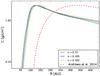 |
Fig. 3 Gas density profiles obtained from our simulations (solid lines) in the coplanar case using α = 0.01,0.005,0.002. The gas density profile invoked by Andrews et al. (2014) is also plotted (dashed line) for comparison. |
 |
Fig. 4 Snapshot of the inner cavity of the circumbinary disk at 1000 binary orbits in the α = 0.002 case. The white dots indicate the location of the two central stars; the dashed lines show the location of the pressure maximum. The image was produced using SPLASH (Price 2007). |
In all the three cases, our gas simulations produce very small tidal truncation radii (<100 AU), and a gas density peak located at radii of 130−140 AU, much smaller than in the profile proposed by Andrews et al. (2014). There is no strong dependence of the location of the gas density peak on the assumed value of α.
Figure 4 shows the inner cavity in a snapshot of our simulation α = 0.002 at 1000 binary orbits. The white dots mark the location of the two central stars, while the black dashed lines show the location of the maximum of the gas radial density profile.
3.3. Dust evolution
We use the dust evolution model from Birnstiel et al. (2010) to investigate the expected density distribution of dust in the disk. We apply these models to the outputs of the three coplanar case simulations, corresponding to the three values of viscosity.
We were able to obtain dust trapping for mm-sized grains only in the case of α = 0.002. For higher α values, mm-sized dust particles tend to fragment to smaller sizes (e.g. Birnstiel et al. 2012) and their trapping efficiency decreases (see Birnstiel et al. 2010) . As shown by the solid blue line in Fig. 5, at this low value of viscosity a large enough population of mm-sized grains is formed and it is efficiently trapped at ~ 150 AU, the location of the gas pressure maximum. However, the ring is too close to the central star and our results are inconsistent with the data, represented by the gray shaded area in Fig. 5.
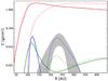 |
Fig. 5 Density profiles for gas (solid red line) and dust (solid blue for mm-sized and solid green for micron-sized) obtained from our simulations in the coplanar case using α = 0.002. The gas and dust density profiles from the model by Andrews et al. (2014) are also plotted (dashed lines) for comparison. It is clear that the solid blue line showing the mm-sized dust surface density profile is not consistent with the data (gray shaded area). |
This inconsistency cannot be solved by simply considering different values of viscosity or a different temperature profile. In fact, as shown in Sect. 3.2 and Appendix A, the gas density profile obtained from our hydrodynamical simulations does not depend strongly on these properties of the disk. Since the dust ring in mm-sized particles around GGTau A is due to dust trapping at the location of the gas pressure maximum, we can therefore conclude that the orbit of the binary and the disk cannot be coplanar: the large radial location of the ring cannot be explained by such a configuration since the gas density maximum, and consequently the dust ring, would lie at a radius that is too small compared to the position of the ring of mm-sized dust. The inner radius of micron sized grains is also strongly underestimated with respect to the 180−190 AU observed by Duchêne et al. (2004) and shown in Fig. 1.
4. Discussion
We tested the hypothesis that the narrow dust ring around GG Tau A can be explained by dust trapping at the gas density maximum. We showed that this scenario cannot be explained consistently with astrometric measurements by a binary orbiting on the same plane of the circumbinary disk. Indeed, the best-fit orbit calculated by Köhler (2011) without fixing any parameter gives a misalignment between the disk and the orbital plane of ~ 30° However, the uncertainties on the fitted orbital parameters in this case are much larger, given the poor sampling of the binary orbit.
If, on the one hand, the resulting separation between the two stars in this coplanar case is too small to explain the location of the dust ring, on the other hand, a binary orbit with a larger semi-major axis could in principle create such a wide ring. As a increases, the truncation radius for the gas component of the disk moves farther out, and the gas pressure bump trapping the dust is located at larger radii. The astrometric measurements for the proper motion of GG Tau A are consistent with wider binaries if the hypothesis of a disk coplanar with the binary motion is dropped and the binary and the disk are misaligned. Table 1 shows that orbits with a = 60−80 AU are consistent with misalignments between 25° and 30°. In the latter scenario, we expect the disk to become eccentric and warped, and our approach, which assumes azimuthal symmetry, would not be suitable to test it; instead 3D hydrodynamical simulations including gas and dust would be required (Laibe & Price 2014; Dipierro et al. 2015, 2016).
Tidal truncation itself is influenced by the misalignment between orbital and disk plane. Recently Lubow et al. (2015) studied the dependence of the tidal torque on the misalignment angle at the 2:1 inner Lindblad resonance in the case of a nearly circular disk rotating around a circular-orbit binary. Furthermore, Miranda & Lai (2015) quantitatively computed how the tidal truncation radius changes in misaligned systems with respect to coplanar ones, adopting a truncation criterion determined by the balance between resonant torque (which they analytically calculated for a misaligned system) and viscous torque. The latter study also took eccentric binaries into consideration. The common conclusion is that in general the torques in misaligned systems are weaker, and that circumbinary disks in such systems tend to have smaller inner radii than in the aligned case. Therefore, in principle, a wide range of truncation radii could be expected for circumbinary disks, and not only the classical 2−3a prediction from Artymowicz & Lubow (1994). In practice, Miranda & Lai (2015) show that this happens only for very misaligned systems (Δi ≳ 90°); in these cases, the inner radius of a circumbinary disk can decrease to 1−1.5a. We conclude that for a = 60−80 AU and for the relative binary-disk misalignment, we should expect tidal torques to truncate the disk between 180 and 240 AU.
Theoretical studies have shown that binaries and disks forming with different axes of rotation are not rare. For example, Bonnell et al. (1992) showed that in the case of an elongated cloud with a rotation axis is oriented arbitrarily with respect to the cloud axis, the disk plane (reflecting the angular momentum of the core) and the orbital plane (reflecting the symmetry of the initial core) can indeed be misaligned. Similarly, Bate et al. (2010) showed that during the star formation process, the variability of the angular momentum of the accreting material and dynamical interactions between stars can produce significant misalignment between the stellar rotation axis and the disk spin axis. However, tidal torques tend to realign the two planes. Foucart & Lai (2014) calculated this alignment torque, and concluded that we should expect circumbinary disks around close (sub-AU) binaries to be highly aligned, while disks and planets around wider binaries could still be misaligned. The latter is the case for GG Tau A, where we expect a ≈ 70 AU.
Some observations of misaligned circumbinary disks already exist. Imaging of circumbinary debris disks shows that the disk plane and the orbital plane are misaligned for some systems, such as 99 Herculis, where the mutual inclination is Δi ≳ 30° (Kennedy et al. 2012). Moreover, the pre-main sequence binary KH 15D is surrounded by a circumbinary disk inclined by 10°−20° with respect to the orbital plane (e.g. Chiang & Murray-Clay 2004; Lodato & Facchini 2013), and the FS Tau circumbinary disk appears to be misaligned with the circumstellar disks (Hioki et al. 2011). Finally, evidence of some misalignment between the plane of the disk and the binary orbit has also been found for the HD142527 disk (Casassus et al. 2013).
Finally, another interesting point has recently been raised by Nelson & Marzari (2016): the inclination of the GG Tau A circumbinary disk has been calculated by assuming the disk to be circular. If this assumption is dropped, the disk inclination could be different from the commonly assumed ~ 143°. Their conclusion is that it is possible to have an orbit with a ≈ 60 AU coplanar with the disk. However, it is important to underline that an incorrect estimate of the disk inclination is not enough to avoid misalignment between disk and binary orbit in the a = 60−80 AU cases. In a 3D space, the angle Δi between orbit and disk depends on the inclinations id and io of the disk and the orbit with respect to the plane of the sky, and on the position angles of the ascending nodes Ωd and Ωo through the relation  (6)Here Ωd is well constrained by the gas kinematics (e.g. Tang et al. 2016), is equal to ~ 277° and does not depend on the disk eccentricity. io and Ωo are set by the astrometric measurements and, in the case of a = 60 AU in Table 1, we have io = 132.5° and Ωo = 131°. By fixing these three parameters, the value Δi calculated from Eq. (6) is a function of the disk inclination alone. If the disk is eccentric, and not circular as usually assumed, then the actual disk inclination is higher than 143°, and can be as high as 180°. Fixing io, Ωo, and Ωd to the above values and varying the value of io between 143° and 180°, we obtain the red curve in Fig. 6, which clearly shows how some misalignment is always present for all values of id and that it is always > 20°.
In the future, observations of the proper motion of young binary systems together with high-resolution observations will allow us to better study the dynamical state of these systems. In particular, we expect in the next years to have better constraints on the orbit of GG Tau A and to be able to verify the results of our work. We also expect warps to form as a consequence of the misalignment between binary and disk (e.g. Facchini et al. 2014): future gas emission observations with a high enough signal-to-noise ratio should be able to verify whether or not GG Tau A shows evidence of a warped disk. Some azimuthal asymmetry in GG Tau has already been detected in the gas emission by Dutrey et al. (2014) and Tang et al. (2016).
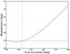 |
Fig. 6 Misalignment Δi between the disk and the binary orbit as a function of the disk inclination (red line) obtained from Eq. (6) for the case of GG Tau A by fixing io = 132.5°, Ωo = 131° and Ωd = 277°. The dashed blue lines mark the values of inclination calculated by assuming the disk to be circular (id = 143°) and the relative misalignment (Δi = 24.9°). |
VLTI/PIONIER and VLT/NACO observations suggest that GG Tau Ab is itself a close binary with two stars with very similar mass at a projected separation of ≈ 4 AU (Di Folco et al. 2014). Given the small separation relative to the distance to the circumbinary disk, which is the subject of our study, we will consider GG Tau Ab1 and GG Tau Ab2 as a single component GG Tau Ab.
Acknowledgments
We kindly thank R. Köhler for providing us with the additional orbits fitted from the astrometric measurements. We also thank S. Facchini and G. Dipierro for the useful discussions, and D. Price for the support with PHANTOM.
References
- Andrews, S. M., Chandler, C. J., Isella, A., et al. 2014, ApJ, 787, 148 [NASA ADS] [CrossRef] [Google Scholar]
- Artymowicz, P., & Lubow, S. H. 1994, ApJ, 421, 651 [NASA ADS] [CrossRef] [Google Scholar]
- Bate, M. R., Bonnell, I. A., & Price, N. M. 1995, MNRAS, 277, 362 [NASA ADS] [CrossRef] [Google Scholar]
- Bate, M. R., Lodato, G., & Pringle, J. E. 2010, MNRAS, 401, 1505 [NASA ADS] [CrossRef] [Google Scholar]
- Birnstiel, T., Dullemond, C. P., & Brauer, F. 2010, A&A, 513, A79 [NASA ADS] [CrossRef] [EDP Sciences] [Google Scholar]
- Birnstiel, T., Klahr, H., & Ercolano, B. 2012, A&A, 539, A148 [NASA ADS] [CrossRef] [EDP Sciences] [Google Scholar]
- Blum, J., & Wurm, G. 2008, ARA&A, 46, 21 [NASA ADS] [CrossRef] [EDP Sciences] [Google Scholar]
- Bonnell, I., Arcoragi, J.-P., Martel, H., & Bastien, P. 1992, ApJ, 400, 579 [NASA ADS] [CrossRef] [Google Scholar]
- Brauer, F., Dullemond, C. P., Johansen, A., et al. 2007, A&A, 469, 1169 [NASA ADS] [CrossRef] [EDP Sciences] [Google Scholar]
- Brauer, F., Dullemond, C. P., & Henning, T. 2008, A&A, 480, 859 [NASA ADS] [CrossRef] [EDP Sciences] [Google Scholar]
- Casassus, S., van der Plas, G., M, S. P., et al. 2013, Nature, 493, 191 [NASA ADS] [CrossRef] [Google Scholar]
- Chiang, E. I., & Murray-Clay, R. A. 2004, ApJ, 607, 913 [NASA ADS] [CrossRef] [Google Scholar]
- Di Folco, E., Dutrey, A., Le Bouquin, J.-B., et al. 2014, A&A, 565, L2 [NASA ADS] [CrossRef] [EDP Sciences] [Google Scholar]
- Dipierro, G., Price, D., Laibe, G., et al. 2015, MNRAS, 453, L73 [NASA ADS] [CrossRef] [Google Scholar]
- Dipierro, G., Laibe, G., Price, D. J., & Lodato, G. 2016, MNRAS, 459, L1 [NASA ADS] [CrossRef] [Google Scholar]
- Doyle, L. R., Carter, J. A., Fabrycky, D. C., et al. 2011, Science, 333, 1602 [NASA ADS] [CrossRef] [MathSciNet] [PubMed] [Google Scholar]
- Duchêne, G., McCabe, C., Ghez, A. M., & Macintosh, B. A. 2004, ApJ, 606, 969 [NASA ADS] [CrossRef] [Google Scholar]
- Duquennoy, A., & Mayor, M. 1991, A&A, 248, 485 [NASA ADS] [Google Scholar]
- Dutrey, A., Guilloteau, S., & Simon, M. 1994, A&A, 286, 149 [NASA ADS] [Google Scholar]
- Dutrey, A., Semenov, D., Chapillon, E., et al. 2014, Protostars and Planets VI, 317 [Google Scholar]
- Elias, J. H. 1978, ApJ, 224, 857 [NASA ADS] [CrossRef] [Google Scholar]
- Facchini, S., Lodato, G., & Price, D. J. 2013, MNRAS, 433, 2142 [NASA ADS] [CrossRef] [Google Scholar]
- Facchini, S., Ricci, L., & Lodato, G. 2014, MNRAS, 442, 3700 [NASA ADS] [CrossRef] [Google Scholar]
- Fischer, D. A., & Marcy, G. W. 1992, ApJ, 396, 178 [NASA ADS] [CrossRef] [Google Scholar]
- Flebbe, O., Muenzel, S., Herold, H., Riffert, H., & Ruder, H. 1994, ApJ, 431, 754 [NASA ADS] [CrossRef] [Google Scholar]
- Foucart, F., & Lai, D. 2014, MNRAS, 445, 1731 [NASA ADS] [CrossRef] [Google Scholar]
- Guilloteau, S., Dutrey, A., & Simon, M. 1999, A&A, 348, 570 [NASA ADS] [Google Scholar]
- Gundlach, B., & Blum, J. 2015, ApJ, 798, 34 [NASA ADS] [CrossRef] [Google Scholar]
- Harris, R. J., Andrews, S. M., Wilner, D. J., & Kraus, A. L. 2012, ApJ, 751, 115 [NASA ADS] [CrossRef] [Google Scholar]
- Hioki, T., Itoh, Y., Oasa, Y., Fukagawa, M., & Hayashi, M. 2011, PASJ, 63, 543 [NASA ADS] [Google Scholar]
- Kennedy, G. M., Wyatt, M. C., Sibthorpe, B., et al. 2012, MNRAS, 421, 2264 [NASA ADS] [CrossRef] [Google Scholar]
- Köhler, R. 2011, A&A, 530, A126 [NASA ADS] [CrossRef] [EDP Sciences] [Google Scholar]
- Kostov, V. B., McCullough, P. R., Hinse, T. C., et al. 2013, ApJ, 770, 52 [NASA ADS] [CrossRef] [Google Scholar]
- Kostov, V. B., McCullough, P. R., Carter, J. A., et al. 2014, ApJ, 784, 14 [NASA ADS] [CrossRef] [Google Scholar]
- Laibe, G., & Price, D. J. 2014, MNRAS, 440, 2136 [NASA ADS] [CrossRef] [Google Scholar]
- Leinert, C., Zinnecker, H., Weitzel, N., et al. 1993, A&A, 278, 129 [NASA ADS] [Google Scholar]
- Lin, D. N. C., & Papaloizou, J. 1979a, MNRAS, 188, 191 [NASA ADS] [CrossRef] [Google Scholar]
- Lin, D. N. C., & Papaloizou, J. 1979b, MNRAS, 186, 799 [NASA ADS] [CrossRef] [Google Scholar]
- Lin, D. N. C., & Papaloizou, J. 1986, ApJ, 309, 846 [NASA ADS] [CrossRef] [Google Scholar]
- Lodato, G., & Facchini, S. 2013, MNRAS, 433, 2157 [NASA ADS] [CrossRef] [Google Scholar]
- Lodato, G., & Price, D. J. 2010, MNRAS, 405, 1212 [NASA ADS] [Google Scholar]
- Lubow, S. H., Martin, R. G., & Nixon, C. 2015, ApJ, 800, 96 [NASA ADS] [CrossRef] [Google Scholar]
- Miranda, R., & Lai, D. 2015, MNRAS, 452, 2396 [NASA ADS] [CrossRef] [Google Scholar]
- Morris, J. P., & Monaghan, J. J. 1997, J. Comput. Phys., 136, 41 [NASA ADS] [CrossRef] [MathSciNet] [Google Scholar]
- Murray, J. R. 1996, MNRAS, 279, 402 [NASA ADS] [Google Scholar]
- Nakagawa, Y., Sekiya, M., & Hayashi, C. 1986, Icarus, 67, 375 [NASA ADS] [CrossRef] [Google Scholar]
- Nelson, A. F., & Marzari, F. 2016, ApJ, 827, 93 [NASA ADS] [CrossRef] [Google Scholar]
- Orosz, J. A., Welsh, W. F., Carter, J. A., et al. 2012a, ApJ, 758, 87 [NASA ADS] [CrossRef] [Google Scholar]
- Orosz, J. A., Welsh, W. F., Carter, J. A., et al. 2012b, Science, 337, 1511 [NASA ADS] [CrossRef] [PubMed] [Google Scholar]
- Paczynski, B. 1977, ApJ, 216, 822 [NASA ADS] [CrossRef] [Google Scholar]
- Papaloizou, J., & Pringle, J. E. 1977, MNRAS, 181, 441 [NASA ADS] [CrossRef] [Google Scholar]
- Pichardo, B., Sparke, L. S., & Aguilar, L. A. 2005, MNRAS, 359, 521 [NASA ADS] [CrossRef] [Google Scholar]
- Price, D. J. 2007, PASA, 24, 159 [NASA ADS] [CrossRef] [Google Scholar]
- Price, D. J., & Federrath, C. 2010, MNRAS, 406, 1659 [NASA ADS] [Google Scholar]
- Raghavan, D., McAlister, H. A., Henry, T. J., et al. 2010, ApJS, 190, 1 [NASA ADS] [CrossRef] [EDP Sciences] [Google Scholar]
- Roddier, C., Roddier, F., Northcott, M. J., Graves, J. E., & Jim, K. 1996, ApJ, 463, 326 [NASA ADS] [CrossRef] [Google Scholar]
- Schäfer, C., Speith, R., & Kley, W. 2007, A&A, 470, 733 [NASA ADS] [CrossRef] [EDP Sciences] [Google Scholar]
- Schwamb, M. E., Orosz, J. A., Carter, J. A., et al. 2013, ApJ, 768, 127 [NASA ADS] [CrossRef] [Google Scholar]
- Shakura, N. I., & Sunyaev, R. A. 1973, A&A, 24, 337 [NASA ADS] [Google Scholar]
- Silber, J., Gledhill, T., Duchêne, G., & Ménard, F. 2000, ApJ, 536, L89 [Google Scholar]
- Simon, M., & Prato, L. 1995, ApJ, 450, 824 [NASA ADS] [CrossRef] [Google Scholar]
- Tang, Y.-W., Dutrey, A., Guilloteau, S., et al. 2016, ApJ, 820, 19 [NASA ADS] [CrossRef] [Google Scholar]
- Von Neumann, J., & Richtmyer, R. D. 1950, J. Appl. Phys., 21, 232 [NASA ADS] [CrossRef] [MathSciNet] [Google Scholar]
- Wada, K., Tanaka, H., Suyama, T., Kimura, H., & Yamamoto, T. 2009, ApJ, 702, 1490 [NASA ADS] [CrossRef] [Google Scholar]
- Welsh, W. F., Orosz, J. A., Carter, J. A., et al. 2012, Nature, 481, 475 [NASA ADS] [CrossRef] [PubMed] [Google Scholar]
- Welsh, W. F., Orosz, J. A., Carter, J. A., & Fabrycky, D. C. 2014, in IAU Symp. 293, ed. N. Haghighipour, 125 [Google Scholar]
- Whipple, F. L. 1972, in From Plasma to Planet, ed. A. Elvius, 211 [Google Scholar]
- White, R. J., & Ghez, A. M. 2001, ApJ, 556, 265 [Google Scholar]
- White, R. J., Ghez, A. M., Reid, I. N., & Schultz, G. 1999, ApJ, 520, 811 [NASA ADS] [CrossRef] [Google Scholar]
Appendix A: Dependence of the final gas density profile on the temperature profile
The temperature profile in Eq. (4) is very steep. We therefore also check how the assumed temperature profile affects the steady state gas density profile and the location of the dust trap. For the coplanar case, we compare the density profiles resulting from the hydrodynamical simulations assuming the temperature profile calculated by Guilloteau et al. (1999) (T ∝ R-0.9) and a less steep and more common T ∝ R-0.5 profile in the case of α = 0.01. The two profiles are shown in Fig. A.1. In particular, we assume the temperature profile  (A.1)where the temperature at 300 AU is fixed to 20 K, as in Guilloteau et al. (1999).
The T ∝ R-0.5 profile leads to a steeper gas density profile, and the location of the density peak is located at smaller radii with respect to the T ∝ R-0.9 case. This shows that a less steep temperature profile does not cause an increase in the radius of the ring and that, even under the hypothesis that T ∝ R-0.5, a misalignment between the plane of the disk and that of the orbit is needed in order to explain the location of the mm-sized dust ring.
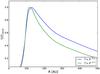 |
Fig. A.1 Azimuthally and temporally averaged gas radial density profiles, obtained using α = 0.01 and two different temperature profiles. As expected, the density profile resulting from the T ∝ R-0.5 is steeper than the T ∝ R-0.9 profile, and the density maximum in the first case is even farther away from the observed dust location (~ 200 AU) than in the latter case. Both density profiles are normalized to their maximum values. |
All Tables
All Figures
|
Fig. 1 Observational constraints available to date for different sized grains and for CO distribution. The gray-shaded area shows the 2σ uncertainty on the mm-sized dust radial density profile as modeled in Andrews et al. (2014). The red dash-dotted and the green dashed lines show the radial extent of CO and micron-sized dust grains, respectively. It should be noted that these two tracers are optically thick and do not provide information about the density profile. The vertical location of the lines is therefore arbitrary. |
| In the text | |
|
Fig. 2 Azimuthally averaged gas density profile for the α = 0.002 simulation at different evolutionary stages. After a few hundred binary orbits the density profile reaches a quasi-stationary configuration. All the density profiles are normalized to the maximum of the density profile at the end of the simulation. |
| In the text | |
|
Fig. 3 Gas density profiles obtained from our simulations (solid lines) in the coplanar case using α = 0.01,0.005,0.002. The gas density profile invoked by Andrews et al. (2014) is also plotted (dashed line) for comparison. |
| In the text | |
|
Fig. 4 Snapshot of the inner cavity of the circumbinary disk at 1000 binary orbits in the α = 0.002 case. The white dots indicate the location of the two central stars; the dashed lines show the location of the pressure maximum. The image was produced using SPLASH (Price 2007). |
| In the text | |
|
Fig. 5 Density profiles for gas (solid red line) and dust (solid blue for mm-sized and solid green for micron-sized) obtained from our simulations in the coplanar case using α = 0.002. The gas and dust density profiles from the model by Andrews et al. (2014) are also plotted (dashed lines) for comparison. It is clear that the solid blue line showing the mm-sized dust surface density profile is not consistent with the data (gray shaded area). |
| In the text | |
|
Fig. 6 Misalignment Δi between the disk and the binary orbit as a function of the disk inclination (red line) obtained from Eq. (6) for the case of GG Tau A by fixing io = 132.5°, Ωo = 131° and Ωd = 277°. The dashed blue lines mark the values of inclination calculated by assuming the disk to be circular (id = 143°) and the relative misalignment (Δi = 24.9°). |
| In the text | |
|
Fig. A.1 Azimuthally and temporally averaged gas radial density profiles, obtained using α = 0.01 and two different temperature profiles. As expected, the density profile resulting from the T ∝ R-0.5 is steeper than the T ∝ R-0.9 profile, and the density maximum in the first case is even farther away from the observed dust location (~ 200 AU) than in the latter case. Both density profiles are normalized to their maximum values. |
| In the text | |
Current usage metrics show cumulative count of Article Views (full-text article views including HTML views, PDF and ePub downloads, according to the available data) and Abstracts Views on Vision4Press platform.
Data correspond to usage on the plateform after 2015. The current usage metrics is available 48-96 hours after online publication and is updated daily on week days.
Initial download of the metrics may take a while.