| Issue |
A&A
Volume 599, March 2017
|
|
|---|---|---|
| Article Number | A143 | |
| Number of page(s) | 14 | |
| Section | Numerical methods and codes | |
| DOI | https://doi.org/10.1051/0004-6361/201629719 | |
| Published online | 16 March 2017 | |
Stellar halo hierarchical density structure identification using (F)OPTICS
Instituut voor Sterrenkunde, KU Leuven, Celestijnenlaan 200D, 3001 Leuven, Belgium
e-mail: This email address is being protected from spambots. You need JavaScript enabled to view it.
Received: 14 September 2016
Accepted: 23 November 2016
Abstract
Context. The stellar halo holds some of the best preserved fossils of Galactic formation history that can be detected as overdensities. The detection and analysis of merger by-products within the halo enables the reconstruction of the accretion history of the Milky Way. Upcoming large-scale all-sky surveys such as Gaia and The Large Synoptic Survey Telescope (LSST) will provide a huge and rich data set, which at the same time poses challenges for automated halo debris detection.
Aims. We investigate the overdensity detection algorithm Ordering Points To Identify the Clustering Structure (OPTICS) as a method to identify tidal debris in the Galactic halo with large-scale surveys, as well as the variant FOPTICS which is capable of handling data sets with multi-dimensional uncertainty ellipsoids.
Methods. We applied OPTICS to the a simulated Galactic stellar Halo to assess the detection performance. Additionally, we tested the performance of FOPTICS is tested by introducing uncertainty ellipsoids to the 6D phase space of two test cases. We present the Jaccard index as an alternative way to test the stability of halo debris overdensity detections without the need for a local background density estimate.
Results. We optimized the OPTICS overdensity detection algorithm so that it has a slightly superlinear run-time complexity, making the method suitable for large-scale surveys. Our test on a mock galactic halo in 6D phase space shows an excellent capability to not only detect the compact dense clusters, but also the larger streams that cover a significant part of the sky. The output of OPTICS, the so-called 2D reachability diagram, proved to be a very useful tool to grasp the size, density, and substructure of the overdensities without needing to resort to complex projections of the 6D phase space. Using FOPTICS, we show the effects of introducing uncertainty ellipsoids in the 6D phase space on the retrieved tidal streams, and how the detectability of a cluster depends on whether its size and density is sufficiently large to overcome the effects of the uncertainties on the attributes.
Key words: Galaxy: structure / Galaxy: halo / techniques: miscellaneous / methods: numerical
© ESO, 2017
1. Introduction
Following the discovery of a “large, extended group of co-moving stars in the direction of the Galactic Center” by Ibata et al. (1994), and the advent of large all-sky photometric surveys such as SDSS and 2MASS, the search for galactic merger remnants has boomed. These merger by-products, in the form of stellar streams, stellar overdensities and globular clusters, are the results of gravitationally disrupted satellites and are ubiquitous in hierarchical cosmological simulations (Bullock & Johnston 2005; Helmi 2008; Johnston et al. 1996; Bullock et al. 2001). The detection of these stellar streams, stellar overdensities, and globular clusters with narrow extended tails, provides evidence that the stellar halo is abundantly structured. Furthermore, the existence of such structures indicates that the Milky Way has undergone an extensive accretion history during its formation (Helmi 2008). The continued detection and analysis of merger by-products within the halo will enable the reconstruction of the accretion and formation history of the Milky Way, in the near future.
While the visual detection of merger remnants has been exceedingly successful, the shear volumes of data which are expected to become available in the immediate future will make visual inspection no longer feasible. Large-scale all-sky surveys such as Gaia (Perryman 2002), LSST (Ivezić et al. 2008), and SkyMapper (Keller et al. 2007) are expected to deliver unprecedentedly large and more complex data sets, exceeding six-plus dimensions for billions of stars. The seemingly overwhelming task to detect stellar overdensities in the stellar halo in multiple observational dimensions has began its migration toward automated data mining techniques.
Although many cluster detection algorithms exist in the field of data mining, many of them do not meet the requirements for halo overdensity detection. For the latter, no a priori information on the number of overdensities is available; overdensities may not be linearly separable, need not be compact, can be stream-like, can show substructure, and are always embedded in a background that shows a density gradient. Moreover, the search is preferably done in more than three dimensions and the number of stars involved can easily be more than several million, putting strong constraints on the computational performance. To meet these challenges, several dedicated clustering algorithms have been developed and published in the astronomical literature; see for example, ISODEN (Pfitzner et al. 1997), SUBFIND (Springel et al. 2001), 6DFOF (Diemand et al. 2006), HSF (Maciejewski et al. 2009), ENLINK (Sharma & Johnston 2009), and ROCKSTAR (Behroozi et al. 2013). For a comparison of several of the above mentioned algorithms, see Knebe et al. (2011) and Elahi et al. (2013).
In this paper we assess the performance of two closely related algorithms for overdensity detection in the Galactic halo. The first, Ordering Points To Identify the Clustering Structure (OPTICS) is a multi-dimensional hierarchical density-based clustering algorithm developed originally by Ankerst et al. (1999) with the ability to detect clusters with large density variations against a background. As such, OPTICS is specifically designed to detect overdensities against a non-uniform background, small-scale substructures in large-scale overdensities, and irregular shaped clusters such as streams and clouds. Secondly, Fuzzy Ordering Points To Identify the Clustering Structure (FOPTICS) is a generalized version of OPTICS that was developed by Kriegel & Pfeifle (2005), which enables the clustering of fuzzy data sets: i.e. data sets whose objects are defined by means of probability density distributions rather than infinitely precise point sources.
Given that so many overdensity detection algorithms are already available, why is there a need to introduce yet another one? There are two aspects in which the current algorithms in the astronomical literature often underperform and in which OPTICS makes significant progress. The first aspect concerns a comprehensive visualization of the overdensities. Although such a visualization is not strictly necessary to detect overdensities, it makes the analysis far easier and practical. As a hierarchical clustering algorithm, OPTICS output (a reachability diagram) is similar to the classic dendrogram. Such a reachability diagram allows the arrangement of structure and substructure of halo overdensities in a six-dimensional phase space to be visualized in a comprehensive two-dimensional representation.
The second aspect, which is more important astrophysically, OPTICS can be adapted in a natural way to include uncertainties of the attributes, giving rise to FOPTICS. In the case of the Galactic halo, for example, the position in the sky is (usually) more accurately known than the distance of the star, especially for the outer halo. The velocity components can have a larger relative uncertainty than the geometrical position. As a result, halo overdensities can be a lot fuzzier, i.e., the have a more extended probability distribution in one dimension than in another. For the remainder of this article, we adopt the word fuzzy to refer to any quantity with associated uncertainties. A good overdensity detection algorithm should take these uncertainties into account. For example, stars in a more distant part of a stream can have larger uncertainties than those in a nearby region, warranting more caution to define the extent of the distant part. As another example, two overdensites that are deemed close, but separated in phase space, may not be separable at all when taking the uncertainties into account.
This article aims to answer some of the following open questions. Although OPTICS and FOPTICS look promising on paper, how well do they perform on multi-dimensional halo data? To what extent are these methods useful and what are their limitations? More importantly, can we develop a version of the algorithm that is fast enough to cope with Gaia-like quantities? The paper is structured as follows. We first briefly explain how OPTICS works and how one can interpret its output. In the following section we explain the implemented optimizations used to accelerate the algorithm. Next, we assess the performance of the algorithm using 6D phase space data of a mock galactic halo for which we can compare the OPTICS output with the known solution. Finally, we introduce uncertainties on the mock galactic halo data to investigate the performance of FOPTICS.
2. Identifying the clustering structure
2.1. The OPTICS algorithm
Before briefly summarizing the algorithm, we introduce some definitions needed to explain how OPTICS identifies the clusters. Given a sample S of L points, each having Natt attributes (position, velocity, ...), OPTICS defines around each point p an, ε-neighborhood Nε(p), which is the set of points within a multi-dimensional Euclidean distance ε of p. Formally the ε-neighborhood,  (1)If the ε-neighborhood contains at least a minimum number of points Nmin, the point p is said to be a core point pc, i.e. composing part of the cluster core. Every core point has a corresponding core distance, dc, which is defined as the distance to the Nmin-th closest neighbor, which is always dc ≤ ε. If there are less than Nmin points in the ε-neighborhood, dc remains undefined.
In addition, the reachability distance of a point p is the Euclidean distance to the nearest core point pc, d(p,pc) or the core distance of pc, whichever is larger, i.e.,  (2)Since the reachability distance is always defined with respect to a previously identified core point pc, if dc is undefined, dr is undefined as well. Therefore, an OPTICS defined cluster is a group of points that are linked through a series of ε-neighborhoods and must contain at least one core point and Nmin points.
To cluster a given data set, the OPTICS algorithm passes once over the whole data sample, iteratively ranking points based on minimum reachability distance. Starting from an arbitrary point p in the data set, the algorithm retrieves the ε-neighborhood of p and determines whether it is a core point or not. If so, the algorithm calculates and sorts the reachability distances dr of all its neighbors, choosing the neighbor with the smallest dr as the next point in the processing order. If this new point is a core point as well, its neighbors are also added to the neighborhood set and both its dr and dc distances are added to the ranking. The process is continued until all members of the neighborhood set have been processed and their associated dr and dc distances added to the ranking. Once the neighborhood set becomes empty, the algorithm moves on the next unprocessed point of the sample and continues processing the remaining objects until all objects in the sample have been visited.
2.2. The reachability diagram
The result of OPTICS is an ordered set of points in which the processing order, dr, and dc for each object are stored. A graphical representation of the processing order versus reachability distance (order versus dr) is known as a reachability diagram. The reachability diagram is one of the major benefits of OPTICS over other currently available clustering algorithms. The exact structure of this diagram depends on the parameters ε and Nmin, which in turn depends on the scientific question at hand; but our experience shows that the overall shape of the reachability diagram does not change when the input parameters are varied within 20%.
We created, clustered, and extracted a two-dimensional data set, to illustrate the functionality of the OPTICS algorithm and in particular the strength of the reachability diagrams. The data set, whose two-dimensional distribution is shown in the top panel of Fig. 1, contains five clusters. Each cluster was designed to exhibit individual characteristics that are similar to clusters found in the stellar halo (i.e., varying density, irregular shapes, and elongated tails). The associated reachability diagram is shown in the bottom panel of Fig. 1. In this reachability diagram, and in the rest of this article, we present the normalized reachability distances, Dr, which range from 0 to 1, and are calculated as  (3)The clusters and associated portions of the reachability diagram were color-coded based on the cluster extraction method described in Sect. 2.3.
By definition clusters are regions of multi-dimensional space where reachability distances between points are small. Within the reachability these areas of low Dr correspond to a high-density region that is associated with clusters and substructure within the clusters. As a result, each clusters is enclosed by two high Dr-value (low density) border points. These peaks are indicative of transition regions between clusters and/or areas of low density (i.e. the background) where the reachability distances are undefined and set to Dr = 1.0.
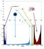 |
Fig. 1 Top panel: two-dimensional cluster distribution used to produce the reachability diagram below. Bottom panel: associated reachability diagram, order vs. the normalized reachability distance Dr, resulting from applying OPTICS to the above data set. The color coding and arrows indicate the location of each cluster within the reachability diagram. |
While OPTICS does not explicitly produce a clustered structure, this structure can easily be extracted from the reachability diagrams, as described in Sect. 2.3. The size of the derived clusters is given by the number of points contained between two peak values, while the relative density is given by the depth of each valley. Large and dense clusters with nearly symmetric density profiles span a large fraction of the reachability diagram at relatively low and constant reachability distances. This behavior is typical of a multi-dimensional Gaussian as shown by the cluster in light blue in Fig. 1. Inversely, smaller clusters cover smaller regions of the reachability diagram and sparse clusters have relatively high Dr values. Since the internal density variations within the clusters result in varying Dr, the values in the reachability diagram may contain small sub-valleys of their own, indicating parts of the cluster where the density is even higher.
Because of the OPTICS processing order, where the object with the smallest reachability distance is always processed first, the algorithm always finds the densest part of the nearest cluster before continuing to build the clustering structure of the data set. The resulting exact shape of a cluster valley in the reachability diagram depends on the multi-dimensional density distribution of the cluster. We note that because OPTICS is a hierarchical algorithm, the algorithm used to extract clusters from the reachability diagram always returns only the deepest portions of the valleys (i.e., the final leaves of the hierarchical tree). In some cases, as shown by with the last cluster in red of Fig. 1, the outer boundaries of clusters are not extracted despite clearly belonging to a reachability valley, see Sect. 2.3 for more details.
2.3. Cluster extraction
The visual inspection of reachability diagrams can prove insightful and can be performed rather quickly for small data sets. For large data sets, on the other hand, an automated extraction method is required, particularly if the clusters are to be used as a preprocessing step for other data mining algorithms. Sander et al. (2003) introduced an automatic clustering extraction algorithm for hierarchical clustering representations as a method of converting a reachability diagram into a hierarchical tree (dendrogram) and vice versa. Since dents in the reachability diagram, associated with clusters, are separated by regions of higher reachability, the algorithm is based on the identification and sorting of local maxima. We present a modified version of the Sander et al. (2003) algorithm for the cluster extraction, in which the possible entrance and exit boundaries of clusters are not solely defined as local maxima but are defined by two sets of criteria as described in the following.
The extraction algorithm provides concise and accurate results through the identification of cluster entrance and exit border points. The algorithm defines all possible transition points (local entrance and exit points) using two sets of criteria and sorts them according to decreasing Dr value. Assuming the point in question is identified in the processing order as point i and that a cluster must contain at least Nmin points, the set of possible local entrance points is defined as all points that satisfy the following conditions:  where Dri is the reachability distance value of the possible local point. Similarly, the set of all possible local exit points is composed of all objects that satisfy the inverse conditions:
  However, not all regions enclosed by two local border points are prominent clusters. In order to identify if any given region is a prominent cluster, the algorithm checks whether a split of the data set at each of the combinations of local border points would return two clusters, both of which contain at least Nmin points and have an average reachability distance that is significantly different from the reachability of the current local border point. If both conditions are not satisfied, the local border point in question is removed from the list and the algorithm continues to the next highest local border point, assuming the next highest local border point exceeds a minimum threshold Tmin. This threshold identifies the lowest possible local border point which could form a prominent cluster to avoid the detection of superfluous smaller clusters. If a split at the current local border point results in two clusters both of which satisfy both conditions, the algorithm continues to check whether the cluster is a subcluster of a larger previously detected cluster or is significantly similar in size and density to any of the previously detected clusters. This similarity condition checks how similar the size and mean reachability distance of each cluster is compared to that of the previously detected parent clusters. If either the ratio of sizes (S):
  (8)or the ratio of the mean reachability (R):
  (9)exceed a specific user defined similarity ratio, Ts, the current cluster Ci is considered significantly similar to a parent cluster Cp and the node is moved up in the tree and becomes a possible parent cluster. As a result, the depth of the clustering extraction depends on the two parameters, Tmin and Ts. Our tests indicate that for large data sets with an exponentially decreasing background, Tmin should be set between 0.01 and 0.1, depending on the structure and density of the data set. For the applications in this paper, we chose Tmin = 0.025 after visual inspection of the reachability diagrams.
Furthermore, Sander et al. (2003) notes that the extraction also depends on Ts, as it allows for the differentiation between small-scale and large-scale structures. Inversely, a higher value of Ts dictates that the clusters are very similar but still satisfy the extraction criteria individually. As a result, clusters that contain substructure whose internal properties are significantly different may independently satisfy the extraction criteria. This type of behavior becomes immediately clear in the color–coded reachability diagrams, where substructures within valleys are independently identified while the outer borders of the clusters are ignored by the extraction algorithm. Modification of the extraction parameters, in particular the a decrease of Ts results in the omission of such substructure from the extracted clusters. Finding the appropriate Ts value for any given data set and given science goals is therefore a delicate balance between detecting many small (sub)clusters (i.e., only detecting substructure) and detecting only large-scale structures. For the purpose of detecting individual large-scale structures as presented here, we find that a value greater than or equal to 0.1 results in a useful extraction of the density structure, without overcompensating for possible noise-like substructures. A much lower value of TS results in the over-splitting of clusters into much smaller substructures.
2.4. Cluster significance and stability
For any large data set a number of small clusters may appear as a result of noise in the background. We expect these insignificant clusters to have low ΣDr values. One approach is therefore to apply a Monte Carlo approach that derives the distribution of ΣDr values given a Poisson background, which can then be used to derive a cluster significance test.
Clearly this requires a reliable local background density estimate; a cluster dense and large enough to be significant in the sparse outer halo, may not be significant in the inner halo which has a denser background. Such approach is therefore only expected to work reasonably well in the case of small isolated clusters, for which reliable background estimates can be determined. The method fails, however, when we are dealing with large stream-like clusters that extend over a range of background densities.
An alternative approach we explore is the notion of cluster stability. The cluster stability assesses how stable a cluster extraction is against small changes in the original data sample and gives an indication of the reliability of the clusters. In this respect, stability acts as a proxy to significance, since a more stable cluster is typically also more significant. In what follows, we adopt the methodology presented in Hennig (2007) for testing the cluster stability. The procedure requires the derivation, clustering and extraction of a series of new samples; in which a sample is derived from the original data set using bootstrapping (drawing with replacement) while maintaining the original sample size. The clustering results of the original sample are then compared with the clustering results of the newly derived sample. If a cluster present in the original sample is also largely present in the bootstrapped sample, the cluster is deemed stable. Inversely, if a cluster largely disintegrates in the new sample, it is considered unstable. To quantify the stability of a clusters we use the Jaccard coefficient, also known as the Jaccard similarity or Jaccard similarity index (Hennig 2007). More recently, the method has proven to outperform subsampling as a method of finding the “true” number of clusters (Mucha et al. 2015; Hofmans et al. 2015).
The concrete procedure used to determine the stability of our extracted clusters is as follows. We created K bootstrap samples of the same size as the original sample, and applied OPTICS to extract the clusters. Because of the bootstrapping, some stars are completely omitted, while others occur multiple times within the newly created Ki sample; effectively changing the overdensity structure of the data set. To determine which cluster of the bootstrapped sample corresponds to which cluster in the original sample, we compute the Jaccard similarity index for all possible combinations of the originally detected cluster (CO) and all clusters detected within the bootstrapped samples (CS), such that  (10)The cluster combination CO−CSi with the largest Jaccard index,
  (11)is assumed to indicate a match. Repeating this process over all K samples, a distribution of Jaccard indices per cluster is created, which describes how well the cluster remains stable throughout the different bootstrapped samples. Finally, the average
  of the K (maximum) Jaccard indices are computed as a measure for the stability of cluster Ci. Values close to one indicate very stable clusters; values close to zero indicate that bootstrapping almost always causes the cluster to disintegrate in the background. In practice, we find that K = 50 bootstrapped samples are sufficient to obtain a reliable average Jaccard index. We present a concrete application and assessment of this method in Sect. 4 on a mock stellar halo.
3. Performance optimization for large surveys
If a halo overdensity detection algorithm is to be applied to large surveys, of a few million point sources, such as Gaia, it must be able to process large data volumes quickly. We have made a considerable effort to optimize the OPTICS time complexity. In Ankerst et al. (1999), ε is defined as the radius of a D-dimension hypersphere containing at least Nmin number of objects under the assumption that the data set is uniformly distributed and covers the same multi-dimensional volume as the data set to be clustered. This becomes a problem with high-dimensional data sets or data sets with large variances or exceptional outliers which can cause the multi-dimensional volume to be extremely large. In such situations the use of ε as estimated by Ankerst et al. (1999) can result in ε being exceptionally large, up to and including the whole data set. Given the total number of N-points in a sample, and the run-time rε of one ε-neighborhood query, the run time of OPTICS is approximately  and depends strongly on the multi-dimensional structure of the data set. In cases where the ε-neighborhood includes the whole data set, the run-time complexity can become as high as
  .
.
However, with some optimizations the OPTICS run time can be dramatically reduced. For most applications, Ankerst et al. (1999)ε-neighborhood only covers a small fraction of the entire volume of the data set. Since Nmin is usually much smaller than the total number of points L, this implies that for each ε-neighborhood query, a large fraction of the data set falls outside the hypersphere and can be ignored. We are able to exceptionally speed up OPTICS by avoiding to compute distances for objects outside the ε-neighborhood, since distance computations are CPU intensive.
Given the increasingly large data volumes, several optimization methods exist, such as tree structures and hashing, which are currently active research topics. While the use of such methods can show great improvement in the run-time of algorithms, no method is optimal for all problems or algorithms. In the case of OPTICS, the performance of the algorithm depends heavily on the spatial structure of the data set.
We developed a fast nonparallel FORTRAN version of OPTICS with the goal to make the application to large data sets feasible even on desktop computers. It has been tested successfully on data sets of up to a few million six-dimensional points.
To investigate the total run-time complexity of our implementation of OPTICS, we simulated several data sets. Each of these data sets were drawn from a uniform distribution within a six-dimensional hypercube. We used a value of Nmin = 50, and adapted ε accordingly so that on average Nmin points are present within a hypersphere of radius ε. Figure 2 shows the resulting run-time in function of the data set size in log-log scale. A linear least-squares fit of the run-time data results in a slope of 1.16 indicating a complexity very near to  . In the case of complexity, the resulting slope would be 2.
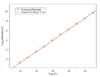 |
Fig. 2 Run time complexity of our implementation of OPTICS shown in Log-Log scales. The red line indicates the linear least-squares fit, whose slope is 1.16, indicating a near linear complexity. |
The slight deviation from linearity is caused by the spatial grid structure used in the optimization of OPTICS as described below. For an increasing number of bins, the complexity becomes asymptotically linear for two reasons. The data points in grid cells at the borders of the data set require less computation time given that they have a smaller number of epsilon-neighborhood candidates and simultaneously, the number of points residing in “border” cells decreases with increasing grid density.
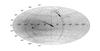 |
Fig. 3 Aitoff projection of all 483 733 objects, composing a total of 74 unique clusters, used to cluster Halo-02. |
The following optimizations have been implemented to obtain the previously mentioned nearly linear complexity:
-
Seed
list optimization:
OPTICS uses a sorted seed list to deter-mine the point with the minimum reachability distance; thesubsequent point to be processed. Managing the list using binarytrees reduces the computation time required to find the subse-quent point. Instead of continuously sorting and addressing thefirst object in the array, we build a binary tree of the reachabilitieswhose root node is by definition the smallest reachability dis-tance; the brute-force approach would require looping over theentire seed list every time a new object is queried. Once the small-est reachability distance is extracted, the tree is rebuilt includingthe reachability distance of all newly added points. These oper-ations are much less CPU-intensive than looping over the entireseed list every time or even using quick-sort routines.
-
Spatial
gridding and hashing:
every point in a multi-dimensional data set has multi-dimensional coordinates. The data space is split into equally spaced multi-dimensionally indexed data cubes (whose volumes are εD) and a hashing function is used to assign a unique integer value to the multi-dimensional index. This enables the algorithm to calculate distances to only points belonging the directly neighboring bins, thereby reducing the number of distance calculations needed to determine the ε-neighborhood of any given point.
-
Partial sorting:
sorting large arrays is computationally expensive. We use a partial sorting method to accelerate the core distance determination. Instead of sorting all members of the ε-neighborhood, only the Nmin objects with the smallest distances are returned in a sorted order. This allows for the algorithm to avoid excessive and expensive computations in the determination of the core-distance of any given object, especially if the ε-neighborhood is large.
While these optimizations work extremely well to speed up OPTICS, they do not apply to the FOPTICS version of the code (See Sect. 5), where the ε-neighborhood of each object must contain the entire data set. While we were able to decrease the run-time complexity of OPTICS to nearly , the run-time complexity for FOPTICS remains  ), with M being the number of samples used to estimate the uncertainty distributions. As a result, the typical sample sizes for which FOPTICS can be applied are smaller than those of OPTICS. Kriegel & Pfeifle (2005) provide more detailed description of the computational aspects of FOPTICS.
4. Assessment on a mock stellar halo
4.1. Overdensity detection
To assess the performance of OPTICS on clustering large data sets, similar to those that are expected to become available in the immediate future with Gaia, we work with the Bullock & Johnston (2005) simulated Galactic Halo-02 sample. Halo-02 consists of 2 million points distributed into 115 clusters, which extend radially to distances of 150 Mpc from the Galactic center. Each point is described by a six-dimensional phase-space position in Cartesian coordinates (position in [kpc] from the Galactic center and velocity in [km s-1]) and an associated cluster number alongside synthetic u−z SDSS magnitudes (Bullock & Johnston 2005; Robertson et al. 2005; Font et al. 2006a,b). We have downscaled the Halo-02 data set to 483 733 objects contained within 85 kpc of the Galactic center and distributed into 74 clusters, whose synthetic magnitudes places them within the Gaia observable magnitude range of 3 < G < 20. The Aitoff projection of this sample is shown in Fig. 3.
This synthetic halo contains overdensities of various sizes and concentrations, as well as streams covering large portions of the sky some of them overlapping in multiple dimensions. Also, most of the clusters (50 out of the 74) are so spread out over the sky and are no longer recognizable as a localized overdensity, but form a diffuse background.
The OPTICS algorithm calculates the distance between points using a multi-dimensional Euclidean distance. For the above mentioned data set, we chose to perform the clustering in phase space, but with the coordinates normalized using Eq. (3). Using this distance, we applied OPTICS using a minimum overdensity size of Nmin = 50 and extraction parameters Ts = 0.01 and Tmin = 0.15.
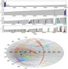 |
Fig. 4 Top panel: reachability diagram produced by OPTICS when clustering the down-scaled Halo-02 sample. As per definition, the x-axis represents the processing order derived from OPTICS and the y-axis gives the normalized reachability (Dr) where dr has been normalized to the highest defined value and all undefined values set to one. Bottom panel: Aitoff projection of objects used in the clustering of Halo-02. Each extracted cluster was color coded to show its location in both the reachability diagram and the Aitoff projection. Comparing Fig. 3 and the Aitoff projection presented here it is clear that OPTICS recovers all of the clusters that are visible by eye. More importantly, OPTICS is able to disentangle clusters that appear to overlap in their Aitoff projections. |
4.2. Validation
The result of the OPTICS application on the mock galactic halo is shown in the reachability diagram in Fig. 4. The many valleys correspond to the different detected overdensities and streams. In the bottom panel of Fig. 4 an Aitoff projection is shown with the same color coding as used in the reachability diagram.
The sky map shows that OPTICS performs very well in identifying the different streams and clouds against a background. In total, 88 overdensities were detected. These do not correspond one-to-one to the 74 original clusters, but come from (portions of) 24 original clusters. As mentioned before, the remaining 50 original clusters form a diffuse halo background in which OPTICS succeeded in detecting the localized overdensities. Many of the 24 original clusters simulated by Bullock & Johnston (2005) are tidally deformed into a string of no longer firmly gravitationally bound overdensities, and/or are very close to other clusters, and/or are wrapped around the Galactic center multiple times. These clusters were identified by OPTICS as a series of smaller clusters that can be traced back to one original cluster. An example of this is shown in Fig. 5, where we show the X-Y projections of CT streams 63 and 33. Because of the internal density variation in the stream, and the overlap with other overdensities, OPTICS detected these two streams as a series of smaller partitions. We overplotted the different regions in red to give an overview of the extracted structure. However, we did not overplot the background or nearby overdensities for the sake of clarity. In Fig. 6 we show the correspondence between the 88 clusters extracted by OPTICS (CO) and the 24 detected true clusters (CT) listed by Bullock & Johnston (2005). The figure shows that associated parts are largely consecutively detected in the reachability diagram, which could be exploited to aggregate smaller clusters into a supercluster.
To quantify the crossmatch between the OPTICS clusters and the Bullock & Johnston (2005) ones, we first find out for every cluster CO extracted by OPTICS, which true cluster CT overlaps most. We can then define:
-
the number of true positives: NTP = #(CO ∩ CT);
-
the number of false positives: NFP = #CO−NTP;
-
the number of false negatives: NFN = #CT−NTP;
-
the completeness: NTP/ (NTP + NFN);
-
the contamination: NFP/ (NTP + NFP).
We also compute for each of the 74 detected true clusters CT which fraction of its stars is part of any one cluster extracted by OPTICS, 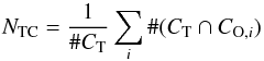 (12)where CO,i are the clusters extracted by OPTICS, and where the subscript “TC” stands for “total completeness”. The results are summarized in Figs. 7 and 8.
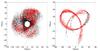 |
Fig. 5 X-Y projections of Bullock & Johnston (2005) overdensity 63 (left) and overdensity 33 (right) are plotted in black. The OPTICS partitions are overplotted in red. The other overlapping overdensities are not plotted for the sake of clarity, but are the main reason the completeness is not 100%. |
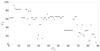 |
Fig. 6 Identification numbers of the clusters CO detected by OPTICS vs. the identification numbers of the true clusters CT with the largest overlap. Sometimes a true cluster is detected by OPTICS as multiple clusters. This simply indicates that the chain of ε-neighborhoods connecting two or more sections of the same cluster has been broken due to poorly connected parts or because a part was assigned to another strongly overlapping cluster. |
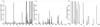 |
Fig. 7 Left-hand panel: completeness of each cluster CO extracted by OPTICS with respect to the original cluster CT given by Bullock & Johnston (2005). The low values are because many streams experienced a tidal breakup, and the individual partitions detected by OPTICS were compared with the entire stream size. Right-hand panel: what fraction of true clusters show up in any cluster extracted by OPTICS. Many overdensities are recovered with a large total completeness. Some of the low total completeness values come from clusters that are so sparse compared to the background that they are difficult to distinguish. The middle panel shows the contamination in each cluster extracted by OPTICS. |
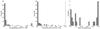 |
Fig. 8 Left-hand panel: histogram of the completeness the OPTICS extracted cluster (CO). It is clear that a large fraction of our detected clusters have low completeness values, as explain in the caption of Fig. 7 and in the text. Middle panel: contamination histogram, where it is obvious that the vast majority of our detected clusters have contamination rates of less than 10%. Right-hand panel: histogram of what fraction of true clusters show up in any cluster extracted by OPTICS. A dichotomy is can be seen in this panel, where clusters are either very well recovered or only a small fraction are detected. The low total completeness values come from clusters that are so sparse compared to the background that they are difficult to distinguish. |
Since most clusters detected by OPTICS are part of a stream, and since the completeness was computed by normalizing with the size of the entire stream size, we can expect low completeness values for the individual parts, as shown in the left-hand panel. If we add up the different parts of the same stream, and then compute the “total” completeness, the values are much higher, as is plotted in the right-hand panel; 11 clusters have a completeness greater than 60% of which 8 have a completeness rate greater than 90%. From the contamination in the middle panel, it can be seen that the cluster extraction algorithm is conservative: it will not easily pollute the detected overdensities with background stars.
Our results indicate that large and extended clusters, such as streams, as well as more concentrated structures such as globular clusters and dwarf galaxies can be successfully recovered with OPTICS, albeit sometimes in multiple smaller partitions.
4.3. Stability
We test the stability of our clusters using the Jaccard similarity index as described in Sect. 2.4. We created 50 bootstrapped samples of our 483 733 object sample, on which we ran OPTICS. The stability coefficient (i.e. the averaged maximum Jaccard index  ), is reported in Fig. 9 for all clusters detected in the original sample. As expected we find that the largest clusters remain completely stable with little variation in the inclusion/exclusion of member stars during the procedure, while smaller clusters are often diffused into the background or split into multiple parts unless they are sufficiently dense. A total of 63 clusters remain relatively stable to a level of 0.5 or greater of which 10 remain completely stable to a level of 0.9. All clusters with a stability index lower than 0.5 are considered unstable. These clusters disintegrated (partly or completely) into the background or are broken up in two or more subclusters for a substantial number of bootstrap samples. The latter indicates that the cluster as a whole cannot be considered stable.
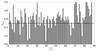 |
Fig. 9 Stability index for each of the extracted clusters in the original sample. The black line indicates a cutoff limit of 0.5. 63 Clusters are above this cutoff limit that can be considered significant and stable. |
5. Identifying a fuzzy clustering structure
5.1. The FOPTICS algorithm
Unlike simulated uncertainty-free data, astronomical data sets are subject to uncertainties. They consist of multi-dimensional and often correlated uncertainties due to observational and instrumental errors. Fuzzy Ordering Points To Identify the Clustering Structure (FOPTICS) is a generalized version of OPTICS that allows for the inclusion of uncertainties within a data set (Kriegel & Pfeifle 2005). Unlike OPTICS, FOPTICS no longer works with infinitely precise attributes, but rather searches for overdensities in attribute probability density distributions. This requires the use of probability density distributions in the formulation of the core distance and reachability distance, as objects are no longer described by a single multi-dimensional position but rather by multivariate distributions. For a complete derivation of the fuzzy core distance and fuzzy reachabilities see Kriegel & Pfeifle (2005).
Given that neither the fuzzy core distances nor the fuzzy reachability distances can be computed analytically, FOPTICS uses a Monte Carlo approach to derive a single reachability diagram for any given fuzzy data set. For a data set containing L points, we sample the probability distributions of the multi-dimensional position of each of the L points creating K data sets ( ) of L points each. For the first point p1 of all data sets
  , FOPTICS performs an ε-neighborhood query for each of the k data sets. The reachability distances are then averaged across all data sets and the average reachability distance is inserted into the database and used to determine the processing order. The algorithm then continues to expand the cluster starting from the object qn, the point with the smallest average reachability distance,
  (13)The algorithm computes the output order based on the minimum of the expectation values for each fuzzy reachability distance rather than computing the expectation values based on the minimum reachability distances. That is, the reachability distances of a point are averaged and the minimum of the averages is used to determine the next point. It is essential to maintain the same order throughout all K samples, as FOPTICS computes the output order based on the minimum of the expectation values, and combines the different data sets (Dk) into one reachability diagram.
Furthermore, reachability diagrams computed by OPTICS and FOPTICS, where both algorithms are given solely the expectation values, provide identical results. However, the inclusion of large uncertainties into FOPTICS has two major effects on the reachability diagrams; a global increase of Dr and a reduction in the number of clusters detected, as is shown in the next section.
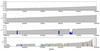 |
Fig. 10 Reachability diagram produced by OPTICS of the unperturbed mean phase-space positions of the 200 000 object sample of Halo-02 with color-coded extracted clusters. |
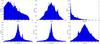 |
Fig. 11 Attribute distributions of the 200 000 stars used to derive the clusterings in test scenario one. |
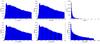 |
Fig. 12 Attribute uncertainty distributions of the 200 000 stars used to derive the clustering in test scenario one. These have been derived using the Gaia science performance specifications and mimic the expected uncertainty distributions of our objects should they be observed by Gaia. |
5.2. Application on a mock stellar halo
We tested FOPTICS’ clustering capabilities and compared its performance with OPTICS using a downscaled sample of Halo-02 containing 200 000 randomly chosen objects within 85 kpc of the galactic center. The downscaling was carried out to limit the computational demands given that the optimizations mentioned in Sect. 3 cannot be applied to FOPTICS. Therefore, its run-time complexity remains at  , where M is the number of samples used to estimate the uncertainty distributions. As a base for comparison, we obtained a clustering of this data set with OPTICS, using the six-dimensional phase-space coordinates. The resulting reachability diagram is shown in Fig. 10. Because of the decreased sample size, the number of detected overdensities is smaller compared to Sect. 4.
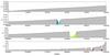 |
Fig. 13 Reachability diagram produced by FOPTICS test case one, in which the data set was perturbed using realistic uncertainties derived from the Gaia science performance specifications. |
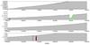 |
Fig. 14 Reachability diagram produced by FOPTICS test case two, in which the data set has been perturbed using five times the uncertainties used in test case one. |
The FOPTICS algorithm requires a number of samples to be drawn from the probability density distributions of the attributes whose clustering is desired. To accommodate this requirement, we created two test scenarios: test scenario (1), which uses Gaia-like uncertainties, and test scenario (2), which uses five times the Gaia-like uncertainties. The uncertainties were derived as follows. Each of our objects has an associated synthetic SDSS u-z luminosity as provided by Robertson et al. (2005), which has enabled the computation of the Gaia white light G and associated end-of-mission parallax error for each of our objects as described in de Bruijne et al. (2005) and Jordi et al. (2010). We derived the expected end-of-mission parallax error σπ given the associated synthetic luminosity. The propagation of σπ through 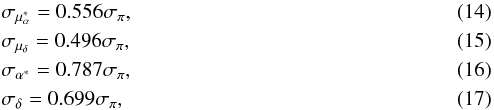 results in the sky position and proper-motion uncertainties. Moreover, the end-of-mission radial velocity uncertainty, σVr, is derived with
 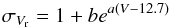 (18)where the a and b coefficients depend heavily on stellar spectral type, as described in de Bruijne (2012). For each of our stars, we assign the spectral type corresponding to the minimum difference between the V−I values shown in Table 1. The uncertainty distributions of each attribute used in test scenario (1) are shown in Fig. 12.
Coefficients used to define a and b in Eq. (18), as described in de Bruijne (2012).
In the first test scenario we created probability densities distributions for each of the attributes (α,δ,π,μα,μδ,Vr) such that each object is described by six normal distributions ( ,
,  ,
,  ,
, 
 ,
,  ). In test scenario two, we increased the Gaia uncertainties by fivefold such that each attribute distribution is described by
  , where X is the unperturbed attribute (used to produce the Fig. 10) and σX is the corresponding Gaia uncertainty (used in the first test scenario) derived in Eqs. (14)–(18). In doing so, any given object covers a larger volume in the multi-dimensional space, which causes their reachability distances to increase and increases the overlap between clusters.
For each of these two test case scenarios, we created 500 distinct samples, where each attribute was drawn from the specified probability density distributions. To avoid discontinuities at α = 0 and 2π [rad] and δ = −π and π [rad] when computing Euclidean distances, the attributes were converted to Cartesian phase-space coordinates, on which the clustering is performed. The reachability diagrams produced by FOPTICS in test scenario one, with Gaia-like uncertainties, and in test scenario two, with five times the Gaia-like uncertainties are shown in Figs. 13 and 14, respectively.
In Figs. 11 and 12 it is clear that a large fraction of the stars used here are extremely faint as defined by their synthetic SDSS u−z luminosities. In these cases, Gaia would not be able to accurately determine both the radial velocity and distance, resulting in high σvr and σR values. We see some vrad values with a relative uncertainty of 1000% and some distance R values with a relative uncertainty of 100%. While these large uncertainties hampers the detection of clusters at large distances, we chose to include them to assess how the FOPTICS handles them.
Comparing the results of OPTICS on the unperturbed phase-space positions (Fig. 10) and the results of FOPTICS (Figs. 13 and 14), it becomes obvious that distinct differences occur when using OPTICS versus FOPTICS, despite the algorithms similiarities. These differences are further distinguished in Fig. 15, where we show the X-R projection of each of the three cases, color coded using the same extracted cluster labels as Figs. 10–14. Particularly, it becomes clear that FOPTICS provides more robust results than OPTICS, such that
-
Size of clusters are more conservative: application of FOPTICS effectively results in the detection of only the most significant portions of clusters, whose densities are sufficiently higher to overcome the effect of uncertainties. Objects with high uncertainties cover a greater extent in multiple dimensions and therefore have higher average reachability distances. As a result, when applying OPTICS the total size of a cluster is overestimated when compared to the results of FOPTICS. These results are clearly visualized in Fig. 16.
-
Streams are shorter and/or unrecognizable: since the inclusion of uncertainties increases the effective volume covered by clusters, objects that make up sparse regions of the streams are diffused into the background, resulting in shorter detected streams, as can be seen in Fig. 16. In extreme cases, where the density of streams is low in comparison to the background the inclusion of uncertainties results in complete non-detection, since the ε-neighborhood condition is not fulfilled.
-
Far clusters are unrecognizable: since Gaia uncertainties are dependent on magnitude and parallax, far and/or faint clusters have high uncertainties. Following the same reasoning as above, these clusters are more likely to be completely diffused into the background owing to the inclusions of their uncertainties.
It is also important to note that in the middle panel and right-hand panel of Fig. 15 one can see by eye several overdensities that were not identified by FOPTICS as genuine clusters. There are several reasons for this. First, a group of stars that show up as an overdensity in a 2D projection can have such large uncertainties that the cluster as a whole rarely survives when its members are perturbed within their error bars. In such case FOPTICS, simply does not detect the overdensity. Secondly, Fig. 15 shows a 2D projection of geometrical coordinates which, despite their uncertainties, are still reasonably localized. The uncertainties in velocity and distance are much larger, especially for the distant clusters, which makes the cluster no longer distinguishable from the diffuse background.
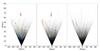 |
Fig. 15 X vs. galactocentric distance projections of a subset of the Halo-02 sample for the unperturbed sample clustered with OPTICS (left), one of the perturbed samples with Gaia-like uncertainties clustered with FOPTICS (middle), and one of the perturbed sampled with five times the Gaia uncertainties also clustered with FOPTICS (right). The extracted clusters in each case were color coded to match their respective reachability diagrams (Figs. 10, 13 and 14, respectively). |
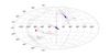 |
Fig. 16 Clusters extracted by OPTICS using the unperturbed mean phase-space positions are shown in black; In red the clusters extracted by FOPTICS using realistic Gaia uncertainities (test case scenario one) and the clusters extracted by FOPTICS using five times the Gaia errors (test case scenario two) in blue. It can be seen that the two streams detected in the data set (blue), using five times that Gaia errors, only the densest portion of the stream were detected with a decreased number points in the tails and therefore a decrease in size. Furthermore, the stream at approximately –15 deg is completely lost when the uncertainties are increased. |
As a side note, we also mention that the processing order of FOPTICS depends on the uncertainty distributions. Since the processing order depends on the minimum averaged dr which is always calculated based on the previously processed point, the order of no two FOPTICS produced reachability diagrams are required to be identical, unless all  data sets are identical. This implies that even two sets of data sets sampled from the same uncertainty distributions can result in slight variations in the order of their fuzzy reachability diagrams. This, however, does not influence the detectability of clusters.
6. Conclusions
In this paper, we presented for the first time an assessment of the performance of a density-based hierarchical clustering algorithm referred to as Ordering Points To Identify the Clustering Structure (OPTICS) on the stellar halo. To obtain the clustering clusters of any multi-dimensional data set, OPTICS linearly orders points, such that any points that are closest in the multi-dimensional space are consecutively sorted. The distance between each point and the previous point is stored and referred to as the reachability distance. The ordered output of the reachability distances is referred to as a reachability diagram, which is a global visualization of the clustering structure of the data set in question. Points that belong to a cluster always have a small reachability distance, and therefore form valleys within the reachability diagram, while points that belong to the background and indicate transitions between clusters have relatively high reachability distances, and form peaks.
A few parameters control OPTICS clustering and performance: the minimum cluster size Nmin; Tmin, which describes the minimum acceptable reachability distance of transitions peaks; and the similarity ratio Ts, which describes the acceptable similarity of an overdensity that can stand-alone or is a substructure of a larger overdensity. The use of these parameters enables the user to finetune the algorithm for varying scientific purposes. For our purpose, we chose parameters that enable an appropriate balance between completeness and contamination of the resulting halo structures. If one is only interested in large-scale structures, high values of all three parameters should be used, while if one is mainly interested in the substructure of larger structures lower values of Nmin and Tmin are recommended.
In our application on a realistic mock stellar halo, we have shown that OPTICS is capable of detecting large- and small-scale structures and substructures, making it a viable algorithm for the detection of overdensities in the stellar halo. Moreover, we obtained low cluster contamination values showing that the method can be configured to be conservative. Additionally, the reachability diagram has proven to be a very convenient tool to easily grasp the size, density, and density variations within a cluster. We proposed the Jaccard index to investigate the cluster stability. As a proxy to cluster significance this index, computed using bootstrapping the original sample, avoids the need to estimate the local background density first and becomes particularly convenient in the case of large extended overdensities that are embedded in a varying background.
In the process of showing OPTICS viability, we implemented several optimization techniques that make the algorithm computationally inexpensive without the need for parallelization. Even without parallellization, we were able to successfully cluster samples of up to 8 million stars in six-dimensional phase-space in approximately 12 min on a single CPU, and we obtained a slightly super-linear run-time complexity, making it a compelling algorithm for large data sets such as the data set obtained with Gaia.
Additionally, OPTICS can be generalized into a unique algorithm called Fuzzy Ordering Points To Identify the Clustering Structure (FOPTICS), which enables the incorporation of attribute uncertainty during the clustering. At the heart of the algorithm is a Monte Carlo approach where the attributes of the stars are resampled within their uncertainty ellipsoids and clustered independently in a similar way as for OPTICS; the main difference is how the algorithm determines the nearest consecutive point. The method that FOPTICS uses to aggregate the results of these repeated applications into one comprehensive final clustering result turns out to work very well. Groups of close stars with large uncertainty ellipsoids in phase space are no longer detected as significant clusters unless the cluster size and density is sufficiently large to overcome the effect of the attribute uncertainty distributions. Furthermore, we find that the sizes and extent of detected clusters and tidal streams are more conservative, as the far part usually has larger uncertainties than the nearby part.
A disadvantage of FOPTICS is that the optimizations used to accelerate OPTICS cannot be applied. In the case of OPTICS, the neighborhood queries were sped up to avoid the worse-case  complexity. When the uncertainty ellipsoids of the stars are taken into account, however, there is always a non-zero probability for any two stars in the sample to be closest neighbors. Hence few optimizations can be implemented, making it difficult to improve upon the complexity of the nearest neighbors search. As described in Sect. 5.2, one FOPTICS run where overdensities were searched in a sample of 200 000 stars in a 6D phase space with uncertainty ellipsoids, took roughly 100 CPU hours. An application to millions of stars is therefore still within reach, provided that the computations can be performed on a grid computer or additional optimizations are implemented.
Acknowledgments
S.A.S.F. acknowledges support of the KU Leuven contract GOA/13/012. The authors would like to thank Amy X. Zhang at MIT CSAIL for providing a skeleton version of the Sander et al. (2003) extraction method which has been modified for our purposes. The authors would like to thank the anonymous referee for useful comments that have improved this article.
References
- Ankerst, M., Breunig, M. M., peter Kriegel, H., & Sander, J. 1999, in Optics: Ordering points to identify the clustering structure (ACM Press), 49 [Google Scholar]
- Behroozi, P. S., Wechsler, R. H., & Conroy, C. 2013, ApJ, 770, 57 [NASA ADS] [CrossRef] [Google Scholar]
- Bullock, J. S., & Johnston, K. V. 2005, ApJ, 635, 931 [NASA ADS] [CrossRef] [Google Scholar]
- Bullock, J. S., Kravtsov, A. V., & Weinberg, D. H. 2001, ApJ, 548, 33 [NASA ADS] [CrossRef] [Google Scholar]
- de Bruijne, J. 2012, Astrophys. Space Sci., 341, 31 [Google Scholar]
- de Bruijne, J., Perryman, M., Lindegren, L., et al. 2005, Gaia astrometic, photometirc, and radial velocity performance assessment methodologies to be used by the industrial system-level teams, Tech. Rep. (European Space Agency) [Google Scholar]
- Diemand, J., Kuhlen, M., & Madau, P. 2006, ApJ, 649, 1 [NASA ADS] [CrossRef] [Google Scholar]
- Elahi, P. J., Han, J., Lux, H., et al. 2013, MNRAS, 433, 1537 [NASA ADS] [CrossRef] [Google Scholar]
- Font, A. S., Johnston, K. V., Bullock, J. S., & Robertson, B. E. 2006a, ApJ, 638, 585 [Google Scholar]
- Font, A. S., Johnston, K. V., Bullock, J. S., & Robertson, B. E. 2006b, ApJ, 646, 886 [NASA ADS] [CrossRef] [Google Scholar]
- Helmi, A. 2008, A&ARv, 15, 145 [CrossRef] [Google Scholar]
- Hennig, C. 2007, Comput. Statist. Data Analysis, 52, 258 [CrossRef] [Google Scholar]
- Hofmans, J., Ceulemans, E., Steinley, D., & Van Mechelen, I. 2015, J. Classification, 32, 268 [CrossRef] [Google Scholar]
- Ibata, R. A., Gilmore, G., & Irwin, M. J. 1994, Nature, 370, 194 [NASA ADS] [CrossRef] [Google Scholar]
- Ivezić, Ž., Monet, D. G., Bond, N., et al. 2008, in A Giant Step: from Milli- to Micro-arcsecond Astrometry, eds. W. J. Jin, I. Platais, & M. A. C. Perryman, IAU Symp., 248, 537 [Google Scholar]
- Johnston, K. V., Hernquist, L., & Bolte, M. 1996, ApJ, 465, 278 [NASA ADS] [CrossRef] [Google Scholar]
- Jordi, C., Gebran, M., Carrasco, J. M., et al. 2010, A&A, 523, A48 [NASA ADS] [CrossRef] [EDP Sciences] [Google Scholar]
- Keller, S. C., Schmidt, B. P., Bessell, M. S., et al. 2007, PASA, 24, 1 [NASA ADS] [CrossRef] [Google Scholar]
- Knebe, A., Knollmann, S. R., Muldrew, S. I., et al. 2011, MNRAS, 415, 2293 [NASA ADS] [CrossRef] [Google Scholar]
- Kriegel, H., & Pfeifle, M. 2005, in Proc. Eleventh ACM SIGKDD International Conference on Knowledge Discovery and Data Mining, Chicago, Illinois, USA, August 21–24, 672 [Google Scholar]
- Maciejewski, M., Colombi, S., Springel, V., Alard, C., & Bouchet, F. R. 2009, MNRAS, 396, 1329 [NASA ADS] [CrossRef] [Google Scholar]
- Mucha, H.-J., Bartel, H.-G., e. L. B., Krolak-Schwerdt, S., & Bøhmer, M. 2015, Resampling Techniques in Cluster Analysis: Is Subsampling Better Than Bootstrapping? (Berlin, Heidelberg: Springer Berlin Heidelberg), 113 [Google Scholar]
- Perryman, M. A. C. 2002, Ap&SS, 280, 1 [Google Scholar]
- Pfitzner, D. W., Salmon, J. K., & Sterling, T. 1997, Data Mining and Knowledge Discovery, 1, 419 [CrossRef] [Google Scholar]
- Robertson, B., Bullock, J. S., Font, A. S., Johnston, K. V., & Hernquist, L. 2005, ApJ, 632, 872 [NASA ADS] [CrossRef] [Google Scholar]
- Sander, J. o., Qin, X., Lu, Z., Niu, N., & Kovarsky, A. 2003, in Proc. 7th Pacific-Asia Conference on Advances in Knowledge Discovery and Data Mining, PAKDD ’03 (Berlin, Heidelberg: Springer-Verlag), 75 [Google Scholar]
- Sharma, S., & Johnston, K. V. 2009, ApJ, 703, 1061 [NASA ADS] [CrossRef] [Google Scholar]
- Springel, V., White, S. D. M., Tormen, G., & Kauffmann, G. 2001, MNRAS, 328, 726 [Google Scholar]
All Tables
Coefficients used to define a and b in Eq. (18), as described in de Bruijne (2012).
All Figures
|
Fig. 1 Top panel: two-dimensional cluster distribution used to produce the reachability diagram below. Bottom panel: associated reachability diagram, order vs. the normalized reachability distance Dr, resulting from applying OPTICS to the above data set. The color coding and arrows indicate the location of each cluster within the reachability diagram. |
| In the text | |
|
Fig. 2 Run time complexity of our implementation of OPTICS shown in Log-Log scales. The red line indicates the linear least-squares fit, whose slope is 1.16, indicating a near linear complexity. |
| In the text | |
|
Fig. 3 Aitoff projection of all 483 733 objects, composing a total of 74 unique clusters, used to cluster Halo-02. |
| In the text | |
|
Fig. 4 Top panel: reachability diagram produced by OPTICS when clustering the down-scaled Halo-02 sample. As per definition, the x-axis represents the processing order derived from OPTICS and the y-axis gives the normalized reachability (Dr) where dr has been normalized to the highest defined value and all undefined values set to one. Bottom panel: Aitoff projection of objects used in the clustering of Halo-02. Each extracted cluster was color coded to show its location in both the reachability diagram and the Aitoff projection. Comparing Fig. 3 and the Aitoff projection presented here it is clear that OPTICS recovers all of the clusters that are visible by eye. More importantly, OPTICS is able to disentangle clusters that appear to overlap in their Aitoff projections. |
| In the text | |
|
Fig. 5 X-Y projections of Bullock & Johnston (2005) overdensity 63 (left) and overdensity 33 (right) are plotted in black. The OPTICS partitions are overplotted in red. The other overlapping overdensities are not plotted for the sake of clarity, but are the main reason the completeness is not 100%. |
| In the text | |
|
Fig. 6 Identification numbers of the clusters CO detected by OPTICS vs. the identification numbers of the true clusters CT with the largest overlap. Sometimes a true cluster is detected by OPTICS as multiple clusters. This simply indicates that the chain of ε-neighborhoods connecting two or more sections of the same cluster has been broken due to poorly connected parts or because a part was assigned to another strongly overlapping cluster. |
| In the text | |
|
Fig. 7 Left-hand panel: completeness of each cluster CO extracted by OPTICS with respect to the original cluster CT given by Bullock & Johnston (2005). The low values are because many streams experienced a tidal breakup, and the individual partitions detected by OPTICS were compared with the entire stream size. Right-hand panel: what fraction of true clusters show up in any cluster extracted by OPTICS. Many overdensities are recovered with a large total completeness. Some of the low total completeness values come from clusters that are so sparse compared to the background that they are difficult to distinguish. The middle panel shows the contamination in each cluster extracted by OPTICS. |
| In the text | |
|
Fig. 8 Left-hand panel: histogram of the completeness the OPTICS extracted cluster (CO). It is clear that a large fraction of our detected clusters have low completeness values, as explain in the caption of Fig. 7 and in the text. Middle panel: contamination histogram, where it is obvious that the vast majority of our detected clusters have contamination rates of less than 10%. Right-hand panel: histogram of what fraction of true clusters show up in any cluster extracted by OPTICS. A dichotomy is can be seen in this panel, where clusters are either very well recovered or only a small fraction are detected. The low total completeness values come from clusters that are so sparse compared to the background that they are difficult to distinguish. |
| In the text | |
|
Fig. 9 Stability index for each of the extracted clusters in the original sample. The black line indicates a cutoff limit of 0.5. 63 Clusters are above this cutoff limit that can be considered significant and stable. |
| In the text | |
|
Fig. 10 Reachability diagram produced by OPTICS of the unperturbed mean phase-space positions of the 200 000 object sample of Halo-02 with color-coded extracted clusters. |
| In the text | |
|
Fig. 11 Attribute distributions of the 200 000 stars used to derive the clusterings in test scenario one. |
| In the text | |
|
Fig. 12 Attribute uncertainty distributions of the 200 000 stars used to derive the clustering in test scenario one. These have been derived using the Gaia science performance specifications and mimic the expected uncertainty distributions of our objects should they be observed by Gaia. |
| In the text | |
|
Fig. 13 Reachability diagram produced by FOPTICS test case one, in which the data set was perturbed using realistic uncertainties derived from the Gaia science performance specifications. |
| In the text | |
|
Fig. 14 Reachability diagram produced by FOPTICS test case two, in which the data set has been perturbed using five times the uncertainties used in test case one. |
| In the text | |
|
Fig. 15 X vs. galactocentric distance projections of a subset of the Halo-02 sample for the unperturbed sample clustered with OPTICS (left), one of the perturbed samples with Gaia-like uncertainties clustered with FOPTICS (middle), and one of the perturbed sampled with five times the Gaia uncertainties also clustered with FOPTICS (right). The extracted clusters in each case were color coded to match their respective reachability diagrams (Figs. 10, 13 and 14, respectively). |
| In the text | |
|
Fig. 16 Clusters extracted by OPTICS using the unperturbed mean phase-space positions are shown in black; In red the clusters extracted by FOPTICS using realistic Gaia uncertainities (test case scenario one) and the clusters extracted by FOPTICS using five times the Gaia errors (test case scenario two) in blue. It can be seen that the two streams detected in the data set (blue), using five times that Gaia errors, only the densest portion of the stream were detected with a decreased number points in the tails and therefore a decrease in size. Furthermore, the stream at approximately –15 deg is completely lost when the uncertainties are increased. |
| In the text | |
Current usage metrics show cumulative count of Article Views (full-text article views including HTML views, PDF and ePub downloads, according to the available data) and Abstracts Views on Vision4Press platform.
Data correspond to usage on the plateform after 2015. The current usage metrics is available 48-96 hours after online publication and is updated daily on week days.
Initial download of the metrics may take a while.