| Issue |
A&A
Volume 692, December 2024
|
|
|---|---|---|
| Article Number | A194 | |
| Number of page(s) | 12 | |
| Section | Galactic structure, stellar clusters and populations | |
| DOI | https://doi.org/10.1051/0004-6361/202451078 | |
| Published online | 13 December 2024 | |
Obscured star clusters in the inner Milky Way
How many massive young clusters are still awaiting detection
1
Universitäts-Sternwarte, Fakultät für Physik, Ludwig-Maximilians-Universität München,
Scheinerstr. 1,
81679
München,
Germany
2
European Southern Observatory,
Karl-Schwarzschild-Str. 2,
85748
Garching bei München,
Germany
3
Instituto de Astrofísica, Depto. de Ciencias Físicas, Facultad de Ciencias Exactas, Universidad Andrés Bello,
Av. Fernandez Concha 700, Las Condes,
Santiago,
Chile
4
Vatican Observatory,
Vatican City State,
V-00120,
Italy
★ Corresponding authors; agupta@ph1.uni-koeln.de, preibisch@usm.uni-muenchen.de, vivanov@eso.org
Received:
12
June
2024
Accepted:
1
November
2024
Context. Milky Way star clusters provide important clues about the history of star formation in our Galaxy. However, the dust in the disk and in the innermost regions hides them from the observers.
Aims. Our goal is twofold. First, to detect new clusters – we have applied the newest methods of detecting clusters with the best available wide-field sky surveys in the mid-infrared because they are the least affected by extinction. Second, we address the question of cluster detection’s completeness, for now limiting it to the most massive star clusters.
Methods. This search is based on the mid-infrared Galactic Legacy Infrared Mid-Plane Survey Extraordinaire (GLIMPSE), to minimize the effect of dust extinction. The search Ordering Points To Identify the Clustering Structure (OPTICS) clustering algorithm was applied to identify clusters, after excluding the bluest, presumably foreground sources, to improve the cluster-to-field contrast. The success rate for cluster identification was estimated with a semi-empirical simulation that adds clusters, based on the real objects, to the point source catalog, to be recovered later with the same search algorithm that was used in the search for new cluster candidates. As a first step, this was limited to the most massive star clusters with a total mass of ~104 M⊙.
Results. Our automated search, combined with inspection of the color-magnitude diagrams and images, yielded 659 cluster candidates; 106 of these appear to have been previously identified, suggesting that a large hidden population of star clusters still exists in the inner Milky Way. However, the search for the simulated supermassive clusters achieves a recovery rate of 70–95%, depending on the distance and extinction toward them.
Conclusions. The new candidates – if confirmed – indicate that the Milky Way still harbors a sizeable population of unknown clusters. However, they must be objects of modest richness, because our simulation indicates that there is no substantial hidden population of supermassive clusters in the central region of our Galaxy.
Key words: Galaxy: disk / open clusters and associations: general / Galaxy: stellar content / Galaxy: structure
© The Authors 2024
 Open Access article, published by EDP Sciences, under the terms of the Creative Commons Attribution License (https://creativecommons.org/licenses/by/4.0), which permits unrestricted use, distribution, and reproduction in any medium, provided the original work is properly cited.
This article is published in open access under the Subscribe to Open model. Subscribe to A&A to support open access publication.
1 Introduction
Stars are the basic building blocks of galaxies and the vast majority of them form in a clustered environment (Lada & Lada 2003). Hence, a complete census of star clusters in the Milky Way is important for tracing star formation, chemical enrichment, and galactic structure – studies of young massive clusters have an impact on many areas (Portegies Zwart et al. 2010). A major obstacle to finding star clusters is the extinction that light suffers due to the dust along the line of sight and this becomes even more severe when the clusters are located closely within the disk of our Galaxy. Optical surveys like HIPPARCOS and Gaia have been successful in cataloging the clusters in the solar neighborhood (see for example Platais et al. 1998; Koposov et al. 2017) but the star clusters farther away – and behind more dust – become undetectable in optical surveys.
Infrared (IR) surveys allow us to find star clusters close to the Galactic center, like the massive Arches cluster (Nagata et al. 1993, 1995), and to address the question how close to the center of the Milky Way the clusters can survive (Minniti et al. 2021a). Since then, there have been a lot of dedicated IR cluster searches. In a major effort, Dutra & Bica (2001) visually inspected 2MASS (Two Micron All Sky Survey; Skrutskie et al. 2006) images searching for clusters in the Cygnus X region. A wider automated search covering 47% of the sky in the 2MASS point source catalog was carried out by Ivanov et al. (2002); new clusters were detected using as apparent stellar surface density peaks and then verified with a visual inspection to avoid artifacts caused by, for example, dust clouds. Further productive near-IR star cluster searches have been carried out with the UKIDSS and VVV/VVVX surveys (Borissova et al. 2011; Minniti et al. 2011, 2021b; Solin et al. 2012; Barbá et al. 2015; Borissova et al. 2018).
However, the near-IR cluster census is also subjected to incompleteness, as was shown by Ivanov et al. (2005, see their Figure 7), because the extinction in the inner Milky Way can be considerable even at these wavelengths (e.g., AKS ~2.8 mag corresponding to AV~ 30 mag to some clusters; Kurtev et al. 2008). One way to overcome this challenge is to turn toward mid-IR wavelengths and surveys like GLIMPSE (Galactic Legacy Infrared Mid-Plane Survey Extraordinaire; Benjamin et al. 2003) and WISE (Wide Infrared Survey Explorer; Wright et al. 2010).
Along these lines, Mercer et al. (2005) used 2D Gaussian fitting to the surface density of sources in the GLIMPSE point source catalog to identify potential clusters and estimate their locations and sizes. They removed false positives with statistical significance tests, finding 59 new, mostly highly embedded clusters. Importantly, as we shall discuss further, no constraints on the stellar colors were imposed. Morales et al. (2013) pointed out that this approach would more likely identify nearby bright sources and would still miss, despite working in the mid-IR regimen, many of the reddened clusters because of the mix of sources at different distances along the line of sight and the ensuing confusion. To counter this, Morales et al. (2013) only considered red sources with GLIMPSE color [4.5]−[8.0]≥;1 mag. In this work, no photometric quality constraints were applied, which strongly affected the contribution from faint stars. Still, their simple automated algorithm yielded 75 new clusters, most of them embedded. Finally, Ryu & Lee (2018) identified 923 cluster candidates with a visual search in WISE, but the vast majority of them have not been validated, even through a simple inspection of the color-magnitude diagrams (CMDs). Camargo et al. (2016) identified 652 stellar clusters close to the galactic plane (mostly embedded) using a radial density profile (RDP), and CMDs in WISE data raise a good question about how many more clusters are present in the disk.
The Milky Way cluster census remains incomplete, despite the move toward the longer wavelengths and multiple efforts by various teams. In particular, the region close to the Galactic center, accessible only through IR observations, is especially interesting because of the number of candidate star clusters that still need confirmation and determination of physical parameters. In this work, we pursue two goals, with corresponding improvements. First, we want to address, albeit for now in a limited way, the long-neglected question of how complete the existing cluster catalogs are. Adding tens or thousands of new clusters means little if we do not know whether this number of objects amounts to 1 or 50 or 99% of the entire Milky Way cluster population. Some early simulation efforts were carried out by Ivanov et al. (2010) and Hanson et al. (2010), who generated a galaxy-wide cluster population immersed in dust. Both the cluster and the dust followed smooth exponential spatial distributions. The model calculated the line-of-sight extinction to individual clusters and their visibility, estimating what fraction of the Milky Way clusters are visible. Mercer et al. (2005) introduced artificial clusters with Gaussian profiles in the GLIMPSE point source catalog and they reported that all the artificial clusters were detected by their search algorithm. Recently, Nambiar et al. (2019) simulated the cluster detection efficiency of the Parzen density estimation method but did not tie the results to a particular survey or type of cluster. Parzen density estimation, also referred to as Parzen windows or kernel density estimation, is a nonparametric method used in statistics to estimate the probability density function of a random variable based on a finite sample of data points (Parzen 1962).
The most robust way of estimating the detection rate is to carry out a controlled experiment by adding a sample of simulated star clusters. In the most general case, the simulated clusters must span the full range of cluster parameters – most importantly, masses and ages. Another necessary component of such a simulation is a detailed 3D extinction map of our Galaxy.
Simulating the entire Milky Way cluster population and measuring the detection rates for different classes of clusters is difficult and here, in this pilot study, we have only considered the case of the most massive clusters, analogous to Westerlund 2 (Westerlund 1961b). It is located relatively nearby at 4.16±0.33 kpc from us and has an age of 1–2 Myr (Zeidler et al. 2015). It was adopted as an empirical template because it falls within the GLIMPSE footprint and a recent photometric estimate of (3.7±0.8)×104 M⊙ (Zeidler et al. 2021) places it among the most massive Milky Way clusters. Only a handful of similar objects are known: Arches (Nagata et al. 1993, 1995), RSGC 1 (Bica et al. 2003; Davies et al. 2007), the Galactic Center Cluster (Becklin & Neugebauer 1968), Quintuplet (Okuda et al. 1990; Nagata et al. 1990), and Westerlund 1 (Westerlund 1961a; Moffat et al. 1991). Although rare, they are important as examples of galactic building blocks and they are local (mini-)analogs of distant star-forming galaxies (Portegies Zwart et al. 2010).
Finding more massive clusters is challenging, especially in the relatively narrow age range when the total cluster luminosity in the IR – where they emit most of their light – is dominated by pre-main-sequence stars, while the rest of the stars are significantly fainter in the IR. This makes the question of whether the Milky Way contains more of them particularly relevant.
Our other aim is to complete the Milky Way cluster census further, while taking advantage of the new and improved search algorithms, finding undiscovered and highly obscured clusters. The new generation of algorithms is based on machine learning (ML). To increase our chances of cluster identification, we considered only sources with reliable [3.6] and [4.5] GLIMPSE photometry (errors ≤0.2 mag) and only the red stars of [3.6]−[4.5]>0.6 mag (see Sect. 2.2.2). This limit is different than that of Morales et al. (2013, [4.5]−[8.0]>1.0 mag), who set theirs after Robitaille et al. (2008). Our color limit is more sensitive to the stars’ emission than to the dust because it omits the [8.0] band, and therefore it better removes the stellar foreground contamination. We underline that our search is optimized for the detection of distant and highly reddened clusters – the type that is likely to suffer the worst incompleteness.
Our two goals are intertwined because the completeness analysis requires having to hand a reliable cluster detection tool. Staying on the side of caution, we consider the identified clusters to be candidates, because in all fairness we cannot exclude false positives, related to dust clouds and spurious stellar density variation that can exhibit cluster-like morphology. Deep IR astrometry or time-consuming follow-up spectroscopy, also in the IR, is needed to confirm the cluster nature of the candidates.
The next section presents the GLIMPSE data, the new clustering algorithm, and the properties of the newly found candidates. The artificial cluster simulation is described in Sect. 3, and Sect. 4 summarizes our results.
2 Cluster search
2.1 The GLIMPSE survey
We have used the GLIMPSE catalog from Spitzer Science (2009), which combines GLIMPSE-I v2.0, GLIMPSE-II v2.0, and GLIMPSE-3D. The catalog is available at CDS1 and includes:
GLIMPSE-I (Benjamin et al. 2003), covering the area of |l|=10-65° and |b|≤1°, and the Observation Validation Strategy region around l=240°.
GLIMPSE-II (Spitzer Science 2009), covering the regions of: |l|<2° and |b|≤2°, |l|=2–5° and |b|≤1.5°, and |l|=5–10° and |b|≤1°. It omits the Galactic center region at |l|≤1°, |b|≤0.75°, but data for this region from the General Observer program, GALCEN (PID=3677, PI Stolovy), is included.
GLIMPSE-3D (Spitzer Science 2009) adds vertical extension stripes of up to |b|<4.2° at the center of the Galaxy and up to |b|<3° elsewhere.
These catalogs overlap in some regions, and in such cases the order of priority is GLIMPSE-II, GLIMPSE-I, and GLIMPSE-3D, as is described in the documentation on the GLIMPSE website2. The catalog was cross-matched with various other surveys like 2MASS, with a matching radius of 0.1″, testifying to the excellent astrometric calibration of this survey.
2.2 Search method
2.2.1 OPTICS clustering algorithm
Ordering Points To Identify the Clustering Structure Clustering algorithm (OPTICS; Ankerst et al. 1999) is a density-based clustering algorithm, a further development of Density-Based Spatial Clustering of Applications with Noise (DBSCAN; Ester et al. 1996). Unlike DBSCAN, which combines the objects into clusters, OPTICS orders by their reachability-distance to the closest core object from which they have been directly density-reachable.
Here, a core object is an object that can be reached by at least as many objects, as the required minimal number of members (min_samples) that groups should contain in order to be considered a cluster. A cluster grows until the reachability-distance to the next potential member exceeds some limit – the maximum distance between two stars within which they will be considered reachable or members of the same cluster (hereafter, eps, measured in degrees). The effect these parameters have on the results will be discussed in Sect. 2.2.2.
The method allows for a hierarchy of clusters and, given the nature of the star formation that tends to occur in structures of different sizes, from giant star-forming regions to compact star clusters, we consider it important to preserve this hierarchy. Admittedly, here we do not take full advantage of its power, optimizing the search parameters to identify distant and relatively compact clusters, but this is an important feature if one aims at the nearer clusters that are embedded in large star-forming regions.
2.2.2 Data curation and search parameters
It proved unpractical to run the cluster search over the entire GLIMPSE footprint, because of the memory and speed requirements to handle the entire catalog. Therefore, we fragmented it into 1°×1° tiles for easier data handling. This size was a compromise between computational requirements and the danger of missing clusters that are split between two neighboring tiles on the other side. For a typical cluster diameter of ~1′, the probability that a cluster would be split between two tiles is ~3%, and we ignored these cases.
Next, to ensure good-quality data, we considered only GLIMPSE sources with photometric errors of <0.2 mag in both bands, [3.6] and [4.5]. This requirement affects the faint end of the apparent luminosity function below [3.6]≥15.5 mag where the color becomes so uncertain that it is impossible to discriminate between a typical foreground lower main-sequence star and a highly reddened distant cluster member star at a level better than 3–5 σ. We also set an upper color limit of [3.6]−[4.5]=4 mag, because upon inspection most of reddest sources appear to be galaxies. This is not the case for the innermost regions of the Milky Way, but our experiments indicate that the surface density of these sources is typically too low to meet the minimum number of cluster members that we require. Therefore, this limit can probably be ignored in further searches. Furthermore, we have no strict way to confirm the membership of individual objects in a cluster; therefore, the members are actually suspected or candidate members.
Last but not least, we applied color criteria as a proxy for the reddening and for the distance to individual stars, assuming the reddening and the distance are proportional, to zero order. Running the search on each color bin separately minimizes the field star contamination and improves the cluster-to-field contrast. The extinction and distance are not linearly related and the clumpy structure of the dust makes this relation even more complex. The existing extinction maps, even the 3D ones, are of little help because they are based on the red clump stars that probe the reddening via older populations. An accurate 3 D reddening map suitable to remove the reddening toward younger clusters will not be available until an IR analog of Gaia becomes available.
To investigate the effect of the color binning, we split the GLIMPSE sources into multiple [3.6]−[4.5] color bins: [0.0, 0.2], [0.2, 0.4], [0.4, 0.6], and [0.6, 4], and ran the search on each of them separately with the same parameters: requiring a minimum of 12 member stars per cluster candidate (following classical definitions from: Portegies Zwart et al. 2010; Trumpler 1930) and a maximum radius of the candidate of 6′. Table 1 shows the number of candidates for the different bins. It is lower toward redder bins and many candidates were detected in more than one bin: 10094 appear in both the first two bins, 944 in the first three, and 66 in all four bins. A random inspection suggested that a large fraction of candidates are spurious, especially in the most populated bluer bins. The cluster-to-field contrast increases toward redder bins, because of the omitted foreground population, but on the other hand the reddest bins are sparsely populated, and searching in them alone would leave too many clusters undetected. In the end, we adopted a single color bin of [0.6, 4] as a compromise between two goals: to ensure that we identify the reddest and most obscured candidates and to exclude the vast blue foreground stellar population.
We investigated how the OPTICS parameters eps min_samples affect the candidate yield using a 15°<l<35° GLIMPSE cutout. SIMBAD lists 99 bona fide star clusters in this area. We considered five parameter combinations: (min_samples, eps): (30, 6′), (30, 6′), (12, 3′), (12, 1′), and (12, 6′). These values were selected to span the typical cluster sizes and richness of known obscured clusters. Our success metric was the fraction of recovered known clusters. The results are listed in Table 2, and the distribution of the candidate cluster sizes are shown in Fig. 1.
This low recovery rate is a concern and we investigated why so many known clusters remained undetected. One reason was that many of them were nearby, subjected to little or negligible reddening, and were excluded by our color criterion. Indeed, of the 55 undetected clusters, 15 were identified from Gaia observations, 11 are classified in SIMBAD as stellar associations, and 2 are nearby and NGC clusters, many of which consist of young blue stars. This brings our failure rate from ~44% down ~27% – still high and calling for further investigation in a forthcoming paper.
A larger eps and a smaller min_samples increase the number of identified candidates; a smaller eps and a large min_samples tend to detect more compact candidates, missing sparser clusters. Notably, the first two parameter combinations yield few candidates and a significantly lower fraction of recovered clusters than the other three combinations and these candidates have bigger sizes. Therefore, these two combinations are better for finding bigger and presumably closer clusters, which fall outside of the goal of this work to identify distant and heavily obscured clusters, because these types of clusters would be readily detected in optical searches, including with Gaia.
The last three parameter combinations require a lower number of member stars (12) and a range of minimum radius (6′, 3′, and 1′). The first two of these yield very similar results. Remembering our goal, we adopted the (12, 6′) parameter combination as a compromise – to be sensitive to compact clusters but also to make our detection more complete. Of course, we accept the risk of contamination in our findings with relatively nearby and sparse clusters.
Counterintuitively, clusters can have radii greater than the maximum distance between two stars eps, especially in regions of high source density. The eps defines the maximum distance between density-reachable points that are considered neighbors. The algorithm can build a sequence of neighbors where the ultimate points are further apart than eps but are connected with regions of higher density. The concept of clusters in OPTICS is broader and the size and shape of clusters trace the density distribution of the data. Therefore, clusters in OPTICS may span distances greater than the adopted maximum distance.
In the software implementation of this and the following steps, we widely used the basic Python modules, AstroPy and Matplotlib (Astropy Collaboration 2018, 2022; Hunter 2007).
Number of clusters (Nclusters) detected in various bins.
Performance of the algorithm on various parameters.
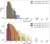 |
Fig. 1 Distribution of candidate cluster sizes for different search parameters. |
2.3 Screening of cluster candidates
Our search with the adopted parameters yielded 10 907 candidates. The experience of previous searches has shown that many, if not most of them, are not real clusters. For example, the clumpy dust distribution leads to artificial “overdensities” around the edges of dark clouds that may significantly exceed the average surface density of the surrounding field, just because the dark cloud prevents us from seeing many background sources. This issue is only partially alleviated by applying color selection criteria, because the color criteria are usually more efficient at removing the foreground than the background. Furthermore, the spatial stellar distribution is uneven itself and can produce enhanced surface density regions – either because of large structures, such as spiral arms viewed along the line of sight (e.g., Kaltcheva & Georgiev 1993), or because of stochastic density peaks (e.g., Asa’d et al. 2023).
In the absence of spectroscopic observations, the sole means to verify the nature of the candidates is an inspection of the CMDs and three-color images from the available mid- and nearIR surveys. The requirement that the CMDs show some of the typical cluster sequences adds in effect a degree of physical – albeit unquantifiable – constraints, in addition to the geometric ones imposed by the overdensity search.
We calculated several parameters for each candidate:
– (l, b): center in the Galactic coordinate system, determined by taking the median averages of longitudes and latitudes of all individual objects grouped by the algorithm.
– nclust_OPTICS: number of stars “assigned” to the cluster by the OPTICS clustering algorithm.
– cluster radius: calculated by taking the mean of the Euclidean distance along l and b from the center of the two farthest candidate member objects (identified by the OPTICS algorithm).
– no. cluster members (Ncluster): number of GLIMPSE objects (with 0.6 mag≤[3.6]−[4.5]≤4.0 mag) that fall inside the candidate area, defined as a circle with a diameter equal to the derived cluster size.
– no. field sources (Nfield): for comparison reasons, we need a sample of foreground and background stars in a nearby locus with the same area as that of the cluster. This field helps us to verify the overdensity and to estimate which parts of the CMD are contaminated by field sources. We obtained such a sample within a circular annulus surrounding the candidate cluster. The inner radius of the “sky” annulus is 30% larger than the cluster radius to avoid problems due to the uncertain cluster size.
– overdensity (σ): excess number of stars in the cluster over the number of stars in the field in units of the background root mean square (assuming Poisson statistics):
![$\[\sigma=\frac{\mathrm{N}_{\text {cluster }}-\mathrm{N}_{\text {field }}}{\sqrt{\mathrm{N}_{\text {field }}}}.\]$](/articles/aa/full_html/2024/12/aa51078-24/aa51078-24-eq1.png) (1)
(1)
For the overdensity calculation, we counted as members all stars within the candidate’s locus and all stars in the field annulus that meet the same color and error criteria adopted for the cluster search. Therefore, the estimated overdensity should be treated with caution because it includes a certain fraction of foreground and background objects.
To facilitate an efficient screening of thousands of candidates, we created a custom at-a-glance visualizer Python tool that combines these numbers and other information we have for each object. The main criteria for the true cluster nature of a candidate were that it has a statistically significant excess of stars near the center, that these stars are more reddened than their surrounding counterparts, and that they cluster in the CMDs in a locus that resembles a reddened main-sequence or red giant branch and show circular symmetry – with some leeway for asymmetries due to differential reddening, for example. We “trained” on benchmark embedded clusters from Morales et al. (2013). Figure 2 shows a CMD inspection image of a known embedded cluster (left) and a candidate from our catalog (right). The candidate has higher overdensity, supporting the clustered nature of this object. This is especially obvious upon inspection of the mid-IR CMD (upper left panels) if one counts the red dots with [3.6]−[4.5]>0.6 mag (marked with dotted vertical lines) and with [3.6] in the range of 8–12 mag and compares their number with the number of black dots in the same locus – here, the red dots mark the stars within the cluster region and black dots are the stars in the comparison field annulus (both regions have the same areas and are marked with red and black circles, respectively, on the right panels). The inspection also included the three-color 2MASS (JHKS bands), WISE (W1, W2, W4 bands), and GLIMPSE ([3.6], [4.5], and [8.0] bands) images of candidates that passed the CMD check. These images for the object in Fig. 2 (left) are shown in Fig. 3. The object is virtually invisible in the near-IR three-color image. This step is important for excluding candidates located next to dense dust clouds that generate a necklace-like chain of clusters.
In summary, these two steps of screening reduced the sample size to 659 candidates, listed in Table 3. It shows the adopted nomenclature for their identification. Their location on the Milky Way map is shown in Fig. 4 (generated with the Python module mw_plot3). Importantly, this inspection of the candidates is a subjective step that relies heavily on human judgment, despite the “training” on the known clusters.
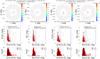 |
Fig. 2 Cluster candidate verification plots for a known recovered cluster (G3CC 8; Morales et al. 2013, left) and for a new candidate (right). The titles list the derived cluster parameters (see Sects. 2.3 and 3 for more details). Panels: Top left – Mid-IR CMD; red dots are all sources within the cluster radius and black dots are all sources in the sky annulus. Top right – Map of GLIMPSE sources with colors in the bin 0.6 mag≤[3.6]−[4.5]≤4.0 mag, color-coded by [3.6]−[4.5]. The red circle shows the cluster region and the black rings the sky annulus. Middle left – Combined near/mid-IR CMD; the dots are coded lines in the panel above. Middle right – Map of GLIMPSE-2MASS sources. Black dots represent all sources, while larger dots color-coded by [K]−[3.6] are the objects with 0.6 mag≤[3.6]−[4.5]≤4.0 mag. Bottom left – Mid-IR [3.6]−[4.5] color histogram for sources in the cluster region (black) and sources in the background annulus (red). The potential cluster members cause the excess at 0.6 mag≤[3.6]−[4.5]≤4.0 mag. Bottom right – Near/mid-IR K-[3.6] color histogram. The notation is the same as on the previous histogram. Vertical dashed blue lines at K−[4.5]=1.0 mag and 4.0 mag were added only to guide the eye. The potential cluster members cause the excess at K−[4.5]≥1.0 mag. |
Some of the screened cluster candidates. The entire table is available at the CDS.
 |
Fig. 3 Three color images (2.5′ on the side) for the cluster in Fig. 2 (left): 2MASS JHKS, WISE W1W2W4 and GLIMPSE [3.6][4.5][8.0] (left to right). North is up, east is to the left. |
2.4 Properties of the sample of cluster candidates
A SIMBAD4 search indicated that 106 of the 659 candidates were known: 12 are open clusters, a globular cluster (2MASS GC01; Hurt et al. 2000), and the rest are extremely young embedded star clusters residing in star-forming regions. Figure 5 shows histograms of the derived parameters for all candidates before screening (blue), for candidates selected after the screening (orange), and for the known clusters (green).
Typically, the overdensity distributions peak at 4–5σ above the foreground and background level. The verified candidates and the bona fide clusters tend to present somewhat higher overdensities than the average for the initial selection. Some overdensities are negative, so there are more stars in the annulus than in the cluster region, even for previously known clusters. These candidates were still included in our list because of the morphology of either their CMD (e.g., an excess of redder stars) or of their three-color images (e.g., showing extended emission that is probably associated with dust in the mid-IR or with gas in the near-IR). Most of the highest overdensities with σ≥20 tend to exhibit cluster-like CMDs and/or morphologies and pass through the screening. The rejected high-overdensity candidates are located at the edges of dark clouds.
The histogram of the number of member stars for the screened sample spans a similar range as the histogram of known clusters and they both have similar shapes. The few outliers again are objects toward the Galactic center where the crowding is very high. Almost all candidates with more than 75 stars from the initial sample were rejected. Finally, the range of measured radii spans 0.5–8.5′. This includes somewhat larger objects than most known clusters, but among the candidates that have radii up to 7′. Most of the largest candidates in the initial sample were rejected. We underline that these are angular sizes and the actual physical sizes of our clusters are unknown because we lack distance measurements to each object. Therefore, a nearby and a more distant cluster with the same angular size can have a very different nature. The color selection that excludes the bluest cluster candidates, which are presumably located nearest to us, works against this bias, reducing the potential distance-related difference.
X-ray emission from strong coronal activity is known to occur in many young stars (see e.g., Feigelson et al. 2007; Preibisch et al. 2005). Therefore, the presence of X-ray sources would lend some support to the genuine nature of these candidate clusters, which are real young star-forming objects. Prompted by this consideration, we cross-matched our list of candidate clusters with the Chandra5 Source Catalog (Evans et al. 2010) and found that some of them indeed contain many candidate members with X-ray counterparts: 69 candidates out of 659 have at least one Chandra source within 5″ of any of the GLIMPSE sources that fall within the cluster radius. This is about ~19% of 371 candidates that fall within a Chandra pointing. Only some well-known clusters contain multiple X-ray sources. The lack of Chandra counterparts may also be due to the low Xray luminosity of the sources, and the heterogeneous nature of the archival Chandra observations that were used to build the catalog probably also plays a role.
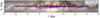 |
Fig. 4 Location of newly identified cluster candidates after screening (blue) and the known star clusters (red) in the Milky Way. |
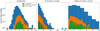 |
Fig. 5 Histograms of parameters for all candidates before screening (blue), for remaining candidates after screening (orange), and for known clusters (green). Top left: Overdensity. Top right: Number of member stars. Bottom left: Radius. |
2.5 Properties of individual clusters of interest
Some examples of extreme cluster candidates are shown in Fig. 6. The first is the largest (top row) and it is associated with dust emission in the longest wavelength bands. The second is the richest (middle row) and it is associated with a dark cloud. The third (bottom row) is the smallest in size and it stands out over the field stars as a compact group of bright sources. The three of them showcase the morphological features that we use to recognize a cluster candidate. One typical morphological feature is that the suspected members are inherently red, which is to be expected as we are searching for clusters in the inner Galaxy, subject to significant reddening along the line of sight, or extremely young objects that are still embedded in their parent dust clouds.
To demonstrate our candidates’ range of properties, we discuss three of the most extreme ones. Their verification plots, including CMDs and maps, are shown in Fig. 7 (from top to bottom).
GIPM 257 (l,b: 300.7463°, +0.0919°) is the largest cluster candidate from our search with a preliminary radius of 8.62′. There is an excess of redder sources within the cluster region, suggesting this is a site of ongoing star formation. Indeed, data from the Millimetre Astronomy Legacy Team 90 GHz Survey (MALT90; Foster et al. 2011; Jackson et al. 2013) helped to recognize this as a high-mass star-forming region with dense cores ([HJF2013] G300.747+00.096; Hoq et al. 2013) and young stellar objects (YSOs) (AGAL G300.748+00.097; Rathborne et al. 2016).
GIPM 402 (l,b: 335.436468°, −0.233556°) is the richest cluster candidate on our list. It contains the highest number of suspected members: 119 detected by the clustering algorithm and 209 within the search radius of the estimated radius of the cluster (2.76’). Previous observations have identified many YSOs (SSTGLMC G335.4318–00.2353 and others; Robitaille et al. 2008), dense cores (AGAL G335.441–00.237 and others; Contreras et al. 2013), and sub-millimeter sources ([LCW2019] GS335.4410–00.2323 and others; Lin et al. 2019), consistent with a young cluster. The three-color near- and mid-IR images suggest the presence of a dark cloud.
GIPM 8 (l,b: 0.5409°, +0.0262°) is the densest candidate identified by our search, where the density is the number of stars divided by cluster area. This is largely because this object appears compact on the sky with a radius of only 0.4′. We note that this surface density is different from the overdensity in units of the background root mean square (Eq. (1)), which is 2.8 for this object. The region is abundant with sub-millimeter (JCMTSE J174647.7–282708 and others; Di Francesco et al. 2008; Parsons et al. 2018) and X-ray sources (CXOGCS J174646.5–282708 and others; Muno et al. 2006). The sub-millimeter and X-ray emission may be emitted in dense cloud cores or originate from coronal activity in young stars (Parsons et al. 2018; Feigelson et al. 2007). Similarly to the previous candidates, the three-color near- and mid-IR images reveal the presence of dust around the cluster.
3 Cluster detection completeness
3.1 Generation of artificial clusters
We adopted an empirical approach to generate artificial clusters, instead of the traditional theoretical method that starts with a stellar initial mass function and radial surface density profiles to produce a fully synthetic object. We took the existing cluster Westerlund 2 with its well-known parameters as representative of its class, cleaned it statistically of contaminating field stars, and “moved” it to a larger distance, accounting for the increased crowding and increasing the extinction as appropriate. This method can only simulate clusters that are located further away than the prototype object, but it is model-independent and free from model-related biases.
First, we removed the field contamination from the sources in the region of the prototype cluster Westerlund 2. We adopted a cluster with a radius of 1′, then we defined an annulus (with the same area as the cluster region and centered on the cluster) where we sampled the field population for statistical decontamination of the cluster. Experiments show that the exact inner radius of the annulus is not critical, as long as we keep it within 1–2′ of the cluster region – the remaining number of stars after the decontamination changes at the level of a few percent. We chose to place the annulus next to the cluster region to minimize the effect of any large-scale stellar surface density variations across the field.
The actual decontamination was carried out in the CMD space – for each object in the field annulus, we removed the closest star in color and magnitude to the objects within the cluster region, starting from a random source, until one cluster object was removed for every object in the field annulus. The procedure is illustrated in Fig. 8, where for verification purposes we also show a decontamination of a pure field region where nearly all sources in the “cluster” region have been removed, as is expected.
The next step was to shift the “pure” Westerlund 2 population to a grid of predefined positions, extinctions, and reddenings where the artificial clusters would be located. This procedure is shown in Fig. 9. First, we corrected for the distance modulus and the extinction of Westerlund 2 itself – this is the move from the green to the blue points on the CMD (left panel). Then, the data must undergo three modifications: adding to the apparent magnitudes the respective distance modulus, adding to the color the reddening according to the extinction law of Rieke & Lebofsky (1985) – this is the move from the blue points to the red ones on the CMD – and accounting for the decreased angular separation between sources, because of the increased distance. The latter effect would have merged some nearby sources if they were observed with Spitzer at the newly adopted distance. These are marked with black dots on both panels and labeled as removed sources, although their flux was preserved and merged with nearby sources that are brighter than each of them. The flux merging uses Pogson’s law.
The condition to merge sources was based on a study of the GLIMPSE point source catalog in the inner Milky Way, to determine how close the nearest source can be as a function of the “primary” star’s magnitude: for [3.6]~8 mag the closest “secondaries” are usually at least ~4 arcsec away; for [3.6]~10 mag they are at least ~3 arcsec away; and for fainter stars they are at least ~2 arcsec away. Most likely these are projected binaries, not physical ones. We fit a linear relation through these three points and merger sources that come closer than this limit when we moved the prototype Westerlund 2 sources to the position of the newly injected artificial cluster. This a simplification, because we ignored the magnitudes of the primary and the secondary, but the experiments indicate that only a negligibly small fraction of sources are merged and that they have little effect on the cluster identification. This is related to the choice of the prototype cluster Westerlund 2. It is already fairly distant at ~4 kpc; the impact of the changing viewing geometry would have been much more significant if our prototype were closer, for example less than a kiloparsec from us, so the movement to the distance of the Galactic center would reduce the separations between stars by nearly an order of magnitude.
The grid was defined to place the artificial clusters in the innermost Galaxy – the region that is most difficult for cluster searches because of both crowding and extinction. We inserted clusters in 600 steps within the range −30≤l≤30 deg and in 12 steps within −0.5≤b≤0.5 deg, resulting in 7200 grid points. For each point, we carried out nine separate simulations, introducing artificial clusters subjected to all possible combinations of distances, D=6, 7, and 8 kpc, and visual extinctions, AV=11, 12, and 13 mag. In other words, this is a 3×3 grid. The choice of exact values is tentative, but they were selected to cover the ranges typical of the other massive clusters in this region. We limited the distances to span only the near side of the Milky Way. Higher extinctions have been found for clusters in young, dust-rich star-forming regions (e.g., Borissova et al. 2005, 2006) but not for supermassive clusters.
The artificial clusters were added on top of the stellar fields at the predefined locations. Unlike in the previous step, in which we merged starts that come too close together as the Westerlund 2 sources are moved further out to the adopted new distance, here we ignored the merging of the member stars and any field sources that may come too close to them, because a check indicated that ~2–4% of the suspected members are affected, even in the densest regions – typically less than one star per cluster.
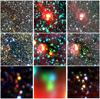 |
Fig. 6 Three color 2MASS JHKS, WISE W1W2W4, and GLIMPSE [3.6][4.5][8.0] (left to right) images for the most extreme objects in our sample: GIPM 257, the largest in size (top row; image size 16.6×16.6°), GIPM 402, the richest in terms of the number of suspected members (middle row; 5.5×5.5°), and the GIPM 8, the smallest in size (bottom row; 45×45″). North is always up, and east is to the left. |
3.2 Recovery of the artificial clusters
The same algorithm that was used for the cluster search was applied to the catalogs with the artificial clusters and the behavior of the recovery rates is shown in Fig. 10. The fraction of recovered clusters varies between 70 and 95%. Nearby clusters are easier to identify than more distant ones. However, the higher extinction seems to help in finding clusters – possibly because it sets the cluster in color space further apart from the contaminating foreground population that shows bluer colors than the candidate cluster member stars. The foreground dominates the surface density, but it is removed by the color criterion. An increase in AV by 1 mag roughly raises the recovery fraction by ~4%. Spatially, the innermost region at −2≤l≤2 deg stands out with a somewhat lower recovery rate, probably because of the worse crowding near the Galactic center. In Galactic latitude, there seems to be no drop in the recovery rate at the position of the Milky Way plane within the range of latitude, b, that is covered by our simulation.
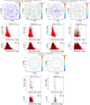 |
Fig. 7 Verification plots, similar to Fig. 2, for some of the most extreme candidates. See Sect. 2.5 for discussion of individual objects. |
4 Discussion and conclusions
We applied a new cluster finding algorithm – OPTICS – on the GLIMPSE survey point source catalog to identify obscured star clusters located in the inner Milky Way and report nearly 500 new objects; we also recovered about 140 previously identified ones. Importantly, these are all candidates, because without spectroscopy, proper motions, or parallaxes, it is impossible to verify their nature as bound systems. The deep spectroscopic surveys like the Multi-Object Optical and Near-infrared Spectrograph (MOONS; Cirasuolo et al. 2020), 4 metre Multi-Object Spectroscopic Telescope (4MOST; de Jong et al. 2019), and the Wide-field Spectroscopic Telescope (WST; Mainieri et al. 2024), and the near-IR astrometric space missions of the coming decades, will help to address this question. In particular, the future Roman Space Telescope will have wide-field near-IR imaging capabilities (e.g., Stauffer et al. 2018) that are ideal for carrying out a very deep survey of the Galactic plane at high resolution (see Paladini et al. 2023). Such a survey would not only discover thousands of new star clusters, enabling researchers to complete the census of them, but also confirm their true nature using proper motions.
The new OPTICS algorithm can handle the hierarchical structure of star formation but it has proved here to be not too important, because the severe field contamination in the direction of the inner Galaxy typically allows us to identify only the most compact obscured clusters; very few structures larger than 4–5 arcmin were identified. We speculate that the capability of the OPTICS algorithm to handle hierarchical structures will be important for studies of nearby galaxies like the Magellanic Clouds, M31, and M33. The classification and characterization of the new candidates remains outside the scope of this work but the properties of recovered known clusters do hint at the possibility that most of the new candidates would also be embedded and maybe a few would be highly obscured open or globular clusters. The distance estimates of these embedded clusters are not possible without proper spectroscopic or near-IR astrometric missions, and without this knowledge we cannot claim that our cluster candidates are bona fide clusters or not. So, while this new list is a step toward a more complete observational census of stellar clusters, this goal remains unattainable as our simulation shows, because the recovery rate for less massive, less rich, and less luminous clusters is bound to be lower than our estimates for clusters similar to Westerlund 2.
One challenge that remains to be addressed in future work is improving the field contamination removal. The member stars of the cluster or cluster candidates are more crowded than in the surrounding field. Therefore, the luminosity function in the cluster is shallower than in the field because of the source confusion. This may be one of the reasons – in addition to the stochastic or dark-cloud-related surface density variations – why do we sometimes have more stars in the sky annulus than in the cluster locus, as was mentioned in Sect. 2.4. An inspection of the clusters and field luminosity functions indicates that the small number of stars makes it difficult to determine the completeness limit and we have refrained from applying a completeness correction or even just removing the faint stars below some limit. This problem is similar to the edge detection issue in the tip of the red giant branch method of measuring extragalactic distances (Sakai et al. 1996). This method requires a large number of stars, which prevents its application to globular clusters. We have also refrained from applying an uncertain correction because the over-subtraction of the field stars reduces the recovery rate of our simulation, making our result more conservative.
Here, we have addressed the important but often neglected question of how successful our algorithm is in finding clusters with a simulation, adding semi-artificial clusters to the GLIMPSE point source catalog, and running the same search algorithm trying to recover them. As a first step, the simulation is limited to the most massive star clusters, with masses around 104 M⊙. It is semi-artificial because it is based on a real cluster – Westerlund 2 – which makes it model-independent. The simulation is also limited to the central part of our Galaxy, where the extinction is high and crowding is severe. The achieved recovery fraction is high – in the range of 70–95%, suggesting that the near side of the Milky Way may harbor ~1–3 additional supermassive star clusters. In other words, no large population of hidden supermassive clusters resides inside the Milky Way. The analysis of the simulated clusters indicates that the closer ones are easier to identify than their more distant counterparts, but the higher extinction often helps one to identify clusters, because it increases the color contrast between them and the contamination field population.
Our simulation is the first detailed one, after the initial attempts by Mercer et al. (2005), Ivanov et al. (2010) and Hanson et al. (2010). It needs to be extended to include lowermass and older clusters that have a larger impact on the stellar population in our Galaxy because of their higher numbers than the Westerlund 2-like clusters. An expansion toward near-IR sky surveys that typically have better angular resolution than the mid-IR surveys is another promising expansion avenue; for example, the VVV/X (Saito et al. 2024; Minniti et al. 2010). Last but not least, we underline again that the objects that the OPTICS algorithm identified are candidates and that further observations are needed to confirm their cluster nature.
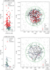 |
Fig. 8 Example of statistical decontamination of the cluster Westerlund 2 region (top) and an empty field nearby (bottom), shown to verify the removal procedure. The galactic coordinates of the two regions are marked at the top. The left panels show the GLIMPSE CMDs and the right ones the maps. The blue circles are all sources within the cluster radius (adopted 1′), the green circles all sources in an adjustment circular annulus (marked with green lines) with the same area as the cluster region, and the gray dots all sources outside both these two regions. The dotted black lines connect each removed cluster star with the corresponding field star. Solid red dots mark the remaining clusters of stars. The numbers in the legend give the number of each type of object. |
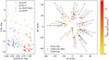 |
Fig. 9 Example of constructing an artificial cluster out of the “pure” Westerlund 2 population. The CMD is shown in the left panel. The green points mark the apparent position of the member stars as they are in Westerlund 2, the blue points indicate correction for reddening, and the red points reflect the additional reddening to the newly inserted artificial cluster. The distance modulus change was not applied here. The right panel shows the change in the apparent position of the member stars as they are “moved” from the distance of Westerlund 2 further out to the distance of the new artificial cluster. Black points on both panels are stars that were removed or merged because they came closer than the adopted limit to other stars that are brighter than them. For details, see Sect. 3.1. |
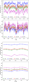 |
Fig. 10 Rate of artificial cluster recovery as a function of galactic coordinates for the entire sample, and for different distances, D, and visual extinctions, AV (labeled). For every value of D or AV, we averaged over the nine-element grid (see Sect. 3.1) along that value. |
Data availability
Full Table 3 is available at the CDS via anonymous ftp to cdsarc.cds.unistra.fr (130.79.128.5) or via https://cdsarc.cds.unistra.fr/viz-bin/cat/J/A+A/692/A194
Acknowledgements
This research has made use of the SIMBAD database, operated at CDS, Strasbourg, France. This research has made use of the VizieR catalog access tool, CDS, Strasbourg, France (Ochsenbein 1996). The original description of the VizieR service was published in Ochsenbein et al. (2000). This research has made use of the NASA/IPAC Infrared Science Archive, which is funded by the National Aeronautics and Space Administration and operated by the California Institute of Technology. The authors are grateful to LMU and ESO for the usage of computational facilities. The research of T.P. was supported by the Excellence Cluster ORIGINS, which is funded by the Deutsche Forschungsgemeinschaft (DFG, German Research Foundation) under Germany’s Excellence Strategy-EXC-2094-390783311. D.M. gratefully acknowledges support from the Center for Astrophysics and Associated Technologies CATA by the ANID BASAL projects ACE210002 and FB210003, and by Fondecyt Regular No. 1220724. We thank the anonymous referee for the helpful comments that helped to improve the manuscript greatly.
References
- Ankerst, M., Breunig, M. M., Kriegel, H.-P., & Sander, J. 1999, SIGMOD Rec., 28, 49 [CrossRef] [Google Scholar]
- Asa’d, R., Ivanov, V. D., Negueruela, I., et al. 2023, AJ, 165, 212 [CrossRef] [Google Scholar]
- Astropy Collaboration (Price-Whelan, A. M., et al.) 2018, AJ, 156, 123 [Google Scholar]
- Astropy Collaboration (Price-Whelan, A. M., et al.) 2022, ApJ, 935, 167 [NASA ADS] [CrossRef] [Google Scholar]
- Barbá, R. H., Roman-Lopes, A., Nilo Castellón, J. L., et al. 2015, A&A, 581, A120 [NASA ADS] [CrossRef] [EDP Sciences] [Google Scholar]
- Becklin, E. E., & Neugebauer, G. 1968, ApJ, 151, 145 [Google Scholar]
- Benjamin, R. A., Churchwell, E., Babler, B. L., et al. 2003, PASP, 115, 953 [Google Scholar]
- Bica, E., Dutra, C. M., Soares, J., & Barbuy, B. 2003, A&A, 404, 223 [NASA ADS] [CrossRef] [EDP Sciences] [Google Scholar]
- Borissova, J., Ivanov, V. D., Minniti, D., Geisler, D., & Stephens, A. W. 2005, A&A, 435, 95 [NASA ADS] [CrossRef] [EDP Sciences] [Google Scholar]
- Borissova, J., Ivanov, V. D., Minniti, D., & Geisler, D. 2006, A&A, 455, 923 [NASA ADS] [CrossRef] [EDP Sciences] [Google Scholar]
- Borissova, J., Bonatto, C., Kurtev, R., et al. 2011, A&A, 532, A131 [NASA ADS] [CrossRef] [EDP Sciences] [Google Scholar]
- Borissova, J., Ivanov, V. D., Lucas, P. W., et al. 2018, MNRAS, 481, 3902 [NASA ADS] [CrossRef] [Google Scholar]
- Camargo, D., Bica, E., & Bonatto, C. 2016, MNRAS, 455, 3126 [Google Scholar]
- Cirasuolo, M., Fairley, A., Rees, P., et al. 2020, The Messenger, 180, 10 [NASA ADS] [Google Scholar]
- Contreras, Y., Schuller, F., Urquhart, J. S., et al. 2013, A&A, 549, A45 [NASA ADS] [CrossRef] [EDP Sciences] [Google Scholar]
- Davies, B., Figer, D. F., Kudritzki, R.-P., et al. 2007, ApJ, 671, 781 [NASA ADS] [CrossRef] [Google Scholar]
- de Jong, R. S., Agertz, O., Berbel, A. A., et al. 2019, The Messenger, 175, 3 [NASA ADS] [Google Scholar]
- Di Francesco, J., Johnstone, D., Kirk, H., MacKenzie, T., & Ledwosinska, E. 2008, ApJS, 175, 277 [Google Scholar]
- Dutra, C. M., & Bica, E. 2001, A&A, 376, 434 [NASA ADS] [CrossRef] [EDP Sciences] [Google Scholar]
- Ester, M., Kriegel, H.-P., Sander, J., & Xu, X. 1996, in Proceedings of the Second International Conference on Knowledge Discovery and Data Mining, KDD’96 (AAAI Press), 226 [Google Scholar]
- Evans, I. N., Primini, F. A., Glotfelty, K. J., et al. 2010, ApJS, 189, 37 [NASA ADS] [CrossRef] [Google Scholar]
- Feigelson, E., Townsley, L., Güdel, M., & Stassun, K. 2007, in Protostars and Planets V, eds. B. Reipurth, D. Jewitt, & K. Keil (Tucson: University of Arizona Press), 313 [Google Scholar]
- Foster, J. B., Jackson, J. M., Barnes, P. J., et al. 2011, ApJS, 197, 25 [CrossRef] [Google Scholar]
- Hanson, M. M., Popescu, B., Larsen, S. S., & Ivanov, V. D. 2010, High. Astron., 15, 794 [NASA ADS] [Google Scholar]
- Hoq, S., Jackson, J. M., Foster, J. B., et al. 2013, ApJ, 777, 157 [Google Scholar]
- Hunter, J. D. 2007, Comput. Sci. Eng., 9, 90 [NASA ADS] [CrossRef] [Google Scholar]
- Hurt, R. L., Jarrett, T. H., Kirkpatrick, J. D., et al. 2000, AJ, 120, 1876 [Google Scholar]
- Ivanov, V. D., Borissova, J., Pessev, P., Ivanov, G. R., & Kurtev, R. 2002, A&A, 394, L1 [NASA ADS] [CrossRef] [EDP Sciences] [Google Scholar]
- Ivanov, V. D., Kurtev, R., & Borissova, J. 2005, A&A, 442, 195 [NASA ADS] [CrossRef] [EDP Sciences] [Google Scholar]
- Ivanov, V. D., Messineo, M., Zhu, Q., et al. 2010, IAU Symp., 266, 203 [NASA ADS] [Google Scholar]
- Jackson, J. M., Rathborne, J. M., Foster, J. B., et al. 2013, PASA, 30, e057 [Google Scholar]
- Kaltcheva, N. T., & Georgiev, L. N. 1993, MNRAS, 261, 847 [NASA ADS] [CrossRef] [Google Scholar]
- Koposov, S. E., Belokurov, V., & Torrealba, G. 2017, MNRAS, 470, 2702 [NASA ADS] [CrossRef] [Google Scholar]
- Kurtev, R., Ivanov, V. D., Borissova, J., & Ortolani, S. 2008, A&A, 489, 583 [NASA ADS] [CrossRef] [EDP Sciences] [Google Scholar]
- Lada, C. J., & Lada, E. A. 2003, ARA&A, 41, 57 [Google Scholar]
- Lin, Y., Csengeri, T., Wyrowski, F., et al. 2019, A&A, 631, A72 [NASA ADS] [CrossRef] [EDP Sciences] [Google Scholar]
- Mainieri, V., Anderson, R. I., Brinchmann, J., et al. 2024, arXiv e-prints [arXiv:2403.05398] [Google Scholar]
- Mercer, E. P., Clemens, D. P., Meade, M. R., et al. 2005, ApJ, 635, 560 [NASA ADS] [CrossRef] [Google Scholar]
- Minniti, D., Lucas, P. W., Emerson, J. P., et al. 2010, New A, 15, 433 [Google Scholar]
- Minniti, D., Hempel, M., Toledo, I., et al. 2011, A&A, 527, A81 [NASA ADS] [CrossRef] [EDP Sciences] [Google Scholar]
- Minniti, D., Fernández-Trincado, J. G., Smith, L. C., et al. 2021a, A&A, 648, A86 [NASA ADS] [CrossRef] [EDP Sciences] [Google Scholar]
- Minniti, D., Palma, T., Camargo, D., et al. 2021b, A&A, 652, A129 [NASA ADS] [CrossRef] [EDP Sciences] [Google Scholar]
- Moffat, A. F. J., Shara, M. M., & Potter, M. 1991, AJ, 102, 642 [NASA ADS] [CrossRef] [Google Scholar]
- Morales, E. F. E., Wyrowski, F., Schuller, F., & Menten, K. M. 2013, A&A, 560, A76 [NASA ADS] [CrossRef] [EDP Sciences] [Google Scholar]
- Muno, M. P., Bauer, F. E., Bandyopadhyay, R. M., & Wang, Q. D. 2006, ApJS, 165, 173 [NASA ADS] [CrossRef] [Google Scholar]
- Nagata, T., Woodward, C. E., Shure, M., Pipher, J. L., & Okuda, H. 1990, ApJ, 351, 83 [NASA ADS] [CrossRef] [Google Scholar]
- Nagata, T., Hyland, A. R., Straw, S. M., Sato, S., & Kawara, K. 1993, ApJ, 406, 501 [NASA ADS] [CrossRef] [Google Scholar]
- Nagata, T., Woodward, C. E., Shure, M., & Kobayashi, N. 1995, AJ, 109, 1676 [NASA ADS] [CrossRef] [Google Scholar]
- Nambiar, S., Das, S., Vig, S., & Gorthi, R. S. S. 2019, MNRAS, 482, 3789 [NASA ADS] [CrossRef] [Google Scholar]
- Ochsenbein, F. 1996, The VizieR database of astronomical catalogues [Google Scholar]
- Ochsenbein, F., Bauer, P., & Marcout, J. 2000, A&AS, 143, 23 [NASA ADS] [CrossRef] [EDP Sciences] [Google Scholar]
- Okuda, H., Shibai, H., Nakagawa, T., et al. 1990, ApJ, 351, 89 [NASA ADS] [CrossRef] [Google Scholar]
- Paladini, R., Zucker, C., Benjamin, R., et al. 2023, arXiv e-prints [arXiv:2307.07642] [Google Scholar]
- Parsons, H., Dempsey, J. T., Thomas, H. S., et al. 2018, ApJS, 234, 22 [Google Scholar]
- Parzen, E. 1962, Ann. Math. Stat., 33, 1065 [Google Scholar]
- Platais, I., Kozhurina-Platais, V., & van Leeuwen, F. 1998, AJ, 116, 2423 [NASA ADS] [CrossRef] [Google Scholar]
- Portegies Zwart, S. F., McMillan, S. L. W., & Gieles, M. 2010, ARA&A, 48, 431 [NASA ADS] [CrossRef] [Google Scholar]
- Preibisch, T., Kim, Y.-C., Favata, F., et al. 2005, ApJS, 160, 401 [NASA ADS] [CrossRef] [Google Scholar]
- Rathborne, J. M., Whitaker, J. S., Jackson, J. M., et al. 2016, PASA, 33, 030 [NASA ADS] [CrossRef] [Google Scholar]
- Rieke, G. H., & Lebofsky, M. J. 1985, ApJ, 288, 618 [Google Scholar]
- Robitaille, T. P., Meade, M. R., Babler, B. L., et al. 2008, AJ, 136, 2413 [NASA ADS] [CrossRef] [Google Scholar]
- Ryu, J., & Lee, M. G. 2018, ApJ, 856, 152 [NASA ADS] [CrossRef] [Google Scholar]
- Saito, R. K., Hempel, M., Alonso-García, J., et al. 2024, A&A, 689, A148 [NASA ADS] [CrossRef] [EDP Sciences] [Google Scholar]
- Sakai, S., Madore, B. F., & Freedman, W. L. 1996, ApJ, 461, 713 [Google Scholar]
- Skrutskie, M. F., Cutri, R. M., Stiening, R., et al. 2006, AJ, 131, 1163 [NASA ADS] [CrossRef] [Google Scholar]
- Solin, O., Ukkonen, E., & Haikala, L. 2012, A&A, 542, A3 [Google Scholar]
- Spitzer Science, C. 2009, VizieR Online Data Catalog: II/293 [Google Scholar]
- Stauffer, J., Helou, G., Benjamin, R. A., et al. 2018, arXiv e-prints [arXiv:1806.00554] [Google Scholar]
- Trumpler, R. J. 1930, Lick Observ. Bull., 420, 154 [CrossRef] [Google Scholar]
- Westerlund, B. 1961a, PASP, 73, 51 [NASA ADS] [CrossRef] [Google Scholar]
- Westerlund, B. 1961b, Arkiv for Astronomi, 2, 419 [Google Scholar]
- Wright, E. L., Eisenhardt, P. R. M., Mainzer, A. K., et al. 2010, AJ, 140, 1868 [Google Scholar]
- Zeidler, P., Sabbi, E., Nota, A., et al. 2015, AJ, 150, 78 [NASA ADS] [CrossRef] [Google Scholar]
- Zeidler, P., Sabbi, E., Nota, A., & McLeod, A. F. 2021, AJ, 161, 140 [NASA ADS] [CrossRef] [Google Scholar]
All Tables
Some of the screened cluster candidates. The entire table is available at the CDS.
All Figures
|
Fig. 1 Distribution of candidate cluster sizes for different search parameters. |
| In the text | |
|
Fig. 2 Cluster candidate verification plots for a known recovered cluster (G3CC 8; Morales et al. 2013, left) and for a new candidate (right). The titles list the derived cluster parameters (see Sects. 2.3 and 3 for more details). Panels: Top left – Mid-IR CMD; red dots are all sources within the cluster radius and black dots are all sources in the sky annulus. Top right – Map of GLIMPSE sources with colors in the bin 0.6 mag≤[3.6]−[4.5]≤4.0 mag, color-coded by [3.6]−[4.5]. The red circle shows the cluster region and the black rings the sky annulus. Middle left – Combined near/mid-IR CMD; the dots are coded lines in the panel above. Middle right – Map of GLIMPSE-2MASS sources. Black dots represent all sources, while larger dots color-coded by [K]−[3.6] are the objects with 0.6 mag≤[3.6]−[4.5]≤4.0 mag. Bottom left – Mid-IR [3.6]−[4.5] color histogram for sources in the cluster region (black) and sources in the background annulus (red). The potential cluster members cause the excess at 0.6 mag≤[3.6]−[4.5]≤4.0 mag. Bottom right – Near/mid-IR K-[3.6] color histogram. The notation is the same as on the previous histogram. Vertical dashed blue lines at K−[4.5]=1.0 mag and 4.0 mag were added only to guide the eye. The potential cluster members cause the excess at K−[4.5]≥1.0 mag. |
| In the text | |
|
Fig. 3 Three color images (2.5′ on the side) for the cluster in Fig. 2 (left): 2MASS JHKS, WISE W1W2W4 and GLIMPSE [3.6][4.5][8.0] (left to right). North is up, east is to the left. |
| In the text | |
|
Fig. 4 Location of newly identified cluster candidates after screening (blue) and the known star clusters (red) in the Milky Way. |
| In the text | |
|
Fig. 5 Histograms of parameters for all candidates before screening (blue), for remaining candidates after screening (orange), and for known clusters (green). Top left: Overdensity. Top right: Number of member stars. Bottom left: Radius. |
| In the text | |
|
Fig. 6 Three color 2MASS JHKS, WISE W1W2W4, and GLIMPSE [3.6][4.5][8.0] (left to right) images for the most extreme objects in our sample: GIPM 257, the largest in size (top row; image size 16.6×16.6°), GIPM 402, the richest in terms of the number of suspected members (middle row; 5.5×5.5°), and the GIPM 8, the smallest in size (bottom row; 45×45″). North is always up, and east is to the left. |
| In the text | |
|
Fig. 7 Verification plots, similar to Fig. 2, for some of the most extreme candidates. See Sect. 2.5 for discussion of individual objects. |
| In the text | |
|
Fig. 8 Example of statistical decontamination of the cluster Westerlund 2 region (top) and an empty field nearby (bottom), shown to verify the removal procedure. The galactic coordinates of the two regions are marked at the top. The left panels show the GLIMPSE CMDs and the right ones the maps. The blue circles are all sources within the cluster radius (adopted 1′), the green circles all sources in an adjustment circular annulus (marked with green lines) with the same area as the cluster region, and the gray dots all sources outside both these two regions. The dotted black lines connect each removed cluster star with the corresponding field star. Solid red dots mark the remaining clusters of stars. The numbers in the legend give the number of each type of object. |
| In the text | |
|
Fig. 9 Example of constructing an artificial cluster out of the “pure” Westerlund 2 population. The CMD is shown in the left panel. The green points mark the apparent position of the member stars as they are in Westerlund 2, the blue points indicate correction for reddening, and the red points reflect the additional reddening to the newly inserted artificial cluster. The distance modulus change was not applied here. The right panel shows the change in the apparent position of the member stars as they are “moved” from the distance of Westerlund 2 further out to the distance of the new artificial cluster. Black points on both panels are stars that were removed or merged because they came closer than the adopted limit to other stars that are brighter than them. For details, see Sect. 3.1. |
| In the text | |
|
Fig. 10 Rate of artificial cluster recovery as a function of galactic coordinates for the entire sample, and for different distances, D, and visual extinctions, AV (labeled). For every value of D or AV, we averaged over the nine-element grid (see Sect. 3.1) along that value. |
| In the text | |
Current usage metrics show cumulative count of Article Views (full-text article views including HTML views, PDF and ePub downloads, according to the available data) and Abstracts Views on Vision4Press platform.
Data correspond to usage on the plateform after 2015. The current usage metrics is available 48-96 hours after online publication and is updated daily on week days.
Initial download of the metrics may take a while.