| Issue |
A&A
Volume 597, January 2017
|
|
|---|---|---|
| Article Number | A9 | |
| Number of page(s) | 16 | |
| Section | Stellar structure and evolution | |
| DOI | https://doi.org/10.1051/0004-6361/201629349 | |
| Published online | 19 December 2016 | |
VLTI/AMBER spectro-interferometry of the late-type supergiants V766 Cen (=HR 5171 A), σ Oph, BM Sco, and HD 206859 ⋆
1 ESO, Karl-Schwarzschild-Str. 2, 85748 Garching bei München, Germany
e-mail: This email address is being protected from spambots. You need JavaScript enabled to view it.
2 Dpt. Astronomia i Astrofísica, Universitat de València, C/Dr. Moliner 50, 46100 Burjassot, Spain
3 Instituto de Astrofísica de Andalucía (IAA-CSIC), Glorieta de la Astronomía S/N, 18008 Granada, Spain
4 Centro Astronómico Hispano Alemán, Calar Alto, (CSIC-MPG), Sierra de los Filabres, 04550 Gergal, Spain
5 Laboratoire Lagrange, UMR 7293, Université de Nice Sophia-Antipolis, CNRS, Observatoire de la Côte d’Azur, BP. 4229, 06304 Nice Cedex 4, France
6 Observatorio Astronómico, Universidad de València, 46980 Paterna, València, Spain
Received: 20 July 2016
Accepted: 3 October 2016
Abstract
Aims. We add four warmer late-type supergiants to our previous spectro-interferometric studies of red giants and supergiants.
Methods. We measure the near-continuum angular diameter, derive fundamental parameters, discuss the evolutionary stage, and study extended atmospheric atomic and molecular layers.
Results. V766 Cen (=HR 5171 A) is found to be a high-luminosity (log L/L⊙ = 5.8 ± 0.4) source of effective temperature 4290 ± 760 K and radius 1490 ± 540 R⊙, located in the Hertzsprung-Russell (HR) diagram close to both the Hayashi limit and Eddington limit; this source is consistent with a 40 M⊙ evolutionary track without rotation and current mass 27–36 M⊙. V766 Cen exhibits Na i in emission arising from a shell of radius 1.5 RPhot and a photocenter displacement of about 0.1 RPhot. It shows strong extended molecular (CO) layers and a dusty circumstellar background component. The other three sources are found to have lower luminosities of about log L/L⊙ = 3.4–3.5, corresponding to 5–9 M⊙ evolutionary tracks. They cover effective temperatures of 3900 K to 5300 K and radii of 60–120 R⊙. They do not show extended molecular layers as observed for higher luminosity RSGs of our sample. BM Sco shows an unusually strong contribution by an over-resolved circumstellar dust component.
Conclusions. V766 Cen is a red supergiant located close to the Hayashi limit instead of a yellow hypergiant already evolving back toward warmer effective temperatures as discussed in the literature. Our observations of the Na i line and the extended molecular layers suggest an optically thick pseudo-photosphere at about 1.5 RPhot at the onset of the wind. The stars σ Oph, BM Sco, and HD 206859 are more likely high-mass red giants instead of RSGs as implied by their luminosity class Ib. This leaves us with an unsampled locus in the HR diagram corresponding to luminosities log L/L⊙ ~ 3.8–4.8 or masses 10–13 M⊙, possibly corresponding to the mass region where stars explode as (type II-P) supernovae during the red supergiant stage. With V766 Cen, we now confirm that our previously found relation of increasing strength of extended molecular layers with increasing luminosities extends to double our previous luminosities and up to the Eddington limit. This might further point to steadily increasing radiative winds with increasing luminosity.
Key words: techniques: interferometric / supergiants / stars: atmospheres / stars: mass-loss / stars: individual: V766 Cen / stars: individual: BM Sco
Based on observations made with the VLT Interferometer (VLTI) at Paranal Observatory under program ID 093.D-0014.
© ESO, 2016
1. Introduction
Red supergiants (RSGs) are cool evolved massive stars before their transition toward Wolf-Rayet (WR) stars and core-collapse supernovae (SNe). Their characterization and location in the Hertzsprung-Russell (HR) diagram are of importance to calibrate stellar evolutionary models for massive stars and to understand their further evolution toward WR stars and SNe, a topic that has seen an increased interest (e.g., Dessart et al. 2013; Smith 2014; Meynet et al. 2015). In addition the structure and morphology of the close circumstellar environment and wind regions, including the atmospheric molecular layers and dusty envelopes, are currently a matter of debate (e.g., Josselin & Plez 2007; de Wit et al. 2008; Smith et al. 2009; Verhoelst et al. 2009; Yoon & Cantiello 2010; Walmswell & Eldridge 2012). Knowledge of the circumstellar envelope, along with the knowledge of the fundamental parameters, is important to understand the matching of SN progenitors to the different types of core-collapse SNe (e.g., Heger et al. 2003; Groh et al. 2013).
This paper is conceived as the fourth in a series of previous papers in which we have been studying the fundamental parameters and extended atmospheric layers of nearby late-type supergiants based on spectro-imaging with the VLTI/ AMBER instrument, including those by Wittkowski et al. (2012), Arroyo-Torres et al. (2013), and Arroyo-Torres et al. (2015), along with a similar study of lower mass red giants (Arroyo-Torres et al. 2014). Our sample thus far included the late-K- and M-type RSGs VY CMa (spectral type M3-4 II), AH Sco (M5 Ia-Iab), UY Sct (M4 Ia), KW Sgr (M4 Ia), V602 Car (M3 Ia-Iab), HD 95687 (M2 Ia), and HD 183589 (K5 III), along with five lower mass giants. We use spectral types as adopted by Simbad throughout this paper; in some cases different spectral classifications are available in the literature. We showed that extended molecular atmospheres with extensions comparable to Mira variable asymptotic giant branch (AGB) stars are a common feature of luminous RSGs, and that – unlike for Miras – this phenomenon is not predicted by current 3D convection or 1D pulsation models. We found a correlation of the contribution by extended atmospheric layers with luminosity, which may support a scenario of radiative acceleration on Doppler-shifted molecular lines as suggested by Josselin & Plez (2007). However, the processes that levitate the atmospheres of RSGs to observed extensions currently remain unknown.
In this paper, we add four warmer supergiants of spectral types G5 to K2.5 to our sample. These sources include the late-type supergiants V766 Cen (=HR 5171 A, Simbad spectral type G8 Ia), σ Oph (K2 III), BM Sco (K2 Ib), and HD 206859 (G5 Ib). V766 Cen (=HR 5171 A) was classified as a yellow hypergiant (YHG) by Humphreys et al. (1971), van Genderen (1992), and de Jager (1998), showing an intense optically thin silicate emission feature (Humphreys et al. 1971). The star is known to have a companion (HR 5171 B) at a separation of 9.7′′, which was classified as B0 Ib. Warren (1973) reported on the existence of a high temperature, low-density envelope based on the detection of weak nebular [N II] emission. Chesneau et al. (2014) suggested that V766 Cen (=HR 5171 A) itself has a low-mass companion that is very close to the primary star, possibly in the common-envelope phase. BM Sco (=HD 160371) is a K2.5 supergiant from the sample of Levesque et al. (2005), who aimed at characterizing the temperature scale of galactic RSGs using spectro-photometry. HD 206859 is a G5 supergiant from the sample of van Belle et al. (2009), who measured effective temperatures and linear radii of a sample of galactic RSGs with the Palomar Testbed Interferometer (PTI) in the H and K bands. The stars σ Oph, BM Sco, and HD 206859 are included in the sample of McDonald et al. (2012), who derived temperatures, luminosities, and infrared excesses of Hipparcos stars by comparing model atmospheres to SEDs. We aim to study the properties of these individual sources by direct spectro-interferometry. Altogether, they increase our sample significantly. In particular we aim to study whether or not the presence of extended molecular layers and the correlation of the contribution by extended atmospheric layers with luminosity reaches the level of warmer and more luminous late-type supergiants.
2. Observations and data reduction
We observed the late-type supergiants V766 Cen (=HR 5171 A), σ Oph, BM Sco, and HD 206859 with the ESO Very Large Telescope Interferometer (VLTI), utilizing three of the auxiliary telescopes of 1.8 m diameter, and the Astronomical Multi-BEam combineR (AMBER) instrument with the external fringe tracker FINITO (Petrov et al. 2007). We employed the medium-resolution mode (R ~ 1500) in the K-2.1 μm and K-2.3 μm bands. We observed the data as sequences of calbefore-sci-calafter. Our calibrators were HIP 72135 (RA 14 45 18.8, Dec –51 18 54, spectral type K4 III, angular diameter 1.76 mas), HIP 87846 (RA 17 56 47.4, Dec –44 20 32, K2 III, 1.92 mas), HIP 87491 (RA 17 52 35.4, Dec +01 18 18, K5 III, 2.46 mas), HIP 88101 (RA 17 59 36.8, Dec –04 49 16, K5 III, 2.24 mas), and HIP 109068 (RA 22 05 40.7, Dec +05 03 31, K4 III, 2.39 mas). The calibrators were selected from the ESO Calibration Selector CalVin, in turn based on the catalog by Lafrasse et al. (2010).
Table 1 shows the details of our observations including the calibrator used in each case. Some sources are listed with only one calibrator, in cases where the data quality of the second calibrator observation was low and we could not use it.
It is essential for a good calibration of the interferometric transfer function that the performance of the FINITO fringe tracking is comparable between the corresponding calibrator and science target observations. Optical path fluctuations (jitter) produce fringe motions during the recording of one AMBER frame. These motions reduce the squared visibility by a factor e−σφ2, where σφ is the fringe phase standard deviation over the frame recording time (more information in the AMBER User Manual1). This attenuation is corrected by the interferometric transfer function only if σφ was comparable between science and calibrator observations. We thus inspected the mean FINITO phase rms values to confirm that they were comparable. In some cases we deselected individual files for which this factor deviated by more than about 20%. In some cases we had to discard a complete data set because the FINITO phase rms values were systematically very different between the science target observation and calibrator observations.
We obtained raw visibility data from our selected AMBER observations using version 3.0.8 of the amdlib data reduction package (Tatulli et al. 2007; Chelli et al. 2009). We appended the visibility data of all scans of the same source taken consecutively, and we selected and averaged the resulting visibilities using appropriate criteria. We selected all frames that have flux densities that are three times higher than the noise and 80% of the remaining frames with best signal-to-noise ratio (S/N)2.
For the last reduction steps, we used scripts of IDL (Interactive Data Language), which we developed. First, we performed the absolute wavelength calibration by correlating the AMBER flux spectra with a reference spectrum, that of the star BS 4432 (spectral type K4.5 III, similar to our calibrators), from Lançon & Wood (2000). Afterward, we calibrated the flux and visibility spectra. The relative flux calibration was performed with the instrumental response, which is estimated by the calibrators and the BS 4432 spectrum. The visibility calibration was performed as in our previous work (Arroyo-Torres et al. 2013, 2014).
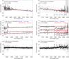 |
Fig. 1 Left (from top to bottom): observed (black) normalized flux, squared visibility amplitudes, and closure phases of V766 Cen obtained with the MR-K 2.1 μm setting on 2014 April 07. Right: same as left but obtained with the MR-K 2.3 μm setting on 2014 April 07. The black solid lines connect all the observed data points, while for the sake of clarity, the “X” symbols and associated error bars are shown for only every fifth data point. The blue curves show the best-fit UD model, and the red curves the best-fit PHOENIX model prediction. The visibility plots (middle panels) show three curves, one for each of the three baselines of the AMBER triangle. (cf. Sect. 3.2). |
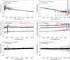 |
Fig. 2 As Fig. 1, but for data of σ Oph obtained with the MR-K 2.1 μm setting on 2014 April 25 (left) and with the MR-K 2.3 μm setting on 2014 April 07 (right). |
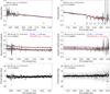 |
Fig. 3 As Fig. 1, but for data of BM Sco obtained with the MR-K 2.1 μm setting on 2014 April 25 (left) and with the MR-K 2.3 μm setting on 2014 April 07 (right). |
3. Results
Figures 1–5 show the resulting reduced data for each of the data sets listed in Table 1. The data include the normalized flux, the squared visibility amplitudes for each baseline, and the closure phases. All quantities are plotted versus wavelength. The figures also show the predictions by a uniform-disk (UD) model and by PHOENIX model atmospheres as discussed below in Sect. 3.2. All targets show relatively flat flux spectra, decreasing with wavelength, and with CO absorption features from 2.3 μm onward, which is typical for late-type supergiants. The spectral features at the edges of the K band below about 2.0 μm and above about 2.4 μm are most likely from noise owing to the lower instrumental and atmospheric transmission at these wavelengths. Among our four sources, the CO features in the flux spectra are relatively weak for V766 Cen and HD 206859, and stronger for σ Oph and BM Sco. This is consistent with the warmer spectral types of G8/G5 for V766 Cen/HD 206859, compared to K2 for σ Oph and BM Scou. However, the spectrum of V766 Cen may be a composite spectrum including the suggested close companion, cf. Sect. 3.1.1. However, in the visibility spectra, the CO features are very strong for V766 Cen, indicating that CO is formed at significantly higher layers in an extended atmosphere compared to the continuum. For the other targets, CO features are weak in the visibility spectra of BM Sco, and are absent for σ Oph and HD 206859, indicating that CO is formed only slightly above or at about the same layers as the continuum.
The closure phase of V766 Cen (bottom panels of Fig. 1) shows significant variations at the positions of the CO bandheads between 2.3 μm and 2.5 μm, indicating deviations from point symmetry at the CO-forming extended layers. Chesneau et al. (2014) showed similar results in their Figs. B.1 and B.2. The closure phase data of σ Oph, BM Sco, and HD 206859 do not show any significant deviations from point symmetry at any wavelength. However, since our measurements lie in the first lobe of the visibility, we cannot exclude asymmetries on scales smaller than the photospheric stellar disk.
Our flux spectra of V766 Cen exhibit an emission feature at a wavelength of 2.205 μm, which was also noticed by Chesneau et al. (2014) and identified as the Na i doublet. It corresponds to significant drops in the visibility, indicating that Na i is formed at higher atmospheric layers compared to the continuum. A more detailed study of this feature follows below in Sect. 3.3. This feature is not visible for any of the other sources. There are no other significant spectral features visible in the flux or visibility spectra of our sources within our S/N.
VLTI/AMBER observations.
3.1. Estimates of bolometric fluxes and distances
In order to derive fundamental parameters of our sources based on the measured angular diameters derived below, we need to estimate bolometric flux values and distances as a prerequisite.
3.1.1. Bolometric fluxes
We estimated the bolometric flux of each of our sources by integrating broadband photometry available in the literature. The details of our procedure are described in Arroyo-Torres et al. (2014, Sect. 4.2). We used B and V magnitudes from Kharchenko (2001), J, H, K magnitudes from Cutri et al. (2003), and the IRAS fluxes from Beichman et al. (1988) for V766 Cen, BM Sco, and HD 206859 and from Moshir et al. (1990) for σ Oph. We dereddened the flux value using an estimated EB−V value. For V766 Cen and HD 206859, we used the V−K color excess method with intrinsic colors from Ducati et al. (2001). For σ Oph and BM Sco, we used the values estimated by Schlafly & Finkbeiner (2011) and Levesque et al. (2005), respectively. The adopted EB−V values are 0.12 for σ Oph, 0.14 for BM Sco, 0.10 for HD 206859, and 0.92 for V766 Cen. We assume an uncertainty of 15% in the final bolometric flux.
For V766 Cen, we estimate a total bolometric flux of 2.25 × 10⁻⁹ W/m2. This value includes the contribution by the close companion that was suggested by Chesneau et al. (2014). Given the effective temperature of the companion of 4811 K and its angular diameter of 1.8 mas from Chesneau et al. (2014), we estimate a flux contribution of the companion of 5.78 × 10⁻¹⁰ W/m2 and conservatively adopt an error of 50%. Subtracting this value from the total flux, we derive a bolometric flux of the primary component alone of 1.68 × 10⁻⁹ W/m2±0.45 × 10-9 W/m2.
3.1.2. Distances
V766 Cen belongs to the OB association R80, and we adopted its distance by Humphreys (1978). For BM Sco, we used the distance of the OB association M6 (Mermilliod & Paunzen 2003). The stars σ Oph and HD 206859 are not known to belong to any OB association. We used the distance from Anderson & Francis (2012). The adopted distances are listed in Table 3.
3.2. Model atmosphere fits
We modeled our visibility data using a uniform disk (UD) model as well as PHOENIX model atmospheres following our previous papers (Wittkowski et al. 2012; Arroyo-Torres et al. 2013, 2015): we used the grid of PHOENIX model atmospheres that we introduced in Arroyo-Torres et al. (2013). We used a scaled visibility function of the form  (1)where A accounts for the flux fraction of the stellar disk, and where the remaining flux is attributed to a possible over-resolved circumstellar component within our field of view. The AMBER field of view using the ATs is about 270 mas in size. The Rosseland angular diameter ΘRoss of the respective PHOENIX model was the only fit parameter in addition to A. Here, ΘRoss corresponds to that model layer where the Rosseland optical depth equals 2/3. Likewise, we used a scaled UD model with fit parameters A and ΘUD. While we have shown that none of the currently available model atmospheres predict observed extensions of molecular layers (mainly in CO lines), our previous data (Wittkowski et al. 2012; Arroyo-Torres et al. 2013, 2015) as well as other studies (e.g., Perrin et al. 2004) showed that visibility curves of RSGs in near-continuum bandpasses can be well described by UD curves or hydrostatic model atmospheres. As a result, we restricted the model fits to the near-continuum band at 2.05 μm–2.20 μm, which is least affected by contamination from molecular layers within the K band. This bandpass also avoids the Na i doublet that has been detected for V766 Cen. We chose initial parameters of the PHOENIX model (mass M, effective temperature Teff, luminosity L) and iterated so that the model parameters were consistent with those derived from the Rosseland angular diameters and the adopted bolometric fluxes and distances. Finally, for V766 Cen, σ Oph, BM Sco, HD 206859, we used model atmospheres with effective temperatures 4300 K, 4100 K, 3900 K, 5300 K, and log g of values –0.5, 1, 1, 2, respectively. We used models of masses 1 M⊙ and 20 M⊙ for all sources because our model grid includes only these masses. The structure of the atmosphere is not very sensitive to mass (Hauschildt et al. 1999) and the differences in our final ΘRoss values are small compared to the quoted errors. The ΘRoss values are the only fit results that are used in the following. Table 2 shows the resulting best-fit angular diameters ΘRoss/ ΘUD and flux fractions A.
Figure 6 shows for each of our sources the near-continuum (averaged over 2.05 μm–2.20 μm) squared visibility amplitudes as a function of spatial frequency together with the best-fit PHOENIX and UD models. V766 Cen and BM Sco show A values significantly below 1, indicating the presence of an underlying over-resolved component within our field of view, possibly due to dust.
Best-fit flux fractions and angular diameters.
To realistically estimate the error of the angular diameter, including statistical and systematic errors, we applied variations of the angular diameter so that the model visibility curve lies below and on top of all measured points. These maximum and minimum visibility curves are plotted as dashed lines in Fig. 6. For V766 Cen (top panel of Fig. 6), we also used the medium spectral resolution K-band data obtained by Chesneau et al. (2014) on 2012-03-09 in addition to our own data. We processed them in the same way as our data. We did not use the low spectral resolution data from Chesneau et al. (2014) for consistency with our strategy of basing our study on the medium spectral resolution mode.
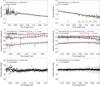 |
Fig. 5 As Fig. 1, but for data of HD 206859 obtained with the MR-K 2.1 μm setting on 2014 June 20 (left) and with the MR-K 2.3 μm setting on 2014 June 25 (right). |
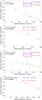 |
Fig. 6 Average of squared visibility amplitudes taken in the near-continuum bandpass at 2.05–2.20 μm for (from top to bottom) V766 Cen, σ Oph, BM Sco, and HD 206859 as a function of spatial frequency. The red lines indicate the best-fit UD models and the blue lines the best-fit PHOENIX models. The dashed lines are the maximum and minimum visibility curves, from which we estimated the errors of the angular diameters. |
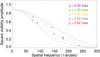 |
Fig. 7 Influence of the close companion of V766 Cen on the visibility curve. The asterisk and diamond symbols denote our near-continuum (2.05–2.20 μm) data, the central dashed line denotes the best-fit UD with over-resolved component, and the dash-dotted lines the error of the UD diameter. The color curves show the synthetic visibilities of a binary toy model consisting of two UDs and an over-resolved component with flux ratios as derived by Chesneau et al. (2014). The different colors indicate different positions of the companion corresponding along the projected orbit. The figure illustrates that our observations cannot separate between these curves and thus cannot fully characterize the companion. The range of the visibility curves of our binary toy model are within our already adopted diameter error. |
Moreover, for V766 Cen, we needed to investigate the effect that the suggested close companion (Chesneau et al. 2014) may have on our visibility data and on the determination of the angular diameter of the primary (cf. the corresponding discussion for the bolometric flux in Sect. 3.1.1.) We used a binary toy model, consisting of two UDs, one UD for the primary and one offset UD for the close companion, and an over-resolved component. We used the parameters of the orbit as obtained with the best NIGHTFALL model by Chesneau et al. (2014)3. Since we do not know the exact position along the orbit at the time of our observation, we computed synthetic visibility values for a range of such positions. Figure 7 shows the resulting synthetic visibility values compared to the measured values along with the uncertainties due to our UD analysis described above. As seen in the figure, the additional error introduced by the presence of the close companion is comparable to that of our UD analysis. Accordingly, we added in quadrature both contributions to the final uncertainty and, in practice, we multiplied our error from the UD analysis by a factor of  .
.
Finally, we used the best-fit PHOENIX models to produce synthetic flux and visibility data as a function of wavelength. These are shown in Figs. 1–5 together with the observed data.
For all four sources, the synthetic flux spectra (top panels) of the PHOENIX model are generally in good agreement with our observations, in particular at the locations of the CO bandheads. The PHOENIX model fluxes are consistent with the stronger CO bands for σ Oph and BM Sco, and the weaker CO bands for V766 Cen and HD 206859. For V766 Cen, the observed CO features may be weaker than predicted. It is not clear whether this is due to noise or the composite spectrum with the close companion, which the model does not take into account. The observed presence of the Na i doublet in emission for V766 Cen is not reproduced by the model atmosphere.
The visibility spectra (middle panels of Figs. 2–5) agree between observations and models for σ Oph, BM Sco, and HD 206859; both the observed and model visibility spectra do not show significant CO features, indicating that CO is formed close to the photosphere. BM Sco shows weak CO features that slightly extend those of the best-fit PHOENIX model. It is not yet clear whether this indicates an extension of the CO layers beyond the predictions of the model for this source or whether, for example, assumptions on the distance or bolometric flux and, thus of model parameters, are erroneous.
However, the visibility spectra of V766 Cen (middle panels of Fig. 1) show large visibility drops in the CO bandheads (2.3–2.5 μm) and in the Na i doublet (2.205 μm), which are not reproduced by the PHOENIX model. The synthetic PHOENIX visibilities show CO features, but these features are much weaker. This indicates that the PHOENIX model structure is too compact compared to our observations. We observed the same phenomenon previously for other RSGs as follows: VY CMa (Wittkowski et al. 2012), AH Sco, UY Sct, KW Sgr (Arroyo-Torres et al. 2013), and V602 Car, HD 95687 (Arroyo-Torres et al. 2015).
The panels showing the closure phases (bottom panels) do not include model atmosphere predictions because spherical models cannot predict closure phase signals other than zero in the first lobe.
We could not compare the data of V766 Cen to 3D radiation hydrodynamic (RHD) simulations because such simulations do not currently exist for the parameters of V 766 Cen. Moreover, we have already shown in Arroyo-Torres et al. (2015) that the stratification of such models is generally close to hydrostatic models and in particular cannot explain the extended molecular layers that are observed for RSGs.
3.3. Na I emission toward V766 Cen
Our flux spectra of V766 Cen exhibit an emission feature at a wavelength of 2.205 μm, which Chesneau et al. (2014) also noticed and identified as the Na i doublet (see Sect. 3 above). Figure A.1 shows an enlargement of the Na i line extracted from Fig. 1. The emission line in the flux spectra corresponds to significant drops in the visibility, indicating that Na i is formed at higher atmospheric layers compared to the continuum. The closure phase suggests a small photocenter displacement of the Na i emission with respect to the nearby continuum emission.
A possible existence of a high-temperature low-density shell around V766 Cen has been discussed by Warren (1973). Gorlova et al. (2006) have discussed shells around cool very luminous supergiants due to a quasi-chromosphere or a steady shock wave at the interface of a fast expanding wind. Oudmaijer & de Wit (2013) have discussed AMBER observations of the Na i doublet around the post-red supergiant IRC+10420. They have argued that the presence of neutral sodium within the ionized region is unusual and requires shielding from direct starlight. They have also discussed as an explanation a dense chromosphere or an optically thick pseudo-photosphere related to strong mass loss.
Assuming that Na i is formed in a thin shell, we modeled the visibility data in the Na i line using a simple model of a UD, a thin ring, and an over-resolved, possibly dusty, component. Here, the UD represents the continuum-forming layers of the stellar photosphere, the ring represents the Na i emission region, and the over-resolved component is the same component as indicated in our continuum fits in Sect. 3.2. The continuum UD diameter and the flux ratio between the UD and the over-resolved component are known from our fits to the continuum visibilities; cf. Table 2. Moreover, the flux contribution of the Na i ring relative to the nearby continuum flux is given by the strength of the Na i line in the flux spectra of Fig. A.1. We estimate a ratio of 12% using a bandwidth of 2.202–2.207 μm. Altogether, this gives flux contributions at 2.2 μm of about 83% from the continuum stellar component, 12% from the Na i ring component, and 5% from the over-resolved dusty component.
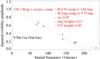 |
Fig. 8 Average of squared visibility amplitudes taken across the Na i line at 2.202–2.207 μm for V766 Cen as a function of spatial frequency. The red lines indicate the best-fit UD+ring+over-resolved component model (see text). |
Figure 8 shows the extracted average visibilities in the Na i line using the same bandwidth of 2.202–2.207 μm. Using the Na i ring diameter as the only remaining free parameter, we obtained a ring diameter of 5.77 mas, corresponding to about 1.5 times the photospheric continuum diameter. This model fit is shown together with the observed visibilities.
The closure phase signal of ~5 deg at the position of the Na i doublet relative to the nearby continuum corresponds to a photocenter displacement of the Na i ring with respect to the stellar continuum emission of ~0.16 mas. Here we use the formula for marginally resolved targets p = −Φ/2π × λ/B (Lachaume 2003; Le Bouquin et al. 2009), where p is the photocenter displacement and Φ is the phase signal.
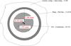 |
Fig. 9 Sketch of V766 Cen’s UD+ring+over-resolved component model for the emission at the wavelength of the Na i doublet. |
Fundamental properties of V766 Cen, σ Oph, BM Sco, and HD 206859.
For illustration, Fig. 9 shows a sketch of the contributing components of our toy model at the wavelength of the Na i doublet, including the continuum emission of the central star (UD component), the Na i emission from an offset ring-like component, and continuum emission from an over-resolved dust component. In addition, V766 Cen also shows extended CO emission, but that is not visible at this wavelength. The offset position of the Na i ring in the sketch represents the photocenter displacement between the Na i emission and the nearby continuum emission. It might be caused by effects of the nearby companion. It may also be possible to explain this displacement via convection patterns on the stellar surface that cause the photocenter of the stellar continuum to be different from the geometric center while the Na i emission is symmetric with respect to the outer radius of the star.
4. Fundamental stellar parameters and statistical properties
Properties of our sample of cool supergiants and giants.
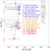 |
Fig. 10 Location of our updated sample of sources in the HR diagram (cf. Table 4). Also shown are evolutionary tracks from Ekström et al. (2012) for masses of 3–60 M⊙. The solid lines indicate models without rotation, and the dashed lines with rotation. Blue indicates the luminosity class I supergiants; orange indicates the transition region between giants and supergiants; and red indicates the luminosity class III red giants. |
Table 3 lists the fundamental parameters of our new sources based on our fits of the Rosseland angular diameters, the adopted bolometric fluxes and distances, and the evolutionary tracks by Ekström et al. (2012). Figure 10 shows the position of our new sources in the Hertzsprung-Russell (HR diagram) together with our previously observed sources from Wittkowski et al. (2012), Arroyo-Torres et al. (2013), and Arroyo-Torres et al. (2014), all of which were analyzed in the same way. This figure also shows the evolutionary tracks by Ekström et al. (2012) for initial masses between 3 M⊙ and 60 M⊙ with and without rotation. Our sample includes supergiants and giants, where the giants are non-Mira semi-regular or irregular variables.
4.1. Fundamental parameters of our new sources
The individual new sources are discussed in more detail in Sect. 5 below. In short, V766 Cen is found to be a high-luminosity star of log L/L⊙ ~ 5.8 ± 0.4, a radius of 1490 R⊙ ± 540 R⊙, and an effective temperature of ~4300 K ± 760 K. Its position in the HR diagram is close to the red edge of evolutionary tracks of initial mass 25–40 M⊙. BM Sco, σ Oph, and HD 206859 show luminosities log L/L⊙ ~ 3.35−3.55 corresponding to evolutionary tracks of initial masses 5–9 M⊙. The stars σ Oph and BM Sco are close to the red edge of these tracks with effective temperatures of 4130 ± 566 K and 3890 ±310 K, respectively, while HD 206859 is a warmer star of effective temperature 5250 ± 740 K.
4.2. Statistical properties of our sample
Table 4 lists the fundamental parameters of our full sample of 16 sources, i.e., those shown in the HR diagram in Fig. 10. It includes the luminosity class from Simbad, the luminosity, effective temperature, and radius from our calculations, the initial mass from our position in the HR diagram and the evolutionary tracks by Ekström et al. (2012), and the variability period from the GCVS (Samus et al. 2009) and the AAVSO database. The period of VY CMa is from Kiss et al. (2006). The table also includes the flux fraction A of the stellar component, i.e., a value of A< 1 indicates an additional over-resolved, possibly dusty, background component of flux fraction. Finally, we list whether or not we found an extended atmosphere beyond that predicted by 1D and 3D model atmospheres; cf. Arroyo-Torres et al. (2015).
Comparison to literature values.
In general, our results confirm the conclusion by Levesque et al. (2005) that the positions of RSGs in the HR diagram are consistent with the red edges of the evolutionary tracks near the Hayashi line. In particular, we have four sources in common with Levesque et al. (2005): HD 95687, HD 97671 (=V602 Car), HD 160371 (=BM Sco), and KW Sgr. We also have two sources in common with van Belle et al. (2009): HD 183589 and HD 206859. Table 5 provides the comparisons of the effective temperatures, luminosities, and absolute radii with our values. They are all consistent within 1σ, except for KW Sgr, for which Levesque et al. (2005) found a higher luminosity and a larger radius at the 2–3σ level. Our effective temperatures and luminosities of σ Oph, BM Sco, and HD 206859 are consistent with the estimates by McDonald et al. (2012) as well, except for the luminosity of BM Sco, where McDonald et al. (2012) found a lower value of log L/L⊙ = 3.0 compared to our value of log L/L⊙ = 3.5 ± 0.3.
Table 4 is ordered by decreasing luminosity. Our values confirm decreasing radius, initial mass, and pulsation period with decreasing luminosity, giving additional confidence in the consistency of our values. The outliers are VY CMa, which has an unusually long period, and UY Sct, which has an unusually large radius. The reasons for these outliers are not yet clear.
Our sources can be separated into three groups: (I) Sources of luminosity log L/L⊙ between about 5.8 and 4.8, which are consistently classified as luminosity class I sources. They correspond to initial masses between about 60 M⊙ and 12 M⊙. These are clearly supergiants. (II) Sources of log L/L⊙ between about 3.8 and 3.4, of which some are classified as luminosity class Ib and some as (II-)III. Some of these sources have conflicting classifications in the literature. They correspond to initial masses between 12 M⊙ and 5 M⊙. These sources may represent a transitional region between giants and supergiants. (III) Sources of luminosity log L/L⊙ below about 3.4, which are consistently classified as luminosity class III sources, corresponding to initial masses below about 7 M⊙. These are clearly giant stars. The groups are indicated by different colors in Fig. 10 (HR diagram) and Fig. 11 (effective temperature scale, discussed below).
An extended atmosphere, beyond the predictions by 1D and 3D model atmospheres, is seen only for the clear RSG sources (group I above) including the warmer source V766 Cen. Similarly, a significant contribution of a very extended over-resolved (dust) component is only seen for the most luminous RSG sources. BM Sco as a transitional source represents an exception and possibly shows a weak extension of the atmosphere and a strong contribution by an over-resolved component. The latter is consistent with McDonald et al. (2012), who list BM Sco as one of a few giants with an infrared flux excess indicating circumstellar material. This is unusual for a non-Mira giant of this luminosity. The cause of these effects is not clear; they might might possibly be due to an unseen binary companion.
Our sampling of luminosities presents an unsampled locus in the HR diagram around log L/L⊙ 3.8–4.8, corresponding to initial masses around 10–13 M⊙. Other well-known RSGs, including Betelgeuse, VX Sgr (cf. Arroyo-Torres et al. 2013), Antares (Ohnaka et al. 2013), and μ Cep (Perrin et al. 2005), which are not a part of our sample, have luminosities above log L/L⊙ ~ 4.8 as well. This gap appeared very naturally in our sampling, which was based on sources from the GCVS (Samus et al. 2009), which were classified as luminosity classes I–III and cool spectral types of K–M (with an emphasis in Lum. class I) and well observable with the VLTI/AMBER instrument in terms of brightness and expected angular size. It is not yet clear whether this gap is caused by a selection bias, or whether it may indicate a shorter lifetime of sources of this mass near the red edge of the evolutionary tracks. Possibly, stars below this mass range are (super)-AGB stars and return to warmer effective temperatures toward becoming planetary nebulae and stars above this mass range return to warmer effective temperatures toward becoming yellow supergiants and WR stars, while stars of this mass range explode as core-collapse SNe at the RSG stage. This may explain a shorter lifetime of these sources near the red edge of the evolutionary tracks. Such a scheme is roughly consistent with the evolutionary tracks of Ekström et al. (2012), where RSGs with initial masses larger than about 15⊙ start to return to warmer effective temperatures. Interestingly this range of masses corresponds to about that of some recently confirmed RSG progenitors of SNe of type II-P (Maund et al. 2014b,a, 2015), while for instance the higher mass (40 M⊙) progenitor of SN type Ic was found to be a yellow supergiant, i.e., it had not already exploded at the RSG stage (Maund & Ramirez-Ruiz 2016). Likewise, Smartt (2015) recently pointed out the deficit of high-mass stars (larger than 18 M⊙) among the progenitors of mostly II-P, II-L, or IIb core collapse SNe.
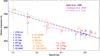 |
Fig. 11 Effective temperature vs. spectral type of our sources together with calibrations of the effective temperature scale by Dyck et al. (1998), Levesque et al. (2005), and van Belle et al. (2009). Blue indicates the luminosity class I supergiants; orange indicates the transition region between giants and supergiants; and red represents the luminosity class III red giants. |
4.3. Effective temperature scale
Figure 11 shows the effective temperature versus spectral type for our sample, together with empirical calibrations by Dyck et al. (1998) for cool giants stars, by van Belle et al. (2009) for cool giants stars and RSG stars, and by Levesque et al. (2005) for RSGs. Our data points are consistent with all of these calibrations within the error bars. In particular we are not yet able to prove or disprove a different effective temperature scale for supergiants and giants as suggested by Levesque et al. (2005).
4.4. Atmospheric extension
Arroyo-Torres et al. (2015) found a linear relation for RSGs (i.e., group I above) between the contribution by extended atmospheric CO layers, as measured by the squared visibility in the CO(2–0) bandhead relative to the nearby continuum, and the luminosity. This may support a scenario of radiative acceleration on molecules as a missing driver for the atmospheric extension of RSGs as suggested by Josselin & Plez (2007). Figure 12 shows the same relation as in Arroyo-Torres et al. (2015), but now also including our new supergiant source V766 Cen. As in Arroyo-Torres et al. (2015), we limited the calculation to continuum squared visibilities between 0.2 and 0.4, which is a range where the source is resolved and the visibility function is nearly linear. Interestingly, this relation is confirmed up to the location of V766 Cen, now extending to twice the previous luminosity range. This supports once again a similar mass loss mechanism of all RSGs over about an order of magnitude in luminosity. We note that V766 Cen has a luminosity (log L/L⊙ ~ 5.8) close to the Eddington luminosity (log L/L⊙ ~ 5.6–6.1 for masses 13–36 M⊙), above which stars become unstable owing to strong radiative winds. This may further support a scenario of steadily increasing radiative winds, and thus increasing magnitude of extended molecular layers with increasing luminosity.
The visibility drops discussed above indicate that CO is formed above the continuum-forming layers. The visibility ratios provide an estimate of the total contribution of the extended layers compared to the stellar continuum layers and not necessarily the ratio of the radii of these layers. We are not able to directly constrain the radii of the CO layers by our few snapshot observations owing to the unknown complex intensity profiles of CO (cf. Wittkowski et al. 2016, Fig. 3) and the lack of a satisfactory geometrical model to describe them. However, from comparisons of model atmospheres of AGB stars that predict extended layers and show similar visibility drops (e.g., Wittkowski et al. 2016), we can estimate that CO layers of RSG stars have comparable typical extensions of about 1.5–2 stellar radii. This puts the CO emission of V766 Cen at a similar radius as the Na i emission.
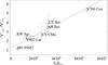 |
Fig. 12 Atmospheric extension vs. luminosity of our RSGs. The contribution by extended atmospheric CO layers is measured by ratio between the squared visibility amplitude in the continuum (average between 2.27 and 2.28 μm) and the squared visibility amplitude in the CO (2–0) line at 2.29 μm. The dashed gray line shows a linear fit to the data points. |
5. Discussion of individual sources
5.1. V766 Cen
V766 Cen (=HR 5171 A) was classified and discussed as a yellow hypergiant (YHG) by, for example, Humphreys et al. (1971), van Genderen (1992), de Jager (1998), and van Genderen et al. 2015. Chesneau et al. (2014) suggested that it has a very close, possibly common-envelope companion, which we took into account in our analysis. This classification implies that the star has a high luminosity and is located in the HR diagram between the blue and red parts of its evolutionary tracks, either evolving from the RSG phase back toward higher effective temperatures, or –less likely– from the main sequence toward the RSG phase.
Our results confirm that V766 Cen is a high-luminosity star. However, its effective temperature compared to the evolutionary tracks by Ekström et al. (2012) indicate that it is located close to the red edge of its evolutionary track and close to the Hayashi line, thus resembling a luminous RSG rather than a typical YHG. It may have a higher effective temperature compared to a more typical RSG, such as our other RSGs, simply because the Hayashi line shifts slightly to the left in the HR diagram for increasing mass (∂log Teff/∂log M ~ 0.2; see Kippenhahn & Weigert 1990). For example, this would move the Hayashi line from an effective temperature of 3500 K to 4300 K between stars of current mass 10 M⊙ and 30 M⊙. Details depend on metallicity and rotation. Figure 13 shows the effective temperature (top) and luminosity (bottom) as a function of current mass based on the tracks by Ekström et al. (2012) for solar metallicity with and without rotation. Also indicated are our values for V766 Cen with their errors. It illustrates that only those tracks of initial mass 40 M⊙ without rotation, 32 M⊙ without rotation, and (marginally) 25 M⊙ with rotation are consistent with our observations, corresponding to current masses of about 27–36 M⊙, 22–29 M⊙, 13–23 M⊙, respectively. The other tracks either do not decrease to our effective temperature or do not increase to our luminosity. Here, the track of 40 M⊙ without rotation is consistent with our values. A current mass of 27–36 M⊙ is also consistent with the current system mass estimated by Chesneau et al. (2014) of  M⊙ based on their NIGHTFALL models. The upper panel of Fig. 13 also illustrates nicely that V766 Cen is located close to the coolest part of its evolutionary track. The comparison of the position of V766 Cen in the HR diagram may be complicated by effects of the companion on its stellar evolution. Nevertheless, the position in the HR diagram itself is independent of the comparison to evolutionary tracks.
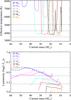 |
Fig. 13 Evolutionary status of V766 Cen. Effective temperature (top) and luminosity (bottom) as a function of mass during the evolution of 25 M⊙ to 80 M⊙ ZAMS evolutionary tracks from Ekström et al. (2012). The solid lines denote tracks without rotation and the dashed lines tracks with rotation. The horizontal lines denote our measurement of the effective temperature and luminosity of V766 Cen together with the error ranges. |
Chesneau et al. (2014) already noted that the radius of V766 Cen is unusually large for a typical YHG. Indeed, it is more consistent with an evolutionary status of a RSG with a fully convective envelope that is close to the Hayashi limit, as discussed above.
Our data of V766 Cen indicate a shell of Na i with a radius of 1.5 photospheric radii. Our closure phases indicate a small photocenter displacement of the Na i shell with respect to the stellar continuum of ~0.16 mas (8% of the photospheric radius). This displacement might possibly be caused by the presence of the close companion. Gorlova et al. (2006) and Oudmaijer & de Wit (2013) have described such shells around cool very luminous supergiants as due to a quasi-chromosphere or a steady shock wave at the interface of a fast expanding wind shielding the gas from direct starlight. The luminosity of log L/L⊙ ~ 5.8 ± 0.4 is close to the Eddington luminosity of log L/L⊙ ~ 5.6–6.1 for current masses of 13–36 M⊙, so that indeed strong radiative winds can be expected. The high luminosity compared to the Eddington luminosity also points toward the upper current mass range of V766 Cen discussed above.
V766 Cen shows extended molecular CO layers similar to the other RSGs of our sample. Arroyo-Torres et al. (2015) showed that the extension of these layers cannot be explained by current pulsation or convection models and that additional physical mechanisms are needed to explain them. We confirmed that the relation of increasing contribution by extended CO layers with increasing luminosity (Arroyo-Torres et al. 2015) extends to the luminosity of V766 Cen, which is close to the Eddington limit.
Finally, our data show evidence of an over-resolved (i.e., uncorrelated) background flux, which is consistent with a known silicate dust shell (Humphreys et al. 1971) that vastly exceeds our interferometric field of view, which is about 270 mas.
In summary, V766 is located close to both the Hayashi limit toward cooler effective temperatures and the Eddington limit toward higher luminosities. This source shows properties of RSGs, such as a relatively large radius and an extended molecular layer. It also shows properties of high-luminosity stars, such as a spatially extended shell of neutral sodium at about 1.5 stellar radii. The inner dust shell radius is not yet constrained. Verhoelst et al. (2006) suggested an inner dust shell of Al2O3 as close as 1.5 stellar radii for the RSG α Ori, which is consistent with most recent models (Gobrecht et al. 2016; Höfner et al. 2016) and observations (Ireland et al. 2005; Wittkowski et al. 2007; Norris et al. 2012; Karovicova et al. 2013) of AGB stars. If this is confirmed, it would put the Na i emission, the extended molecular (CO) layer, and inner dust formation zone at a similar radius of about 1.5 stellar radii, forming an optically thick region (aka pseudo-photosphere) at the onset of the wind.
5.2. BM Sco
BM Sco is generally classified as a K1-2.5 Ib supergiant (Simbad adopted K2 Ib). However, our luminosity of log L/L⊙ = 3.5 ± 0.3 places this source into a transitional zone between red giants and RSGs corresponding to evolutionary tracks of initial mass 5–9 M⊙. McDonald et al. (2012) placed this souces at an even lower luminosity of log L/L⊙ = 3.0. This position in the HR diagram is more consistent with a classification as K3 III by Houk (1982). The measured effective temperature of 3890 ± 310 K is consistent with the spectral classification. BM Sco is also among the source of Levesque et al. (2005) and our fundamental properties are consistent with theirs. We have found a significant uncorrelated flux fraction of ~25% from an over-resolved component, most likely pointing to a large background dust shell. This is consistent with McDonald et al. (2012) who list BM Sco as one of relatively few giants with infrared excess and evidence for circumstellar material. BM Sco also shows extended CO features in the visibility that may be slightly beyond model predictions. These features are not typical for a star of this mass range, but would be more typical for a higher luminosity and thus higher mass star. This makes BM Sco an interesting target for follow-up observations. These features might be caused by an interaction with a close unseen companion. We can also not exclude that adopted values for the distance or for the calculation of the bolometric flux may be erroneous, and that BM Sco in fact is a higher luminosity and higher mass star.
5.3. σ Oph
The star σ Oph is classified as spectral type K2-5 and luminosity class II–III (Simbad adopted K2 III). We find a luminosity of log L/L⊙ = 3.4 ± 0.3 and an effective temperature of 4130 ± 570 K, placing it at a similar place as BM Sco in the HR diagram within the errors, again in a transitional zone between red giants and RSGs, corresponding to initial masses of 5–9 M⊙. Our luminosity and effective temperature are consistent with those of McDonald et al. (2012).
5.4. HD 206859
HD 206859 is generally classified as a G5 Ib supergiant. However, similar to BM Sco and σ Oph, we find that it lies in the transitional zone between giants and supergiants at a luminosity of log L/L⊙ = 3.4 ± 0.3 corresponding to tracks of initial mass 5–9 M⊙. We find that it has the highest effective temperature of our sample of 5270 ± 740 K, which is consistent with having the warmest spectral type of our sample of G5. Our fundamental parameters of HD 206859 are consistent with those by van Belle et al. (2009) and McDonald et al. (2012).
6. Summary and conclusions
We observed four late-type supergiants of spectral types G5 to K2.5 with the AMBER instrument in order to derive their fundamental parameters and study their atmospheric structure. These sources include V766 Cen (=HR 5171 A), σ Oph, BM Sco, and HD 206859. The new observations complement our previous observations of cooler, mostly M-type, giants and supergiants, increasing our full sample to 16 sources. We derived effective temperatures, luminosities, and absolute radii. The values are generally consistent with other estimates available in the literature.
V766 Cen was classified as a yellow hypergiant in the literature, and is thought to have most likely evolved from the red supergiant stage back toward larger effective temperatures. Chesneau et al. (2014) suggested a close, possibly common-envelope companion, which we took into account in our analysis. We derived a luminosity of log L/L⊙ = 5.8 ± 0.4, an effective temperature of 4290 ± 760 K, a radius of 1490 ± 540 R⊙, and a surface gravity log g ~ −0.3. Contrary to the classification as a yellow hypergiant, our observations indicate that V766 Cen is located at the red edge of a high-mass, most likely 40 M⊙ track, thus representing a high-luminosity fully convective red supergiant rather than a yellow hypergiant. This is supported by a relatively large radius, which would be unusual for a typical YHG, and by the observed presence of extended CO layers, which are typical for RSGs. V766 Cen is located close to both the Hayashi limit toward cooler effective temperatures and the Eddington limit toward higher luminosities. V766 Cen shows a K-band flux spectrum that exhibits CO lines and the Na i doublet. The CO lines are weaker in the flux spectrum compared to our previously observed RSGs, which is consistent with the earlier spectral type. However, the visibility spectra indicate a relatively strong extension of the CO forming layers. The closure phases indicate deviations from symmetry at the CO bandheads. Extended clumpy molecular layers, most importantly water and CO in the near-infrared, are typical for RSGs and were previously observed for other RSGs. Arroyo-Torres et al. (2015) showed that the observed molecular extensions of RSGs cannot be reproduced by 1D and 3D pulsation and convection models, a missing physical process may explain the inability to reproduce these observed molecular extensions. The Na i doublet toward V766 Cen is also spatially resolved. We estimated a shell radius of about 1.5 stellar photospheric radii. The closure and differential phases indicate a photocenter displacement of the Na i shell compared to the nearby continuum of about 0.1 RPhot. Lines of neutral sodium are typical for high-luminosity RSGs and hypergiants as discussed, for instance, by Gorlova et al. (2006) and Oudmaijer & de Wit (2013). These studies suggest that a dense quasi-chromosphere located just above the photosphere or an optically thick pseudo-photosphere formed by the wind shields the gas from direct starlight and prevents it from being ionized. Our observations suggest that the extended molecular atmosphere and the Na i shell may coincide and represent an optically thick region at the onset of the wind. The photocenter displacement between the Na i line and the continuum may be caused by the effects of the close companion on the nearby circumstellar environment or by asymmetric convection patterns on the continuum-forming surface of the star.
We found luminosities log L/L⊙ for BM Sco, σ Oph, and HD 206859 of 3.5 ± 0.3, 3.4 ± 0.3, 3.4 ± 0.3, effective temperatures of 3890 ± 310 K, 4130 ± 570 K, 5270 ± 740 K, Rosseland radii of 129 ± 26 R⊙, 100 ± 30 R⊙, 57 ± 17 R⊙, and surface gravities log g of about 1.1, 1.3, and 1.8, respectively. These sources show CO features in the flux spectra, but with visibility spectra indicating that CO is formed at photospheric layers. There is no indication of extended molecular layers for these sources. Compared to evolutionary tracks, they correspond to initial masses of 5 M⊙ and 9 M⊙. Altogether, despite their classification as luminosity class Ib sources, they more likely represent higher mass giants than supergiants. BM Sco exhibits a significant flux fraction of about 25% from an underlying over-resolved dusty background component, which is consistent with an earlier indication of circumstellar material (McDonald et al. 2012). This is unusual among our sources of this mass, which makes BM Sco an interesting target for follow-up observations.
The relatively low luminosities of the luminosity class Ib sources of our sample leaves us with an unsampled locus in the HR diagram corresponding to luminosities log L/L⊙ ~ 3.8–4.8 or masses 10–13 M⊙. This region might correspond to evolutionary tracks where RSGs explode as core-collapse (type II-P) SN, while stars of lower and higher masses return to higher effective temperatures. In fact, this mass range corresponds to about the mass range of recently confirmed red supergiant progenitors of type II-P SN. It will be of interest for upcoming observations to find RSGs of this luminosity range to determine whether the gap is due to a selection effect or a lower probability of finding RSGs of these luminosities.
The previously found relation of increasing strength of extended molecular layers with increasing luminosity (Arroyo-Torres et al. 2015) was now confirmed to extend to the luminosity of V766 Cen. This represents twice the previous luminosity range and now reaches a level near the Eddington limit. This might further point to steadily increasing radiative winds with increasing luminosity as a possible explanation for the observed extensions of atmospheric molecular layers toward RSGs.
See AMBER Data Reduction Software User Manual; http://www.jmmc.fr/doc/approved/JMMC-MAN-2720-0001.pdf
Best-fit model 1 of their Table 2.
Acknowledgments
We thank Antxon Alberdi for scientific discussions during the data reduction. This research has made use of the AMBER data reduction package of the Jean-Marie Mariotti Center. This research has made use of the SIMBAD database, operated at CDS, France. This research has made use of NASA’s Astrophysics Data System. We acknowledge with thanks the variable star observations from the AAVSO International Database contributed by observers worldwide and used in this research.
References
- Anderson, E., & Francis, C. 2012, Astron. Lett., 38, 331 [NASA ADS] [CrossRef] [Google Scholar]
- Arroyo-Torres, B., Wittkowski, M., Marcaide, J. M., & Hauschildt, P. H. 2013, A&A, 554, A76 [NASA ADS] [CrossRef] [EDP Sciences] [Google Scholar]
- Arroyo-Torres, B., Martí-Vidal, I., Marcaide, J. M., et al. 2014, A&A, 566, A88 [NASA ADS] [CrossRef] [EDP Sciences] [Google Scholar]
- Arroyo-Torres, B., Wittkowski, M., Chiavassa, A., et al. 2015, A&A, 575, A50 [NASA ADS] [CrossRef] [EDP Sciences] [Google Scholar]
- Beichman, C. A., Neugebauer, G., Habing, H. J., Clegg, P. E., & Chester, T. J. 1988, Infrared astronomical satellite (IRAS) catalogs and atlases, Explanatory supplement, 1 [Google Scholar]
- Chelli, A., Utrera, O. H., & Duvert, G. 2009, A&A, 502, 705 [NASA ADS] [CrossRef] [EDP Sciences] [Google Scholar]
- Chesneau, O., Meilland, A., Chapellier, E., et al. 2014, A&A, 563, A71 [NASA ADS] [CrossRef] [EDP Sciences] [Google Scholar]
- Cutri, R. M., Skrutskie, M. F., van Dyk, S., et al. 2003, VizieR Online Data Catalog: II/246 [Google Scholar]
- de Jager, C. 1998, A&ARv, 8, 145 [NASA ADS] [CrossRef] [Google Scholar]
- de Wit, W. J., Oudmaijer, R. D., Fujiyoshi, T., et al. 2008, ApJ, 685, L75 [NASA ADS] [CrossRef] [Google Scholar]
- Dessart, L., Hillier, D. J., Waldman, R., & Livne, E. 2013, MNRAS, 433, 1745 [NASA ADS] [CrossRef] [Google Scholar]
- Ducati, J. R., Bevilacqua, C. M., Rembold, S. B., & Ribeiro, D. 2001, ApJ, 558, 309 [NASA ADS] [CrossRef] [Google Scholar]
- Dyck, H. M., van Belle, G. T., & Thompson, R. R. 1998, AJ, 116, 981 [NASA ADS] [CrossRef] [Google Scholar]
- Ekström, S., Georgy, C., Eggenberger, P., et al. 2012, A&A, 537, A146 [NASA ADS] [CrossRef] [EDP Sciences] [Google Scholar]
- Gobrecht, D., Cherchneff, I., Sarangi, A., Plane, J. M. C., & Bromley, S. T. 2016, A&A, 585, A6 [NASA ADS] [CrossRef] [EDP Sciences] [Google Scholar]
- Gorlova, N., Lobel, A., Burgasser, A. J., et al. 2006, ApJ, 651, 1130 [NASA ADS] [CrossRef] [Google Scholar]
- Groh, J. H., Meynet, G., Georgy, C., & Ekström, S. 2013, A&A, 558, A131 [NASA ADS] [CrossRef] [EDP Sciences] [Google Scholar]
- Hauschildt, P. H., Allard, F., Ferguson, J., Baron, E., & Alexander, D. R. 1999, ApJ, 525, 871 [NASA ADS] [CrossRef] [Google Scholar]
- Heger, A., Fryer, C. L., Woosley, S. E., Langer, N., & Hartmann, D. H. 2003, ApJ, 591, 288 [NASA ADS] [CrossRef] [Google Scholar]
- Höfner, S., Bladh, S., Aringer, B., & Ahuja, R. 2016, A&A, 594, A108 [NASA ADS] [CrossRef] [EDP Sciences] [Google Scholar]
- Houk, N. 1982, Michigan Catalogue of Two-dimensional Spectral Types for the HD stars, Vol. 3, Declinations –40deg to –26deg (University of Michigan Publ.) [Google Scholar]
- Humphreys, R. M. 1978, ApJS, 38, 309 [NASA ADS] [CrossRef] [EDP Sciences] [Google Scholar]
- Humphreys, R. M., Strecker, D. W., & Ney, E. P. 1971, ApJ, 167, L35 [NASA ADS] [CrossRef] [Google Scholar]
- Ireland, M. J., Tuthill, P. G., Davis, J., & Tango, W. 2005, MNRAS, 361, 337 [NASA ADS] [CrossRef] [Google Scholar]
- Josselin, E., & Plez, B. 2007, A&A, 469, 671 [NASA ADS] [CrossRef] [EDP Sciences] [Google Scholar]
- Karovicova, I., Wittkowski, M., Ohnaka, K., et al. 2013, A&A, 560, A75 [NASA ADS] [CrossRef] [EDP Sciences] [Google Scholar]
- Kharchenko, N. V. 2001, Kinematika i Fizika Nebesnykh Tel, 17, 409 [NASA ADS] [Google Scholar]
- Kippenhahn, R., & Weigert, A. 1990, Stellar Structure and Evolution (Berlin, Heidelberg, New York: Springer-Verlag) [Google Scholar]
- Kiss, L. L., Szabó, G. M., & Bedding, T. R. 2006, MNRAS, 372, 1721 [Google Scholar]
- Lachaume, R. 2003, A&A, 400, 795 [NASA ADS] [CrossRef] [EDP Sciences] [Google Scholar]
- Lafrasse, S., Mella, G., Bonneau, D., et al. 2010, VizieR Online Data Catalog: II/300 [Google Scholar]
- Lançon, A., & Wood, P. R. 2000, A&AS, 146, 217 [NASA ADS] [CrossRef] [EDP Sciences] [Google Scholar]
- LeBouquin, J.-B., Absil, O., Benisty, M., et al. 2009, A&A, 498, L41 [NASA ADS] [CrossRef] [EDP Sciences] [Google Scholar]
- Levesque, E. M., Massey, P., Olsen, K. A. G., et al. 2005, ApJ, 628, 973 [NASA ADS] [CrossRef] [Google Scholar]
- Maund, J. R., & Ramirez-Ruiz, E. 2016, MNRAS, 456, 3175 [NASA ADS] [CrossRef] [Google Scholar]
- Maund, J. R., Mattila, S., Ramirez-Ruiz, E., & Eldridge, J. J. 2014a, MNRAS, 438, 1577 [NASA ADS] [CrossRef] [Google Scholar]
- Maund, J. R., Reilly, E., & Mattila, S. 2014b, MNRAS, 438, 938 [NASA ADS] [CrossRef] [Google Scholar]
- Maund, J. R., Fraser, M., Reilly, E., Ergon, M., & Mattila, S. 2015, MNRAS, 447, 3207 [NASA ADS] [CrossRef] [Google Scholar]
- McDonald, I., Zijlstra, A. A., & Boyer, M. L. 2012, MNRAS, 427, 343 [NASA ADS] [CrossRef] [Google Scholar]
- Mermilliod, J.-C., & Paunzen, E. 2003, A&A, 410, 511 [NASA ADS] [CrossRef] [EDP Sciences] [Google Scholar]
- Meynet, G., Chomienne, V., Ekström, S., et al. 2015, A&A, 575, A60 [NASA ADS] [CrossRef] [EDP Sciences] [Google Scholar]
- Moshir, M., et al. 1990, in IRAS Faint Source Catalogue, version 2.0 [Google Scholar]
- Norris, B. R. M., Tuthill, P. G., Ireland, M. J., et al. 2012, Nature, 484, 220 [NASA ADS] [CrossRef] [PubMed] [Google Scholar]
- Ohnaka, K., Hofmann, K.-H., Schertl, D., et al. 2013, A&A, 555, A24 [NASA ADS] [CrossRef] [EDP Sciences] [Google Scholar]
- Oudmaijer, R. D., & de Wit, W. J. 2013, A&A, 551, A69 [NASA ADS] [CrossRef] [EDP Sciences] [Google Scholar]
- Perrin, G., Ridgway, S. T., Mennesson, B., et al. 2004, A&A, 426, 279 [NASA ADS] [CrossRef] [EDP Sciences] [Google Scholar]
- Perrin, G., Ridgway, S. T., Verhoelst, T., et al. 2005, A&A, 436, 317 [NASA ADS] [CrossRef] [EDP Sciences] [Google Scholar]
- Petrov, R. G., Malbet, F., Weigelt, G., et al. 2007, A&A, 464, 1 [NASA ADS] [CrossRef] [EDP Sciences] [Google Scholar]
- Samus, N. N., Durlevich, O. V., et al. 2009, VizieR Online Data Catalog: B/gcvs [Google Scholar]
- Schlafly, E. F., & Finkbeiner, D. P. 2011, ApJ, 737, 103 [NASA ADS] [CrossRef] [Google Scholar]
- Smartt, S. J. 2015, PASA, 32, e016 [NASA ADS] [CrossRef] [Google Scholar]
- Smith, N. 2014, ARA&A, 52, 487 [NASA ADS] [CrossRef] [MathSciNet] [Google Scholar]
- Smith, N., Hinkle, K. H., & Ryde, N. 2009, AJ, 137, 3558 [NASA ADS] [CrossRef] [Google Scholar]
- Tatulli, E., Millour, F., Chelli, A., et al. 2007, A&A, 464, 29 [NASA ADS] [CrossRef] [EDP Sciences] [Google Scholar]
- van Belle, G. T., Creech-Eakman, M. J., & Hart, A. 2009, MNRAS, 394, 1925 [NASA ADS] [CrossRef] [Google Scholar]
- van Genderen, A. M. 1992, A&A, 257, 177 [NASA ADS] [Google Scholar]
- van Genderen, A. M., Nieuwenhuijzen, H., & Lobel, A. 2015, A&A, 583, A98 [NASA ADS] [CrossRef] [EDP Sciences] [Google Scholar]
- Verhoelst, T., Decin, L., van Malderen, R., et al. 2006, A&A, 447, 311 [NASA ADS] [CrossRef] [EDP Sciences] [Google Scholar]
- Verhoelst, T., van der Zypen, N., Hony, S., et al. 2009, A&A, 498, 127 [NASA ADS] [CrossRef] [EDP Sciences] [Google Scholar]
- Walmswell, J. J., & Eldridge, J. J. 2012, MNRAS, 419, 2054 [NASA ADS] [CrossRef] [Google Scholar]
- Warren, P. R. 1973, MNRAS, 161, 427 [NASA ADS] [Google Scholar]
- Wittkowski, M., Boboltz, D. A., Ohnaka, K., Driebe, T., & Scholz, M. 2007, A&A, 470, 191 [NASA ADS] [CrossRef] [EDP Sciences] [Google Scholar]
- Wittkowski, M., Hauschildt, P. H., Arroyo-Torres, B., & Marcaide, J. M. 2012, A&A, 540, L12 [NASA ADS] [CrossRef] [EDP Sciences] [Google Scholar]
- Wittkowski, M., Chiavassa, A., Freytag, B., et al. 2016, A&A, 587, A12 [NASA ADS] [CrossRef] [EDP Sciences] [Google Scholar]
- Yoon, S.-C., & Cantiello, M. 2010, ApJ, 717, L62 [NASA ADS] [CrossRef] [Google Scholar]
Appendix A: Additional figure
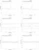 |
Fig. A.1 Left: observed normalized flux, squared visibility amplitudes, and closure phases (from top to bottom) around the Na i line of V766 Cen obtained with the MR-K 2.1 μm setting. Right: same as left but obtained with the MR-K 2.3 μm. |
All Tables
All Figures
|
Fig. 1 Left (from top to bottom): observed (black) normalized flux, squared visibility amplitudes, and closure phases of V766 Cen obtained with the MR-K 2.1 μm setting on 2014 April 07. Right: same as left but obtained with the MR-K 2.3 μm setting on 2014 April 07. The black solid lines connect all the observed data points, while for the sake of clarity, the “X” symbols and associated error bars are shown for only every fifth data point. The blue curves show the best-fit UD model, and the red curves the best-fit PHOENIX model prediction. The visibility plots (middle panels) show three curves, one for each of the three baselines of the AMBER triangle. (cf. Sect. 3.2). |
| In the text | |
|
Fig. 2 As Fig. 1, but for data of σ Oph obtained with the MR-K 2.1 μm setting on 2014 April 25 (left) and with the MR-K 2.3 μm setting on 2014 April 07 (right). |
| In the text | |
|
Fig. 3 As Fig. 1, but for data of BM Sco obtained with the MR-K 2.1 μm setting on 2014 April 25 (left) and with the MR-K 2.3 μm setting on 2014 April 07 (right). |
| In the text | |
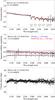 |
Fig. 4 As Fig. 1, but for data of BM Sco obtained with the MR-K 2.3 μm setting on 2014 June 09. |
| In the text | |
|
Fig. 5 As Fig. 1, but for data of HD 206859 obtained with the MR-K 2.1 μm setting on 2014 June 20 (left) and with the MR-K 2.3 μm setting on 2014 June 25 (right). |
| In the text | |
|
Fig. 6 Average of squared visibility amplitudes taken in the near-continuum bandpass at 2.05–2.20 μm for (from top to bottom) V766 Cen, σ Oph, BM Sco, and HD 206859 as a function of spatial frequency. The red lines indicate the best-fit UD models and the blue lines the best-fit PHOENIX models. The dashed lines are the maximum and minimum visibility curves, from which we estimated the errors of the angular diameters. |
| In the text | |
|
Fig. 7 Influence of the close companion of V766 Cen on the visibility curve. The asterisk and diamond symbols denote our near-continuum (2.05–2.20 μm) data, the central dashed line denotes the best-fit UD with over-resolved component, and the dash-dotted lines the error of the UD diameter. The color curves show the synthetic visibilities of a binary toy model consisting of two UDs and an over-resolved component with flux ratios as derived by Chesneau et al. (2014). The different colors indicate different positions of the companion corresponding along the projected orbit. The figure illustrates that our observations cannot separate between these curves and thus cannot fully characterize the companion. The range of the visibility curves of our binary toy model are within our already adopted diameter error. |
| In the text | |
|
Fig. 8 Average of squared visibility amplitudes taken across the Na i line at 2.202–2.207 μm for V766 Cen as a function of spatial frequency. The red lines indicate the best-fit UD+ring+over-resolved component model (see text). |
| In the text | |
|
Fig. 9 Sketch of V766 Cen’s UD+ring+over-resolved component model for the emission at the wavelength of the Na i doublet. |
| In the text | |
|
Fig. 10 Location of our updated sample of sources in the HR diagram (cf. Table 4). Also shown are evolutionary tracks from Ekström et al. (2012) for masses of 3–60 M⊙. The solid lines indicate models without rotation, and the dashed lines with rotation. Blue indicates the luminosity class I supergiants; orange indicates the transition region between giants and supergiants; and red indicates the luminosity class III red giants. |
| In the text | |
|
Fig. 11 Effective temperature vs. spectral type of our sources together with calibrations of the effective temperature scale by Dyck et al. (1998), Levesque et al. (2005), and van Belle et al. (2009). Blue indicates the luminosity class I supergiants; orange indicates the transition region between giants and supergiants; and red represents the luminosity class III red giants. |
| In the text | |
|
Fig. 12 Atmospheric extension vs. luminosity of our RSGs. The contribution by extended atmospheric CO layers is measured by ratio between the squared visibility amplitude in the continuum (average between 2.27 and 2.28 μm) and the squared visibility amplitude in the CO (2–0) line at 2.29 μm. The dashed gray line shows a linear fit to the data points. |
| In the text | |
|
Fig. 13 Evolutionary status of V766 Cen. Effective temperature (top) and luminosity (bottom) as a function of mass during the evolution of 25 M⊙ to 80 M⊙ ZAMS evolutionary tracks from Ekström et al. (2012). The solid lines denote tracks without rotation and the dashed lines tracks with rotation. The horizontal lines denote our measurement of the effective temperature and luminosity of V766 Cen together with the error ranges. |
| In the text | |
|
Fig. A.1 Left: observed normalized flux, squared visibility amplitudes, and closure phases (from top to bottom) around the Na i line of V766 Cen obtained with the MR-K 2.1 μm setting. Right: same as left but obtained with the MR-K 2.3 μm. |
| In the text | |
Current usage metrics show cumulative count of Article Views (full-text article views including HTML views, PDF and ePub downloads, according to the available data) and Abstracts Views on Vision4Press platform.
Data correspond to usage on the plateform after 2015. The current usage metrics is available 48-96 hours after online publication and is updated daily on week days.
Initial download of the metrics may take a while.