| Issue |
A&A
Volume 597, January 2017
|
|
|---|---|---|
| Article Number | A12 | |
| Number of page(s) | 22 | |
| Section | Stellar structure and evolution | |
| DOI | https://doi.org/10.1051/0004-6361/201628979 | |
| Published online | 19 December 2016 | |
Unraveling the formation history of the black hole X-ray binary LMC X-3 from the zero age main sequence to the present⋆
1 Observatoire de Genève, University of Geneva, Route de Sauverny, 1290 Versoix, Switzerland
e-mail: mads.sorensen@unige.ch
2 MIT Kavli Institute for Astrophysics and Space Research, Cambridge, MA 02139, USA
3 Harvard-Smithsonian Center for Astrophysics, 60 Garden Street, Cambridge, MA 02138, USA
4 Center for Interdisciplinary Exploration and Research in Astrophysics (CIERA) and Department of Physics and Astrophysics, Northwestern University, Evanston, IL 60208, USA
Received: 21 May 2016
Accepted: 3 August 2016
Aims. We have endeavoured to understand the formation and evolution of the black hole (BH) X-ray binary LMC X-3. We estimated the properties of the system at four evolutionary stages: (1) at the zero-age main-sequence (ZAMS); (2) immediately before the supernova (SN) explosion of the primary; (3) immediately after the SN; and (4) at the moment when Roche-lobe overflow began.
Methods. We used a hybrid approach that combined detailed calculations of the stellar structure and binary evolution with approximate population synthesis models. This allowed us to estimate potential natal kicks and the evolution of the BH spin. We incorporated as model constraints the most up-to-date observational information throughout, which include the binary orbital properties, the companion star mass, effective temperature, surface gravity and radius, and the BH mass and spin.
Results. We find at 5% and 95% confidence, respectively, that LMC X-3 began as a ZAMS system with the mass of the primary star in the range M1,ZAMS = 22–31 M⊙ and a secondary star of M2,ZAMS = 5.0−8.3 M⊙, in a wide (PZAMS ≳ 2.000 days) and eccentric (eZAMS ≳ 0.18) orbit. Immediately before the SN, the primary had a mass of M1,preSN = 11.1−18.0 M⊙, but the secondary star was largely unaffected. The orbital period decreased to 0.6−1.7 days and is still eccentric 0 ≤ epreSN ≤ 0.44. We find that a symmetric SN explosion with no or small natal kicks (a few tens of km s-1) imparted on the BH cannot be formally excluded, but large natal kicks in excess of ≳120 km s-1 increase the estimated formation rate by an order of magnitude. Following the SN, the system has a BH MBH,postSN = 6.4−8.2 M⊙ and is set on an eccentric orbit. At the onset of the Roche-lobe overflow, the orbit is circular and has a period of PRLO = 0.8−1.4 days.
Key words: black hole physics / binaries: general / stars: black holes / stars: evolution / quasars: individual: LMC X-3 / X-rays: binaries
The full Table 2 is only available at the CDS via anonymous ftp to cdsarc.u-strasbg.fr (130.79.128.5) or via http://cdsarc.u-strasbg.fr/viz-bin/qcat?J/A+A/597/A12
© ESO, 2016
1. Introduction
X-ray binaries (XRBs) are evolved stellar binary systems containing a compact object (CO), a neutron star (NS) or a black hole (BH), and a companion star that is losing mass. The companion star, also known as the donor star, loses mass either because it is overflowing its Roche lobe or through stellar winds. A fraction of the lost mass is transferred to the CO that upon accretion emits X-rays, hence their name. In consequence of the mass transfer (MT), the orbital period of the system changes.
Roche-lobe overflow (RLO) is initiated either when the donor star expands as a result of the restructuring of its stellar interior, for instance, when the star leaves the main sequence (MS) and expands outside its Roche lobe, or because angular momentum loss processes (e.g., gravitational wave radiation and magnetic braking) shrink the orbit. RLO triggers MT through the first Lagrangian point directly into the potential well of the CO. Stellar winds, on the other hand, play a less dominant role in shrinking the orbit and are relevant mostly for XRBs with massive donors that are able to generate winds sufficiently powerful to cause a high mass loss, such as those observed in Wolf-Rayet stars or red giants (e.g. Nugis & Lamers 2000; van Loon et al. 2005). For hot stars, whose stellar winds are nearly spherically symmetric and fast, of ~1000 km s-1, Bondi-Hoyle accretion (Bondi 1952) of these stellar winds onto the CO is far less effective as a MT mechanism to power an XRB than RLO. However, fast-wind Bondi-Hoyle accretion affects not only the orbital separation of the binary, but may also enhance the system eccentricity for a mass ratio <0.78 (Dosopoulou & Kalogera 2016a,b).
Since their first discovery, BH XRBs have proven an essential natural laboratory for studying stellar BHs. These systems provide the best observational test for the existence of BHs that are formed from stellar collapse and the only type of systems where the properties of a stellar BH, that is, its mass and angular momentum, can be measured based on observations in the electromagnetic spectrum (Cowley 1992; Remillard & McClintock 2006; McClintock et al. 2013). Furthermore, they provide us with unique observational constraints for binary evolution and CO formation models.
The growing sample of Galactic and extragalactic BH XRBs instigated a number of studies about their formation. However, most of them either focused on the details of individual evolutionary phases or compared evolutionary models with only a subset of the available observational data (e.g., Lee et al. 2002; Belczynski & Bulik 2002; Podsiadlowski et al. 2002, 2003; Justham et al. 2006; Ivanova 2006; Brown et al. 2008; Fragos et al. 2010; Belczynski et al. 2011; Li 2015; Naoz et al. 2016, and references therein).
With our knowledge of the currently observed properties of an XRB system, it is in principle possible to reconstruct its evolution from the moment the system was comprised of two zero-age main-sequence (ZAMS) stars through the intermediate phases: primary to secondary MT, the common envelop (CE) phase, mass loss and kicks during the SN, including changes in the systems orbital characteristics, and concluding with the state of the system at the initiation of its current MT phase that causes its X-ray emission.
We define three groups of XRBs depending on the mass of the donor star. Low-mass XRBs (LMXBs) are systems with donor masses M2< 3 M⊙, high-mass XRBs (HMXBs) have donors more massive than M2 ≥ 10 M⊙, and intermediate-mass XRBs (IMXBs) are those XRBs with donor masses in the range 3 ≤ M2/M⊙< 10.
For the analysis of the Galactic LMXB GRO J1655-40, Willems et al. (2005) developed for the first time a method that combined all these aspects, including the modeling of the MT phase, the secular evolution of the binary before the RLO, the CO formation and core-collapse dynamics, and the motion of the system in the Galactic potential, into one comprehensive analysis. The results of this analysis were compared to all available observational constraints, including the three-dimensional position and velocity of the system in the Galaxy. Following a method similar to Willems et al. (2005), several systems have since been systematically analyzed (Fragos et al. 2009; Valsecchi et al. 2010; Wong et al. 2012, 2014).
One aspect of CO formation that has been recognized as an important element, but is not yet understood from first physical principles, concerns the effect of asymmetries associated with the core-collapse process and the resulting natal kicks imparted to NSs and BHs, which causes very high peculiar velocities, that is, the center-of-mass velocity relative to the local standard of rest. For NSs, kinematic observations of radio pulsar populations strongly suggest that NSs acquire very significant natal kicks of about a few to several hundreds of km s-1 (e.g., Hobbs et al. 2005). More recently, evidence from studies of binary systems of two NSs (e.g., Piran & Shaviv 2005; Willems et al. 2006) have indicated that there may be a subset of NSs that acquires significantly smaller kicks, of about tens of km s-1. A proposed explanation for these smaller kicks is that these NSs formed through an electron-capture SN instead of an Fe core-collapse (Podsiadlowski et al. 2004, 2005; Linden et al. 2009). Similarly, the Be/X-ray binaries (i.e., HMXBs with NS compact objects and Be-type star companions) in the two Magellanic Clouds show transverse velocities of up to a few tens of km s-1 (<15–20 km s-1; Antoniou et al. (2010), Antoniou & Zezas (2016) with LMC HMXBs traveling with velocities of up to four times higher than those of their SMC counterparts.
Our understanding of BH formation has evolved significantly in recent years, but compared to NSs, observational evidence of natal kicks is rare (Mirabel et al. 2001, 2002; Reid et al. 2014). Natal kicks are important because they are an indicator of the formation process of BHs. A large inferred natal kick (≳100 km s-1) is evidence of a core-collapse process accompanied by a SN explosion with asymmetric ejecta, while natal kicks of ~10 km s-1 indicate a symmetric supernova explosion with perhaps some asymmetries in the neutrino emission, or even BH formation through direct collapse. The BH in the Galactic LMXB XTE J1118+480 is currently the only BH for which an asymmetric natal kick, in the range 80–310 km s-1, has been inferred to not only be plausible but required to explain the formation of the system (Fragos et al. 2009). Willems et al. (2005) found that the BH in GRO J1655-40 most likely formed with a kick of up to 210 km s-1, which led to a kick of the system’s center-of-mass of 45–115 km s-1. However, a zero kick also provides a solution that is marginally consistent with the observed properties of the system. The system V404 Cyg also shows a high peculiar velocity, which suggests 47–102 km s-1 and indicates that this system also received a kick at BH formation, either from mass loss or during the SN (Miller-Jones et al. 2009a,b). Repetto et al. (2012) studied the Galactic population of LMXBs using analytical estimates of their evolutionary history and following the orbits of the systems in a Galactic potential, which showed that their large vertical spread relative to the Galactic plane could be explained by introducing a natal kick at the BH formation, and derived constraints on the possible kick imparted on the BH of each system in general agreement with previous studies of individual systems. Recently, Repetto & Nelemans (2015) followed up on their first study and argued that the seven LMXB system they considered received a natal asymmetric kick; five of these sources with relatively small kicks and two with kicks of several hundred km s-1. However, Mandel (2016) argued that this claim by Repetto & Nelemans (2015) is based on a problematic assumption of the likely direction of the kick and the Galactic dynamics of any LMXB born in the thin disk, suggesting that natal asymmetric kicks in excess of ~100 km s-1 are unlikely.
Studies of the evolutionary history of HMXBs have also been carried out. Valsecchi et al. (2010) studied the formation of the massive BH XRB M33 X-7 and found that an asymmetric kick was possibly imparted onto the BH during the core-collapse. However, such a kick is not required to explain the formation of the system. Wong et al. (2014) reached similar conclusions for IC10 X-1, concluding that the BH in this system cannot have received a kick larger than 130 km s-1, while the analysis of the evolutionary history of Cyg X-1 resulted in an upper limit for a potential asymmetric kick onto the BH of <77 km s-1 (Wong et al. 2012).
Over the past decade, measuring the spins of stellar-mass BHs became possible by three different methods: the thermal X-ray continuum fitting method, the iron Kα method, and the analysis of the quasi-periodic oscillations (QPOs) of the X-ray emission. For an extensive review of the different methods and the currently available measurements see McClintock et al. (2013), Reynolds (2013), Motta et al. (2014) and references therein. The measured values of the spin parameter a∗ for the different BHs cover the whole parameter space from a∗ = 0 (non-rotating BHs) all the way to a∗ = 1 (maximally rotating BHs), where a∗ ≡ cJ/GM2 with | a∗ | ≤ 1. Here M and J are the BH mass and angular momentum, respectively, c is the speed of light in vacuum, and G is the gravitational constant. The question naturally arises about the origin of the measured BH spin. Fragos & McClintock (2015) showed that the spin of known Galactic LMXBs can be explained by the mass accreted by the BH after its formation. This also implies that the natal BH masses in these systems are significantly different from those currently observed. In contrast, BHs in HMXBs have spins that cannot be explained through accretion after the BH formation because of their short lifetimes and relatively low mass-accretion rates. Hence their spin is most likely natal (Valsecchi et al. 2010; Gou et al. 2011). However, see also Moreno Méndez et al. (2008, 2011), Moreno Méndez (2011), who suggested that BH HMXB can obtain their spin after formation through a short period of extreme mass accretion, the so-called hypercritical accretion, which is orders of magnitudes higher than the critical Eddington accretion rate.
LMC X-3 is an intriguing accreting BH binary that stands out from the rest of the Roche-lobe overfilling dynamically confirmed BH XRBs. The donor star in LMC X-3 is a thermally disturbed star of early-B type, making it the most massive among the known Roche-lobe overfilling BH XRBs (Orosz et al. 2014). This classifies it as belonging to the elusive group of IMXBs. When the donor stars of IMXBs are losing mass, they quickly evolve to the significantly longer-lived phase of LMXBs. This naturally explains their overall rarity. The fact that we observe such a system in a small galaxy like the Large Magellanic Cloud (LMC) can be explained by the recent star-formation history of the LMC, see Sect. 4.4. Because it is a member of the LMC, it also has a very well determined distance. LMC X-3 has always been bright, albeit highly variable, in X-rays since the first X-ray telescope observed LMC back in the 1970s (Leong et al. 1971). This unusual behavior in its X-ray emission again sets LMC X-3 apart from other typical BH LMXBs (Steiner et al. 2014a). Therefore, it is important to place LMC X-3 within the frame of its relatives to see how this system has formed and evolved and to understand its current highly variable nature.
We investigate the past evolution of LMC X-3 from a ZAMS binary through intermediate phases until the current XRB phase. We follow the evolution of LMC X-3 using a hybrid approach, where we combine detailed calculations of the stellar structure and binary evolution with more approximate population synthesis calculation in an approach similar to that of Fragos et al. (2015). Using the stellar evolution code Modules for Experiments in Stellar Astrophysics (Paxton et al. 2011, 2013, 2015, MESA), we first scan a four-dimensional parameter space for potential progenitor systems (PPS) of LMC X-3 at the onset of RLO. We then continue with the parametric binary evolution code BSE (Hurley et al. 2000, 2002) to conduct a population synthesis study starting at the ZAMS and evolve a large set of binaries until the onset of RLO, matching the outcome of BSE with that of MESA to determine the PPS of LMC X-3 at the ZAMS. In doing so, we also estimate potential natal kicks and the evolution of the BH spin. We incorporate as model constraints the most up-to-date observational information of the system.
The layout of the paper is as follows. In Sect. 2 we consider the observational history and currently available observational constraints on the properties of LMC X-3. Section 3 describes how we modeled the current MT phase from RLO onset to the present and search a grid of MT sequence models to fit the observational constraints. We conclude Sect. 3 by presenting the result of MT sequences describing the LMC X-3 at the onset of RLO. In Sect. 4 we investigate the past evolution from the ZAMS binary system until the initiation of the second MT onto the BH with a population synthesis study, which we combine with the results of Sect. 3. In Sect. 5 we discuss our results, and in Sect. 6 draw our conclusions.
2. Observational constraints
Around 1 January 1971, the X-ray satellite UHURU was pointed in the direction of the LMC and found three point-like sources that were designated LMC X-1, LMC X-2, and LMC X-3 (Leong et al. 1971). With the next-generation X-ray satellite Copernicus, the existence of the three point sources within the LMC was confirmed and their positions were further constrained. It was also suggested that the sources are binary systems with optical counterparts orbiting a CO. Three candidates were suggested as the optical companion for LMC X-3 (Rapley & Tuohy 1974). In a search for an optical companion of LMC X-3, Warren & Penfold (1975) located several stars within the error circle in the direction of LMC X-3. Using color-color diagrams, these were condensed down to one candidate star of luminosity class III-IV.
Using spectroscopic observations, Cowley et al. (1983) suggested the companion was a class B3V and found a radial velocity confirming it as the optical counterpart of LMC X-3 with an orbital period ~1.70 days. Cowley et al. (1983) was also able to estimate the binary mass function to be 2.3 M⊙ with a donor mass M2 = 4–8 M⊙ and CO mass M1 = 6–9 M⊙, which indicates that the CO is a BH, the first extragalactic stellar-mass BH of its kind. It has also been claimed that the CO in LMC X-3 was a supermassive NS (Mazeh et al. 1986), but the BH model remained the most convincing model to describe the system. Reviewing literature on LMC X-3, Cowley (1992) argued its CO to be a BH with a minimum mass of 5 M⊙.
Van der Klis et al. (1983) also found a period of ~1.70 days from the ellipsoidal variations in the observed light curve. Owing to the first classification of the donor as a giant star, the BH accretion disk was interpreted as being driven by stellar winds instead of RLO. The donor luminosity classification was revised by Soria et al. (2001), who found the donor star to more likely be a B5 subgiant, which would suggest that the system sustains its accretion disk through RLO.
Recently, Orosz et al. (2014) found the classification of the donor star to be difficult to assess because its mass is lower than that of a single B5 star, but its surface gravity fits this description, leaving the spectral classification of the donor star as an open question. Hence, the assumption of using isolated star spectral models to describe binary star members in a mass-transfer system potentially overestimates the mass of the star. As to the mechanism driving the accretion disc, Orosz et al. (2014) also found LMC X-3 to be a RLO mass-transferring system, although its donor star is atypically massive compared to other RLO XRBs, making the system an RLO IMXB.
The long time baseline of LMC X-3 observations in both the X-ray and optical/infrared bands shows the system to vary in luminosity by as much as three orders of magnitude, and there have been suggestions for a superorbital X-ray periodicity of 99–500 days that is caused by either precession of a warped accretion disk (Cowley et al. 1991) or by variability of the BH accretion rate (Brocksopp et al. 2001). More recent analyses and modeling of the LMC X-3 accretion disk did not find a superorbital periodicity related to precession of a warping disk or other forms of orbital dynamics (Steiner et al. 2014a), and most probably the observed variability is due to variations in the accretion rate.
The most recent set of parameters for LMC X-3 is given in Table 1 and is based on the currently most up-to-date data available (Orosz et al. 2014; Steiner et al. 2014b). These new estimates find that the system has an orbital period Porb = 1.7048089 days, a donor star of mass M2 = 3.63 ± 0.57 M⊙ and effective temperature Teff = 15 250 ± 250 K, and a BH of mass MBH = 6.9 ± 0.56 M⊙ and spin a∗ = 0.25 ± 0.12. Compared to earlier estimates, the potential range of masses for both M2 and MBH is significantly reduced. The distance D = 49.97 ± 1.3 kpc to LMC X-3 is here taken from the distance to LMC (Pietrzyński et al. 2013).
Adopted observed properties of LMC X-3.
3. Modeling the X-ray binary phase
In this first part of the analysis we scan a four-dimensional parameter space to find the PPS of LMC X-3 at RLO onset. Our free parameters are the BH mass MBH,RLO, the mass ratio q, and the orbital period PRLO at the onset of RLO, as well as the accretion efficiency parameter β. A detailed MT calculation is very expensive computationally, therefore it is practically impossible to fully cover the four-dimensional parameter space without first limiting the range of parameter values that we need to explore. To do so, we first used an analytic point-mass MT model to follow the evolution of the orbit for every combination of MBH,RLO, M2,RLO, PRLO and β we considered. If a set of initial conditions passed the first analytic test, we then performed a detailed calculation of the MT sequence using the stellar evolution code MESA. Finally, we searched each detailed simulation for the physical characteristics observationally inferred for LMC X-3.
3.1. Analytic point-mass mass-transfer model
Our analytic point-mass MT model follows the secular evolution due to RLO MT of a binary system composed of two point masses. For the simple model, we ignored the effects of stellar interior structure and evolution of the donor, and only focused on mass being transferred and lost in the system, and on the evolution of the orbit and the BH spin.
We assumed that the two point masses, MBH and M2, are in a circular orbit around their mutual center of mass. In a corotating frame with origin at the center of mass, rBH and r2 are the distances of point masses MBH and M2 from their mutual center of mass, orbiting each other at a separation a = rBH + r2. Then MBHrBH + M2r2 = a(MBH + M2) relates the point masses with their orbital separation.
The angular momentum around the center of mass of the system with eccentricity e and angular velocity ω is  (1)where
  is the reduced mass. The orbital period, P, is related to the system’s orbital separation through Kepler’s third law by
  (2)where
  (3)The effect of a change in angular momentum on the orbital separation is given as
 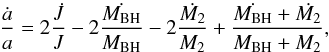 (4)where a single dot defines the first-order derivative with respect to time.
In the analytic point-mass MT model, exchange and loss of angular momentum occurs as a result of exchange of mass between the two point masses, or by the removal of mass from one of the two point masses. When mass is transferred to or lost from the vicinity of a point mass, it carries the specific orbital angular momentum j = rω2 of that point mass. We only considered RLO through the Lagrangian point L1, which in general is the dominating MT mechanism in LMXBs and IMXBs (Tauris 2006). During RLO, a fraction α of the mass lost from the donor (Ṁ2) will escape the system on its way to the accretor, carrying the specific orbital angular momentum of the donor; that is, angular momentum exchange in the accretion flow is ignored. The remaining fraction 1-α is funnelled through the L1 point toward the accretor. A fraction β of the mass transferred through the L1 point, that is, β(1−α)Ṁ2, will be lost from the system from the vicinity of the accretor, carrying its specific angular momentum. The remaining fraction (1−β)(1−α)Ṁ2 will be accreted onto the accretor. The mass change of the BH is ṀBH = −(1−α)(1−β)Ṁ2 and the time derivative of the angular momentum is given as 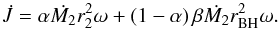 (5)As we only consider transfer of mass, we can ignore the time-dependent mass change rate Ṁ2 and instead use the transformation
  to obtain the orbital evolution as a function of M2. The orbital evolution given by Eq. (4)of the system during RLO MT ignoring other potential angular momentum loss mechanisms then becomes
 ![\begin{equation} \frac{{\rm d}a}{{\rm d}M_{2}} = \frac{2a}{M_{2}}\left[\alpha(1-q)-(1-q)+\frac{q}{2(1+q)}(\alpha \beta- \alpha - \beta)\right]. \label{eq:dadM2} \end{equation}](/articles/aa/full_html/2017/01/aa28979-16/aa28979-16-eq85.png) (6)We solve this equation analytically to derive the orbital period P as a function of the donor mass M2 and use Eq. (2)to obtain
(6)We solve this equation analytically to derive the orbital period P as a function of the donor mass M2 and use Eq. (2)to obtain  (7)where MBH = MBH,RLO + (1−β)(1−α)(M2,RLO−M2) and the subscript RLO refers to initial system values at the onset of RLO. Equation (7)is only valid for β ≠ 1, M2,RLO ≠ 0 and MBH,RLO ≠ 0. For β = 1 Eq. (6)is reduced, and a new analytic solution can be found. For the case where β = 1 the time dependent mass change rate of the accreting BH vanishes and the solution to Eq. (6)then is
  (8)For each combination of initial parameters PRLO, M2,RLO, MBH,RLO, α and β, we find the root of the equation P(M2) = Pobs, where Pobs is the currently observed orbital period of LMC X-3. The root of this equation, if it exists, gives us the mass M2,cur that the donor has when the orbit reaches the observed period. From this, we can also calculate the current mass of the BH as MBH,cur = MBH,RLO + (1−β)(1−α)(M2,RLO−M2,cur). From the current mass of the BH and the donor star we obtain the mass ratio q. If the calculated q and MBH,cur are farther away than two standard deviations from the observed current values (see Table 1), then this combination of PRLO, M2,RLO, MBH,RLO, α, and β values is excluded from a further search of the parameter space because a binary with these properties at the onset of RLO is not a PPS of LMC X-3.
As the BH is accreting mass from the donor, not only the BH mass changes, but also its angular momentum. We assumed here that the material being accreted by the BH carries the specific angular momentum of the BH’s innermost stable circular orbit (ISCO). For a BH with initial mass Mi and zero spin at the onset of RLO and total mass-energy ℳ once some material has been accreted, where  , the dimensionless Kerr spin parameter is
 ![\begin{equation} \label{eq:BH_spin} a_{\ast} = \left(\frac{2}{3}\right)^{\tfrac{1}{2}}\frac{M_{\rm i}}{\mathcal{M}}\left[4-\sqrt{\frac{18M_{i}^2}{\mathcal{M}^2}-2}\right], \end{equation}](/articles/aa/full_html/2017/01/aa28979-16/aa28979-16-eq102.png) (9)for 0 ≤ a∗ ≤ 1 (Thorne 1974).
(9)for 0 ≤ a∗ ≤ 1 (Thorne 1974).
The relation between the accreted rest mass M0−M0i since RLO onset, the BH initial total mass-energy Mi, and the total mass-energy ℳ is ![\begin{equation} \label{eq:Maccret} M_0 - M_{0i} = 3M_{\rm i}\left[\sin^{-1}\left(\frac{\mathcal{M}}{3M_{\rm i}}\right)-\sin^{-1}\left(\frac{1}{3}\right)\right]\cdot \end{equation}](/articles/aa/full_html/2017/01/aa28979-16/aa28979-16-eq105.png) (10)Here M0i = 0 assuming the BH has not accreted any mass before RLO onset and the total accreted rest mass is M0. We also assumed that a∗ = 0 at RLO onset, meaning that the natal spin of the BH is negligible, which was shown to be a reasonable assumption to explain the Galactic BH LMXB population (Fragos & McClintock 2015). Under these assumptions, solving Eq. (10)with respect to ℳ and inserting it into Eq. (9)yields the BH spin parameter for an accreted amount of rest mass M0. Finally, for the sake of completeness, we also include the case
(10)Here M0i = 0 assuming the BH has not accreted any mass before RLO onset and the total accreted rest mass is M0. We also assumed that a∗ = 0 at RLO onset, meaning that the natal spin of the BH is negligible, which was shown to be a reasonable assumption to explain the Galactic BH LMXB population (Fragos & McClintock 2015). Under these assumptions, solving Eq. (10)with respect to ℳ and inserting it into Eq. (9)yields the BH spin parameter for an accreted amount of rest mass M0. Finally, for the sake of completeness, we also include the case  and a∗ = 1 where
 ![\begin{equation} \mathcal{M} = 3^{- \tfrac{1}{2}}M_0-3^{\tfrac{1}{2}}M_{\rm i} \left[\sin^{-1}\left(\frac{2}{3}\right)^{\tfrac{1}{2}} - \sin^{-1}\left(\frac{1}{3}\right)\right] + 6^{\tfrac{1}{2}}M_{\rm i}. \end{equation}](/articles/aa/full_html/2017/01/aa28979-16/aa28979-16-eq111.png) (11)The solution of Eq. (9)is shown in Fig. 1 for different initial BH masses at RLO onset. Here the evolution of the BH spin parameter is tracked as a function of accreted mass.
(11)The solution of Eq. (9)is shown in Fig. 1 for different initial BH masses at RLO onset. Here the evolution of the BH spin parameter is tracked as a function of accreted mass.
 |
Fig. 1 Evolution of the BH spin parameter, given by Eq. (9), for a set of BH initial masses Mi as a function of accreted mass M0 Eq. (10). The gray areas mark the 1σ and 2σ errors centered on the observed spin parameter for LMC X-3 (see Table 1). The vertical dashed black lines indicate the maximum allowed accreted mass M0, at 2σ limit for an initial non-spinning BH mass of 5 M⊙ (left) and 8 M⊙ (right), respectively. |
For reference, centered on the LMC X-3 spin parameter a∗ = 0.25, we added the 1σ and 2σ error region as the dark and light gray areas, respectively. A low initial BH mass requires less accreted mass, in absolute terms, to build up its spin parameter compared to higher initial BH masses. As an example, we can follow a BH with initial mass Mi = 5.0 M⊙ (blue line) as it accretes mass and compare it to a BH with initial mass Mi = 8.0 M⊙ (black line). The blue line reaches the upper spin parameter after accreting ~1 M⊙ and reaches a current mass of 6 M⊙. The black line reaches the upper spin parameter limit when it has accreted ~1.6 M⊙ and has a mass of 9.6 M⊙. In terms of relative mass accreted to initial BH mass, both BHs accrete ~20% of their initial BH mass before reaching the upper spin parameter limit of LMC X-3, so that their initial BH mass was ~83.3% of the current mass when accretion began. Hence, the maximum amount of accreted material onto the BH of LMC X-3 is ~16.6% of its current mass. The LMC X-3 BH has a lower mass limit MBH = 5.86 M⊙ within 2σ. A lower limit of the BH mass at RLO onset therefore becomes (1−0.166)5.86 M⊙ ~ 4.9 M⊙.
When we instead consider the observed mass of the LMC X-3 BH and accept a 2σ limit, its current upper mass limit is 8.1 M⊙. This means that a BH of initial mass 8.0 M⊙ cannot have accreted more than 0.1 M⊙, suggesting that such a BH in the case of LMC X-3 should have a spin parameter a∗ ~ 0.04.
We stress that we used the observed BH spin of LMC X-3 only as a condition to constrain the upper limit of the amount of mass that the BH can possibly have accreted since the onset of the RLO. In reality, the BH in LMC X-3 may have been formed with a non-zero natal spin, in which case the limits on the maximum accreted mass discussed above would be upper bounds.
 |
Fig. 2 Solid, dashed, and dotted lines represent examples of a binary system undergoing RLO and MT for different sets of initial values at the onset of RLO. The vertical dashed line is the observed orbital period given in Table 1. The color map indicates the relative likelihood log (ℒi/ ℒmax) from Eq. (14). The thickening of the color bands around the observed orbital period denotes that in this region all model parameters ℐi,j, different from the one being plotted, are within 2σ of the observed value from Table 1. In all panels but f) and h), the dark and light gray regions are centered on the observed value, and each gray contrast extends to an area of ±1σ and ±2σ, respectively. The black lines in panel d) are the critical MT rate, Eq. (13). The light gray lines in panel h) are the Eddington accretion rate (Frank et al. 2002). We note that all three examples displays first a case A MT where core-hydrogen burning takes place. The sudden changes seen at periods equal to 3.1, 3.4, and 3.7 days are the transition from case A MT to case B MT, where the donor star has formed a helium core and hydrogen-shell burning has commenced. Computation of the three examples shown are stopped before case B MT is completed, when the orbital period reaches six days. |
In summary, we note that the analytic point-mass MT model together with the BH spin parameter is a powerful yet computational inexpensive tool to establish rough but meaningful bounds on our four-dimensional parameter space in determining whether a set of initial conditions at RLO onset leads to a MT sequence that satisfies the observational constraints on Pobs, MBH, and M2. To account for the remaining observational constraints, X-ray luminosity, Teff, R2, log g2, and donor luminosity L2, we need to model the stellar evolution of the companion star in detail.
3.2. Detailed MESA calculation
Our detailed simulations of the MT phase between the donor star and the BH were computed with MESA, a publicly available 1D stellar structure and binary evolution code. We adopted a metallicity for the donor star appropriate for LMC stars (Z = 0.006; which is in line with derived metallicities of stellar populations in LMC, Antoniou & Zezas 2016) and used the implicit MT scheme incorporated in MESA. All our simulations were calculated with revision 7184 of the code1. We explored the initial parameter space at the onset of RLO by constructing a grid of MT sequences for M2,RLO in the range 2–15 M⊙ in steps of 0.2 M⊙, orbital periods PRLO from 0.6–4.2 days in steps 0.1 day, and MBH,RLO from 5.0–8.0 M⊙ in steps of 0.5 M⊙. We also varied the accretion efficiency parameter β, considering values of β = 0.0, 0.25, 0.5, 0.75, 0.9, and 1.0. In all our calculations we set the accretion efficiency parameter α = 0.0, as a non-zero value would be appropriate only for massive donor stars that lose a significant amount of mass in the form of fast stellar winds (van den Heuvel 1994). To speed up the computation of individual models, we invoked a stopping criterion within MESA that terminates the computation once the orbital period is longer than six days. Of all possible combinations of M2,RLO, MBH,RLO, PRLO and β, we only ran detailed MESA calculations for those sets of initial conditions that passed our analytic MT model test, which we described in Sect. 3.1.
To identify those MT sequences that are PPS of LMC X-3 at the moment of RLO onset, we performed the following checks:
-
1.
The ZAMS radius of the donor star is smaller than itsRoche-lobe radius at the onset of RLO.
-
2.
When RLO begins, the donor star is younger than the Universe (<13.7 Gyr). Furthermore, the MT calculations are terminated when the age of the donor reaches 13.7 Gyr, so that the system today cannot be older than the age of the Universe either. In practice, neither of these constraints limits our calculations here because of the range of donor star masses that we explored.
-
3.
During the MT phase, as the orbital period is evolving, it should cross the observed period Pobs.
-
4.
A MT sequence model ℐ has j = [1,5] predicted parameters that all must be within 2σ of the observed quantities μj given their associated errors σj, which are both listed in Table 1,
 (12)where ℐi,j are the predictions of the ith MT sequence for each of these quantities at the time when the orbital period of the MT sequence is equal to the observed period.
 -
5.
Infer whether the predicted accretion rate onto the BH by the specific MT system would cause it to appear as a transient or a persistent X-ray source.
The latter check separates the MT sequences into two regimes of MT mechanisms. When the MT rate into the accretion disk is Ṁ2<Ṁcrit, where 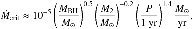 (13)the system is in a transient state, otherwise the system is in a persistent state (Dubus et al. 1999). A persistent source has a continuous flow of material from the donor star to the BH, which allows for a relatively high luminosity. If the source is transient, it goes through periods of outbursts of high X-ray flux but spends most of its time with little to no X-ray flux, or in other words, in a quiescent phase.
Under the assumption of constant MT efficiency, that is, constant α and β, MT sequences passing checks 1 through 4 are PPS that predict a system with characteristics similar to currently observed properties of LMC X-3. In principle α and β are average values for the efficiency of the MT and therefore merely serve as an indicator of whether a semi-conservative or non-conservative transfer of mass is needed.
Assuming that the reported errors for all observed quantities in Table 1 are Gaussian, then the likelihood of a model MT sequence, ℐi, given the currently observed data, D, of LMC X-3 can be written as 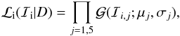 (14)where
  is a normalized Gaussian function, and μj and σj for j = [1,5] are the observed values and the associated errors listed in Table 1. In principle, the likelihood of a MT sequence, when the sequence is crossing the observed period, is an estimate of how close the specific model MT sequence comes to the observed properties of LMC X-3. We intend to use Eq. (14)as a weight to produce a series of probability density functions (PDF) in Sect. 4.2. In this case, we also multiply the likelihood value calculated by Eq. (14)by the time period, ΔT, that a model MT sequence spent close to the observed orbital period. This time period is defined as the total time during which all parameters j are within 2σ of the observed properties.
3.3. Constraining the properties of LMC X-3 progenitor at the onset of the Roche-lobe overflow
With the checks defined in the previous section, we now present three examples of individual MT sequences and compare them to the observational parameters in Table 1. The examples are chosen to demonstrate how the constraints select some MT sequences as PPS and discard others.
All three examples are plotted together in Fig. 2 and have initial parameters at the onset of RLO: β = 0.75, MBH,RLO = 6.5 M⊙, M2,RLO = 7.8 M⊙, and PRLO = 1.0 days (dotted lines); β = 0.90, MBH,RLO = 6.0 M⊙, M2,RLO = 7.4 M⊙, and PRLO = 0.8 days (dashed lines); β = 0.90, MBH,RLO = 6.0 M⊙, M2,RLO = 8.0 M⊙, and PRLO = 0.8 days (solid lines). Along the x-axis of all panels the orbital period P is shown in days and the vertical dashed line marks the currently observed orbital period Porb (see Table 1). The color bar shows the relative likelihood ℒi/ ℒmax, as determined from Eq. (14)for all parameters j. For all three examples, a maximum likelihood is reached as the MT sequence model crosses the observed orbital period. In each panel a through h, a thickening of the color indicates that all parameters ℐi,j apart from the one being plotted, as indicated on each y-axis, are within 2σ of the observed value. The gray areas shown in some of the panels indicate the 1σ and 2σ (dark and light gray, respectively) error regions of those parameters centered on the observed values, similar to Fig. 1.
Panel a of Fig. 2 shows the evolution of the donor star’s effective temperature with orbital period. The solid and dashed lines are within 2σ of Teff,obs as they cross the observed orbital period and are thickened, indicating that all other model parameters j are also within the 2σ region of their observed values. The solid and dashed lines are likewise thickened in all panels in Fig. 2, close to the observed orbital period. The dotted line is thickened in panels a and b, but falls outside the effective temperature 2σ region and therefore is not thickened in the other panels of Fig. 2, indicating that the specific MT sequence does not represent a PPS. Qualitatively, the effective temperature decreases until the orbital period reaches 3.1, 3.4, and 3.7 days, where it briefly spikes, signaling the end of the donor’s MS. Following the spike, the effective temperature continues its decrease, although it has experienced a slight increase relative to that before the spike.
Panel b of Fig. 2 shows the donor mass, M2, as a function of the orbital period. The donor mass M2 does not experience any changes around orbital periods of 3.1, 3.4, and 3.7 days, indicating that the changes observed in temperature are due to the donor star internal structure and not the result of sudden changes in the secular evolution of the binary system. We recall that the donor mass is not used to derive the relative likelihoods, nor is it included as a constraining parameter; instead, the mass ratio q is.
The donor radius R2, shown in panel c, increases as the orbital period increases. As the star evolves away from the MS, the donor star radius increases to the Roche lobe limit, causing a mass loss. With this mass loss, the orbit expands, the Roche-lobe radius increases, and the donor star radius can increase further. This process continues until the donor star reaches the end of H burning, where the donor star radius shows a contraction at orbital periods of 3.1, 3.4, and 3.7 days. Following the contraction, the donor star expands to fill its Roche lobe again. During the MS the donor radius increases because its core molecular weight increases, which results in a denser and more luminous core, causing the above layers to expand (Maeder 2008). With the decrease in mass and increase in radius of the donor star, its surface gravity also decreases (not shown), similar to the effective temperature.
In contrast to the monotonically decreasing mass of the donor star, the evolution of the mass-loss rate  , shown in panel d of Fig. 2, varies widely. It begins with a rapid turn-on phase, when the donor star fills its Roche lobe, and then gradually declines as the mass-ratio of the binary decreases. The initial turn-on phase rapidly reaches a peak MT rate near 10-6M⊙ yr-1 and then drops by nearly an order of magnitude, where it stabilizes to a steady slow decrease until an orbital period of 3.1 days for the solid line, 3.4 days for the dashed, and 3.7 days for the dotted lines. At this point, the rate drops below 10-10M⊙ yr-1 and the binary temporarily detaches, but MT commences again with a rate of ~10-5.5M⊙ yr-1, which is roughly sustained until the whole envelope of the donor star is removed (see also Sect. 5.6 where the evolution of LMC X-3 after its currently observed state is described). During the entire MT phase the models predict a persistent source. The mass-loss rate of the donor star M2 qualitatively dictates the accretion rate onto the BH shown in panel h of Fig. 2, but is higher by a factor (1−β)-1.
 |
Fig. 3 Grid of MT sequences for different MT efficiencies of α = 0.0 and β = [0.0, 0.25, 0.5, 0.75, 0.90, and 1.0], from the left to the right columns of the panels. Each row, as labeled at the right of the figure, corresponds to an initial value of MBH,RLO = [5.0, 5.5, 6.0, 6.5, 7.0, 7.5, and 8.0] M⊙. On the x-axis of each panel are shown the initial mass of the donor star M2,RLO, the range of which is allowed to vary with β. The y-axis shows the initial orbital period PRLO in days. Gray areas correspond to regions with initial MBH,RLO, M2,RLO, and PRLO values that do not pass the analytic MT test or the initial ZAMS radius is greater than the Roche lobe. The white areas represent initial combinations of MBH,RLO, M2,RLO, and PRLO that pass the analytic MT model, and for which we have made a detailed simulation with MESA. Circles indicate MT sequences that fail check 4, squares pass all checks and are persistent solutions according to Eq. (13). The colors indicate the relative likelihood of each detailed run. |
Panel e of Fig. 2 shows the change in the system mass ratio, which increases as material is transferred to the BH or is lost from the system. For the three examples shown, both their mass ratio and donor mass at the orbital period are within 2σ. However, there are combinations of donor mass and BH mass for which the mass ratio is outside the 2σ region.
In panel f of Fig. 2, we show the evolution of the BH mass as a function of orbital period. The accretion onto the BH is initially mildly super-Eddington, but declines rapidly. Especially for the dashed and solid lines with β = 0.9, the BH mass-accretion rate reaches a plateau with only a small gain in mass as the orbital period lengthens. For the solid line with β = 0.75 the BH mass increase is larger, while at the same time the orbit expands faster. All three lines satisfy the observed BH mass constraint at the crossing period. The BH spin a∗, shown in panel g, is a measure of the accreted angular momentum by the BH, as we assumed a zero natal BH spin. We find that the evolution of the BH spin follows the characteristics of the BH mass, that is, the growth in spin is steep initially and flattens as the orbital period increases.
Finally, panel h shows the BH mass-accretion rate as a function of orbital period. The light gray lines are the Eddington accretion rates (Frank et al. 2002) for each MT sequence. The changes in the BH mass-accretion rate with orbital period are similar to the mass-loss rate of the companion star, but scaled with the value close to β, which is the fraction of transferred mass that is lost from the system in the vicinity of the BH. The BH accretion rate is also affected by the sudden change in radius and effective temperature of the companion star, at orbital periods of 3.1, 3.4, and 3.7 days. Following the second MT turn-on event, the BHs in the three example sequences accrete close to the Eddington accretion rate and are potentially mildly super-Eddington.
The three examples shown in Fig. 2 all show the same qualitative evolution, but because of the differences in their initial conditions display the changes at different orbital periods. The radial contraction seen at the same time as the increase in effective temperature and surface acceleration, at 3.1, 3.4, and 3.7 days, indicates that the donor star is restructuring its interior. Its core has depleted its hydrogen, stopped nuclear burning, and left behind a helium core. As a result, the core luminosity briefly drops, whereby the envelope contracts, meaning that the donor radius decreases, and the effective temperature and surface acceleration increase. As a consequence of the contraction, a shell of hydrogen at the bottom of the envelope ignites, pushing the envelope beyond its pre-contraction radius. Hence the three examples in Fig. 2 are case A RLO MT until an orbital period of 3.1, 3.4, and 3.7 days, where the hydrogen-shell burning forces the envelope outward and the three examples enter a RLO MT of case B (Kippenhahn & Weigert 1967). In single star evolution, a star entering the hydrogen-shell burning increases its radius dramatically, by approximately two orders of magnitude (Tauris 2006), and the star enters the Red Giant Branch (RGB). The donor star is prevented from evolving to the RGB phase while undergoing RLO. While the expansion experienced by the donor star leads it to overfill its Roche Lobe on the one hand, its increased radius enhances the mass lost from its outer layers. The net effect is to contain the star at its Roche radius. Near shell-burning ignition the donor star has lost ~60% of its ZAMS mass. Owing to our stop criteria at an orbital period of 6 days, the three examples shown in Fig. 2 do not enter the helium-burning phase. The change rate in orbital period during case A MT is slow (not shown), and during the case B MT phase it increases dramatically, such that the entire evolution shown during case B MT in Fig. 2 only takes a few 105 yr. The donor star in our three examples has lost as much as ~70% of its ZAMS mass by the time our simulations stop. For our MT sequences we expect the donor star’s stellar evolution to end with the formation of a He white dwarf (WD), or in the cases of the most massive donors, a carbon-oxygen WD.
By reviewing the evolution of three selected MT sequence models, one that passes items 1–3 (dotted line), defined in Sect. 3.2, two that pass items 1–4, we are confident in our checks as a filter to locate PPS of LMC X-3 at the moment of RLO onset. As we also show, we can distinguish between transient and persistent systems. The calculated relative likelihood shows a maximum for all three examples close to the orbital period, which validates our approach. We next consider the overall result of our detailed MT sequences.
3.4. Results of modeling the X-ray binary phase
In Fig. 3 we show the initial conditions of our grid of 3319 MT sequences. Each column of the panels represents MT sequences for different values of β (top axis). Each row varies the initial value of MBH,RLO in units of M⊙ (right axis). On the x-axis within each panel we plot the companion mass M2,RLO in units of M⊙ and on the y-axis the orbital period PRLO in days. The gray areas indicate regions where any combination of initial values fails the analytic MT model. The white areas denote combinations of initial values that pass the analytic MT model. With increasing β, the relative size of the area that passes the analytic model increases as well. As a result, we allowed the horizontal size of each panel and x-axis range to change with β to better display the content of each figure.
Each circle and square represents a set of initial conditions of a binary system immediately before initiation of RLO that was simulated with MESA. Circles are those MT sequences that failed check 4, while squares are those sequences that passed all checks and are persistent solutions. The figure clearly shows that the number of PPS increases with β.
The color represents the relative likelihood of a particular MT sequence model to the model with maximum weight, similar to that used for Fig. 2, displaying individual MT sequences. We note that while in Fig. 2 we show the relative likelihood as a function of orbital period, in Fig. 3 we display the value of the relative likelihood of each MT sequence at the observed orbital period. The set of initial conditions with the highest likelihood is β = 1.0, MBH,RLO = 7.5 M⊙, M2,RLO = 8.2 M⊙, and PRLO = 0.8 days, which is a persistent solution. Of the 3319 MT sequences simulated with MESA, 395 are PPS of LMC X-3 at the moment of RLO onset.
Selected properties of 20 MT sequences that pass all criteria at the observed orbital period.
PPS property ranges at the RLO onset found from MT sequences with the analytic model and MESA.
Setup of our population synthesis models using BSE (first five columns).
In Table 2 selected properties of our solutions to the RLO MT sequence of LMC X-3 are shown2. Our grid of MT sequences is most successful in finding PPS when the RLO MT happens non-conservatively, with a donor star mass between M2,RLO = 4.20−9.80 M⊙, a MBH,RLO = 5.5−8.0 M⊙, and an orbital period PRLO = 0.8–1.7 days. In Table 3 we outline the range of initial values at the moment of RLO onset for the donor mass, BH mass, mass fraction of lost material from the accretor, and the current age of the system, as found from the analytic MT model and MESA. In addition to the actual ranges found, we have in post processing also included the ranges of winners from MESA were we impose an Eddington accretion limit for material accreted onto the BH. This causes changes in the mass of the BH and its spin. We have ignored the effect to the orbital evolution. Applying the Eddington mass accretion limit in general increases the number of winning sequences by 2, to 397 MT sequences. The most notable change is the range of the donor mass M2,RLO whose upper limit is reduced to 8.6 M⊙ from 9.80 M⊙. Finally, there is a slight change in the maximum estimated age of the system. For all values of β the mean difference in mass accreted between models with and without the Eddington accretion limit is 0.044 M⊙ and only for β = 0 the difference is noteworthy (0.21 M⊙). If one, on the other hand look at the maximum difference in mass accreted between the two sets of models, this ranges from 0.63 to 1.1 M⊙ for different values of β.
4. From the ZAMS to the RLO
Before becoming a BH XRB, LMC X-3 began its evolution as a newly formed binary system in a wide and potentially eccentric orbit. Given its high initial mass, the primary star quickly inflated as it evolved off the MS, eventually filling its Roche lobe and initiating MT onto the secondary. The high mass ratio of the primary to the secondary star meant that the MT occurred fast and was thermally and most likely dynamically unstable. In this dynamically unstable MT phase, also known as CE phase, the secondary star orbits within the tenuous envelope of the primary star, spirals inward because of friction, and heats the envelope. The CE phase results in either the merger of the two stars or in the ejection of the primary’s envelope, making the system a detached binary of a He core and a MS companion on a close and circular orbit.
Eventually, the He core that is left from the CE phase enters the core-collapse phase and becomes a BH. During the SN explosion, asymmetries may alter the orbit further and might even disrupt the system. When this is not the case, the binary system now comprises a BH and companion star, where tidal forces may change the orbit further. The companion star is largely unaffected during this process and continues its stellar evolution to eventually reach the onset of RLO. In this section, we investigate the range of PPS at the ZAMS stage that can lead to the appropriate characteristics at RLO onset.
4.1. Population synthesis study with the binary stellar evolution code
During the formation of the BH binary and before the onset of RLO, many physical processes as described above take place. These processes are difficult to model, computationally expensive, and are not yet fully understood from first principles. Even if all the physical processes could be modeled in detail, our estimate of the LMC X-3 progenitor properties at the onset of RLO can only provide a probable range and is influenced by uncertainties in the observationally constrained parameters given in Table 1. Therefore, when searching for PPS at the ZAMS, these uncertainties propagate backward and increase the range of PPS properties even more. A more approximate approach is therefoee sufficient for the purpose of estimating the pre-RLO onset characteristics of LMC X-3 PPS. Such an estimate can be achieved with the Binary Stellar Evolution code (BSE; Hurley et al. 2002), which is a fast parametric binary evolution code that allows simulating large sets of binary systems, accounting for all relevant physical processes such as stellar microphysics, CE, CO formation, and SN dynamics.
We have modified BSE to include the suite of stellar wind prescriptions for massive stars described in Belczynski et al. (2010), the fitting formulae for the binding energy of the envelopes of stars derived by Loveridge et al. (2011), and the prescriptions “STARTRACK”, “Delayed”, and “Rapid” for CO formation in binaries, as described in Fryer et al. (2012). Each CO formation prescription favors a different distribution of CO masses as a function of ZAMS mass and corresponds to different formulations of the engines driving supernovae based on their metallicity, initial ZAMS mass, and pre-SN core mass. See Fryer et al. (2012) for an elaborate description of the prescriptions.
As input to the population synthesis models we used the same set of 108 binary systems that was sampled as follows: The primary star M1,init was sampled from a Kroupa initial stellar mass function (Kroupa 2001, IMF) with α = 2.3 and M1,init = [20:40] M⊙, and we assumed in general that a Kroupa IMF can describe the distributions of stars of the LMC. We drew a binary mass ratio qinit = [0:0.5] from a uniform distribution, and combined with M1,init, this gave the secondary stellar mass M2,init. Third, the orbital separation was sampled from a logarithmically uniform distribution in the range ]0:5] (R⊙). The fourth parameter sampled is the eccentricity, which was drawn from the thermal eccentricity distribution (Jeans 1919). From these four parameters an initial orbital period was determined using Kepler’s third law (Eq. (2)).
A total of ten different models were simulated with BSE, varying the CO mass prescription, the CE efficiency αCE = 0.0, 0.5, 1.0, and 2.0 and the distribution of kick velocities that BHs may receive during the SN. For the latter we considered a Maxwellian distribution with σv = 26.5, 100.0, and 265.0 km s-1, a uniform distribution with an upper limit of 2000 km s-1, and the limiting case of no kicks. A Maxwellian distribution with 265.0 km s-1 is known to describe the natal kick distribution for single pulsars (Hobbs et al. 2005), and here we explore whether it might also be qualitatively relevant for natal kicks in BH formation. By using different values for αCE and σv we avoid favoring one particular setup against another, hence recognizing that knowledge on both the CE phase and the natal kick distribution remain uncertain. Model 1 was chosen as our reference model (see Table 4).
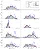 |
Fig. 4 Probability density function (PDF) of initial masses of the companion star M2,ZAMS for the different synthesis population models in Table 4. The gray bar is a normalized histogram, and the different colored lines are normalized kernel density estimates for different weights found from Eq. (14)and shown in the inset of this figure, for individual factors j and for the total weight given as the product over all j times the time spent around the orbital period, which is the black line. |
4.2. Results of the population synthesis study
Each synthetic binary system was simulated from initial values at ZAMS, again using the metallicity Z = 0.006, forward to the companion star RLO onset. Those systems that match a MESA MT sequence model were stored with relevant information of the system at the ZAMS, the moment immediately before the SN explosion, the moment immediately after the explosion, and at the onset of RLO. The kick velocity Vkick and peculiar post-SN velocity Vpec,postSN, following the explosion, were also recorded. We defined a match between the MESA MT sequence and a single BSE system when the system at the onset of RLO predicted by BSE was within 0.05 days of the orbital period, 0.1 M⊙ of the donor mass, and 0.25 M⊙ of the BH mass, of one of the MT sequences simulated with MESA. We only matched BSE solutions with the 395 MT sequences identified as LMC X-3 PPS from modeling the X-ray MT phase, see Sect. 3.4.
The second rightmost column of Table 4 shows the number of PPS for each population synthesis model. The reference model 1 generated 1322 PPS out of a total of 108 simulated binaries, suggesting at a first glance a relatively low formation rate, but see the discussion in Sect. 4.1. In models 2, 3, and 4 we varied the CE efficiency parameter, with αCE = 0.1, 0.5, and 2.0 for each model, respectively, and we found that the number of PPS increases with αCE. In models 5, 6, and 7 we varied the distribution of natal BH kicks, with the most probable kick velocity being σv = 0.0, 26.5, and 100 km s-1 for each model, respectively, also finding an increasing number of PPS with increasing σv. Model 8 adopts the STARTRACK prescription for the mass of CO formed, generating a small number of PPS, while in model 9 the Rapid prescription for CO formation was used, producing a number of PPS comparable to model 1.
The small number of PPS produced from models 2 and 8 are statistically insignificant samples of PPS to reliably estimate the range of LMC X-3 PPS at ZAMS. Based on the very low formation efficiency of these two models, we can only infer that it is possible, but highly unlikely, that LMC X-3 is formed from the settings of these models. For LMC X-3 this suggests that the CE phase is necessary, and that the STARTRACK prescription is a poor estimate of the CO mass. For model 4, which is the model that most efficiently forms PPS, it is hard to justify the high value of αCE, but it also indicates that the CE phase is important for generating LMC X-3 like systems. Since model 2 produced only 1 PPS, we did not include it in the remaining analysis.
Based on the number of PPS for each model, we performed a statistical analysis using weighted kernel density estimators (KDE). A Gaussian kernel was used to produce a probability density estimate for each relevant property of PPS during the evolution of the LMC X-3. In Fig. 4 we demonstrate how the PDF of the companion star mass at ZAMS, M2,ZMAS, will look for each population synthesis model for different weights. The weights were determined using a single factor in Eq. (14), that is, only ℐi,j and a weight based on the time a MT sequence spends around the currently observed properties of LMC X-3. The latter is defined as the time a MT sequence spends within two standard deviations of all the observed constraints. Finally, the total weight, which is the product, or the left-hand side, of Eq. (14)ℐi multiplied by the time spent around the observed orbital period. The gray bar plot is a normalized histogram, and the dashed line is a non-weighted KDE. The remaining lines are KDEs with different weights as described by the legend. It is shown that the unweighted KDE produces a continuous distribution that follows closely the discrete distribution of the histogram. The total weight Eq. (14)over all j, relative to the other distributions, concentrates the most likely solution into two peaks except for models 5, 6, and 8. The most likely values based on the total weight also show the two peaks to fall away from the peak of the unweighted distribution, the cause of which is the emerging distribution of using counts together with weights. The distribution using the total weight finds a different maximum because the weights near the maximum with no weights are much smaller, by several orders of magnitude, than the weights at the maximum of the distribution with the total weight (see the color scale of Fig. 3, which displays the values of the total weights). In the remaining analysis we use the total weight in all our distributions.
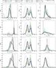 |
Fig. 5 PDF of the properties of LMC X-3 progenitors (M1, M2, and a) at different evolutionary stages, at ZAMS, pre-SN, post-SN, and onset of RLO, for the different synthesis population models in Table 4. The PDFs are weighted with the total weight. |
Figure 5 shows the overall most likely evolution of LMC X-3, from its initial binary properties at ZAMS (top panel), to pre-SN (second row), post-SN (third row), and finally at RLO onset (bottom row) for the different population synthesis models, expressed as PDFs. The PDFs are produced as KDEs with the total weight applied, as defined earlier. Each color is a model from Table 4 (see the figure legend). We have de-emphasized four models by presenting them in gray, three of these (models 5, 6, and 8) because they have small or insufficient numbers of PPS to be statistical representable. Model 4 is also grayed out, but instead owing to its unphysical setting of αce = 2. The latter model was considered mostly to examine the sensitivity of the number of PPS to this parameter.
The remaining models 1, 3, 7, 9, and 10 have model parameters that are physically plausible and produce a sufficiently large number of PPS. These models estimate the values, at different evolutionary stages, of the properties of the LMC X-3 progenitor to be in the same range, along the x-axis of each panel. The peak of each distribution also seems to be at the same x-values, but for places with a bimodal distribution, the individual model favors the peaks differently.
The initial value of M1,ZAMS at the 95% percentile is in the range 25.4–31.0 M⊙ when considering all models except model 4. Model 4 has a range 22.4–30.1 M⊙. All models suggest that the primary mass immediately before the SN is close to M1,preSN ~ 17.8M⊙, although models 4, 7, and 10 also suggest a minor peak around ~12 M⊙. After the SN, the range of the CO masses is M1,postSN = 6.4–8.2 M⊙ (95%).
The secondary star M2 experiences less dramatic changes than the primary M1; it evolves from a ZAMS to a BH. This is expected as M2 during this time is still on the MS, and during the first MT episode the secondary mass star does not gain significant mass. There are two most probable values for the donor mass, one around 6.8 M⊙ favored by models 1, 3, 4, and 9. The second peak is around 8 M⊙ and is favored by models 7 and 10. The mass range spanned by all models is 5.0–8.4 M⊙ (95%).
The orbital separation is initially very large, but as the primary star evolves away from the MS, it fills its Roche lobe, and the binary enters a CE phase, resulting in a significantly closer binary orbit. At the moment immediately before the SN, a has decreased by a factor of ~300 from several thousand solar radii to ~10 R⊙. The orbital separation following the SN favors a value of ~9 R⊙.
The distribution of the most likely kicks imparted during the BH formation is shown in Fig. 6 and the post-SN peculiar velocity is shown in Fig. 7, which is due to both the kick imparted and the mass lost. Models 1, 3, 4, and 9 suggest the same distribution for the imparted kick and follow from the fact that these four models had the same input distribution. The range of these four models is roughly between Vkick = 196–683 km s-1 (95%), with only models 5, 6, and 7 suggesting kicks less than 120 km s-1, which is expected given the lower most probable kick value for these models. Thus, the actual lower limit of Vkick may likely be closer to 120 km s-1. Notably, model 7, which uses σv = 100 km s-1, still shows a peak kick at ~180 km s-1, which supports the demand for an appreciable kick in the BH formation. Model 10 applied an uniform kick distribution and finds PPS within the range Vkick = 212–912 km s-1 (95%). All in all, the distribution of Vkick in the different population synthesis models indicates that a relatively high kick velocity is likely to be imparted to the LMC X-3 progenitor system. We find in our simulations that some models produce PPS with smaller or no kicks, but the associated probability is low relative to models favoring high kicks. The consequence of the kick, assuming it does not disrupt the system, is a perturbation of the system’s center of mass motion or the post-SN peculiar velocity. In addition to the kick, material lost from the system through the primary also affects the post-SN peculiar velocity Vpec,postSN (Kalogera 1996; Willems et al. 2005,see Fig. 7), as this mass is ejected off-center of the binary system center of mass. Overall, the Vpec,postSN in Fig. 7 is comparable in magnitude to the kick velocity shown in Fig. 6. For all models except model 7, more than 90% of the PPS have Vkick>Vpec,postSN. In models 6 and 7 only ~11% and ~27% have a larger kick velocity than Vpec,postSN, and for model 5 the Vpec,postSN is always larger than the relating Vkick. For model 10 with a uniform kick distribution ~99% have Vkick>Vpec,postSN.
4.3. Example of full evolution from the ZAMS to white dwarf formation
In Fig. 8 we illustrate the complete evolution of a typical LMC X-3 PPS from the ZAMS until the companion star becomes a WD. The system chosen is the MESA MT sequence with a relative high likelihood for the X-ray binary phase and one of its BSE matches for the evolution before the X-ray phase, hence representative of our results. The evolution begins with a primary star of mass M1,ZAMS = 26.5M⊙ and its companion star with mass M2 = 8 M⊙ in a wide and highly eccentric orbit. The primary star evolves quickly and fills its Roche lobe, leading to a CE phase that shrinks and circularizes the orbit. During the CE phase, the donor star spirals inward within the primary envelope. Because of friction, the envelope is heated and expelled, leaving behind a detached binary of a naked He core and the donor star. The remaining He core of the primary eventually experiences a SN explosion at ~8 Myr and collapses into a BH. During the SN, the BH receives a natal kick Vkick = 497 km s-1. 4.2 Myr later at time =12.2 Myr, the companion star fills its Roche lobe, and mass starts flowing from the donor star onto the BH. The system is now an observable X-ray source until a time of 58.8 Myr, where the MT briefly stops for a few Myr. At ~62 Myr MT is initiated again for a short period of time (~0.5 Myr). The brief pause is the end of the donor’s MS evolution. During this pause, the donor star contracts and restructures its interior, and the system develops from a case A MT into a case B MT. Following the pause, the donor star is in a shell H-burning phase with a He core. Because the orbit and thus the companion star radius expands during the shell burning, and also because of the intense MT, the donor Teff drops to a minimum value. Eventually, when the envelope of the companion star is almost completely removed, the companion star contracts well within its Roche lobe and the binary detaches. At this point, the MT stops and the effective temperature of the companion star increases fast, indicating that what is left is a degenerate low-mass helium core on its way to becoming a helium WD. The final binary consists of a 12.1 M⊙ BH with spin a∗ = 0.63, and a 0.6 M⊙ He WD on a 96-day orbit.
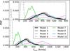 |
Fig. 6 PDF of the kick imparted to LMC X-3 during the SN for the different synthesis population studies. The inset gives a more detailed view of the distribution in the x-axis range from 0 to 800 km s-1 and follows the same axis labels, and the plotted lines have the same legend. |
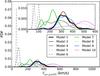 |
Fig. 7 PDF of LMC X-3’s center of mass velocity or LMC X-3’s peculiar post SN velocity, for the different population synthesis models. The insert gives a more detailed view of the distribution in the x-axis range from 0 to 600 km s-1 and follows the same axis labels and the plotted lines have the same legend. |
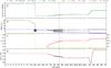 |
Fig. 8 Illustration of the complete evolution of a typical LMC X-3 PPS from the ZAMS to a double CO (BH+WD) binary. Panel a) shows the evolution of the orbital period in days on a logarithmic scale. Panel b) displays the evolution of the masses in the binary system; the primary star M1 as a star and as a BH (black line), and the companion star M2 (blue line). The black star label indicates the time of BH formation. Panel c) shows the evolution of the system eccentricity e in yellow, while in red we show the BH spin parameter a∗. Panel d) shows the effective temperature Teff of the donor star on a logarithmic scale. Data from the BSE simulation are shown as dashed lines, while data from MESA as plotted solid lines. From Table 1 we have added in panel a) the observed orbital period as the green dotted line, in panel b) the 1σ and 2σ error of M2 and MBH centered on the observed values, in panel c) the red dotted line is the upper 2σ limit on the BH spin parameter, and in panel d) the 1σ and 2σ error of Teff. In general, there is a fine agreement between BSE and MESA at the moment of RLO, except for the age of the system at RLO onset. MESA calculations find that RLO onset occurs at time =8.8 Myr, whereas BSE finds it to begin at time =12.2 Myr. The reason for the discrepancy is the differences in the micro physics, between BSE and MESA, and in particular in the stellar structure calculations. Here, for illustrating purposes, the MESA calculations are offset to the right by 2.4 Myr to generate a smooth transition in the figure. The star marks the formation of the BH at ~8 Myr and the vertical dashed line marks the time ~42 Myr at which the system crosses the observed orbital period. |
View of the most likely range based on weighted 25–75 (5–95) percentiles for each BSE model, one model per column.
4.4. Expected number of IMXB within the LMC today
In our reference model (model 1 in Table 4), which is most efficient in producing LMC X-3 PPS (excluding the unphysical models), we found 1322 PPS out of 108 model binary systems. We found fewer PPS for the model with the delayed CO formation prescription (model 9), and even fewer with the STARTRACK prescription (model 8) or small natal kicks. Here we address the question of the number of IMXBs that are predicted to be observable today within the LMC, for a given population synthesis model, regardless of whether their binary properties resemble those of LMC X-3.
To do so, we defined an IMXB as any binary system with a BH and a companion star of mass 3 ≤ M2/M⊙< 10 that experiences RLO MT. To estimate the number of IMXBs produced in the LMC within some period of time T, we made a population synthesis model for a new sample of binary systems. The new sample follows the same distributions as described in Sect. 4.1, but with the range of the Kroupa IMF set to M1,ZAMS = [10,100]M⊙ and qinit = ] 0,1 ]. This ensures that the new sample is sufficiently broad to not only produce a subset of binary systems relevant for a subset of IMXB, but can produce all IMXB within our definition. In the end, we corrected our identified number of IMXB NBSE,IMXB with the expected fraction of stars within the sample range fIMF [10;100]. Making the sample sufficiently large also ensures that a statistical significant number of IMXBs is produced. The sample size is NBSE,sim = 2 × 10⁷ binary systems. The number of IMXB produced within the LMC during the time period T is then given as ![\begin{equation} N_{\rm IMXB, LMC}(T) = \frac{N_{\rm BSE,IMXB}}{N_{\rm BSE,sim}}f_{\rm IMF}[10;100]N_{\rm bin}(T), \end{equation}](/articles/aa/full_html/2017/01/aa28979-16/aa28979-16-eq270.png) (15)where Nbin(T) is the number of binary systems produced in the LMC within a time period T. From our definition of IMXB, the population synthesis model yields a maximum IMXB age to be ~300 Myr, hence we set T = 300 Myr. Nbin is then estimated by assuming a mean star formation rate in the LMC over the past 300 Myr of ~0.2 M⊙ yr-1 (Harris & Zaritsky 2009) and a mean stellar mass of 0.518 M⊙ based on a binary fraction of 70%, a Kroupa IMF, and a uniform mass ratio distribution within binary systems. We obtain Nbin = 0.7 × 0.5 × 0.2 M⊙ yr-1 × 300 Myr / 0.518 M⊙ = 4 × 10⁷. The IMF correction fIMF [10;100] = 0.0014 was found by integrating the normalized IMF in the mass range [10;100] M⊙. The number of produced IMXB within LMC in the past 300 Myr is then NIMXB,LMC = 4.45 systems.
(15)where Nbin(T) is the number of binary systems produced in the LMC within a time period T. From our definition of IMXB, the population synthesis model yields a maximum IMXB age to be ~300 Myr, hence we set T = 300 Myr. Nbin is then estimated by assuming a mean star formation rate in the LMC over the past 300 Myr of ~0.2 M⊙ yr-1 (Harris & Zaritsky 2009) and a mean stellar mass of 0.518 M⊙ based on a binary fraction of 70%, a Kroupa IMF, and a uniform mass ratio distribution within binary systems. We obtain Nbin = 0.7 × 0.5 × 0.2 M⊙ yr-1 × 300 Myr / 0.518 M⊙ = 4 × 10⁷. The IMF correction fIMF [10;100] = 0.0014 was found by integrating the normalized IMF in the mass range [10;100] M⊙. The number of produced IMXB within LMC in the past 300 Myr is then NIMXB,LMC = 4.45 systems.
To derive the expected number of observable IMXBs today within the LMC, NIMXB,LMC,Obs, we multiplied by the mean life time of IMXBs,  , that is, the time that they are X-ray bright as IMBXs, over the relevant period T:
  (16)From the BSE simulation used to estimate the number of IMXBs formed, we also derived the mean lifetime of IMXBs to be
  Myr for model 1. Hence, the expected number of observable IMXBs within the LMC for model 1 is 0.72 system. This is consistent with the fact that we only observe one IMXB system in the LMC today, which is LMC X-3. Column 7 of Table 4 yields the result for all BSE models.
5. Discussion
5.1. Initial separation and eccentricity distribution
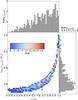 |
Fig. 9 Distribution of log (aZAMS) vs. eZAMS with the total weight applied for all identified LMC X-3 PPS. The top panel shows the weighted histogram of eZAMS and the bottom right histogram shows the distribution of log (aZAMS). The 2D-histogram with the total weight applied has the eccentricity at ZAMS along the x-axis and the orbital separation at ZAMS along the y-axis. The color bar shows the PDF of the 2D-histogram. |
Figure 9 shows a 2D-histogram of the (eZAMS,aZAMS) plane of LMC X-3 PPS at ZAMS compiled by all ten BSE models into one. The histogram is weighted with the total weight and normalized. Although aZAMS was sampled in the logarithmic range ]0;5], an initial separation >103.2R⊙ is needed to form a LMC X-3 PPS, but eZAMS spans the entire range from nearly circular to highly eccentric orbital shapes. The 2D-histogram reveals that for log (aZAMS/ days) < 3.5eZAMS< 0.78 and for log (aZAMS/R, ⊙) > 3.5eZAMS> 0.52. Additionally, as the top panel in Fig. 9 we added the PDF of all eZAMS with the total weight applied. It shows that eccentric orbits are more probable than nearly circular orbits. To the right in Fig. 9 we show the PDF of aZAMS. The orbital separation is found to be 3.2 < log (aZAMS/R, ⊙) < 4. Overall, increasing the initial orbital separation also increases the eccentricity. Hence very wide orbits are highly eccentric. Had the wide systems been circular, they would not fill their Roche lobe the first time to begin the CE phase. In consequence, these systems would not develop into XRB.
5.2. Natal spin of the BH
In the analytic MT model introduced in Sect. 3.1, we made the explicit assumption that the natal spin of the BH is zero. This is motivated from the recent work by Fragos & McClintock (2015). The authors suggested that BH progenitor stars of Galactic BH LMXBs loose most of their angular momentum before the onset of the CE as a result of wind mass-loss and envelope expansion during the giant phase, and they showed that the currently observed BH spin in Galactic LMXBs can be explained as solely due to accretion after the BH formation. However, no direct observational or theoretical evidence that the natal spin of BHs in Galactic LMXBs is negligible is available so far.
In the context of our analysis, the assumption of zero natal spin is in fact a conservative one. This is because we only required the mass that the BH accretes from the onset of the RLO phase until its current state does not spin up the BH to a value of a∗ that is higher than two sigma above the observed value. If a non-zero natal BH spin is assumed, then the maximum amount that the BH in LMC X-3 may have accreted after its formation is further constrained to a lower value. This has as a direct effect that the lowest allowed natal mass of the BH increases, but it should in principle also narrow down the allowed range of all the binary properties of the system at the onset of RLO. Table 6 shows how these ranges change for a choice of natal BH spin of a∗ ,natal = 0.1 and a∗ ,natal = 0.2, relative to our standard assumption of zero natal spin. However, because it remains an open question how exactly BH form and how the formation process may affect their natal spin, we decided to adopt the most conservative wider range of allowed RLO properties, which corresponds to a natal BH spin of a∗ ,natal = 0. As Table 6 shows, although individual MT sequences may not qualify anymore as PPS, there are almost no changes in the overall estimated ranges. Only the minimum present age of the system increases as the natal spin increases, and it is barely noticeable for a∗ = 0.1. The minimum age increases because the more massive donors on a small orbit will begin their RLO early enough to spin up the BH above the allowed spin limit. Assuming no natal spin, we find a total of 395 MT sequences as PPS for LMC X-3, and for a natal spin of 0.1 and 0.2 we find 371 and 336 PPS, respectively. As a limiting case, we may consider the BH spin to be entirely natal, hence accretion onto the BH would not be possible. This would be equivalent to our case of MT sequences with β = 1.
5.3. X-ray flux of LMC X-3
In Fig. 10 we compare the accretion rates onto the BH as inferred from the successful MESA MT sequence models from Sect. 3.4 to the observed values from Steiner et al. (2014a). The black solid line is the distribution of the observed instantaneous accretion rates, while the red lines correspond to the long-term average accretion rate estimates from persistent MESA MT sequences. The black dashed vertical line is the critical MT rate for the development of the disk thermal instability, given from Eq. (13), using the observed values of LMC X-3 from Table 1.
Overall, the observed accretion rates cover a wider range, whereas the MT sequence models distribute themselves with most likely accretion rates near the critical accretion rate given by Eq. (13)for the observed properties of LMC X-3 from Table 1. We should stress here that a direct comparison between the observations and the model predictions is not possible. This is because the observed instantaneous accretion rates cover a baseline of ~10 yr, while our modeled MT sequences yield an average value over timescales of a few 105 to several 106 yr and do not include any potential short-term fluctuations. Keeping this in mind, the general agreement between our predictions and the data at hand is notable and suggests an affirmation of our model. The fact that our MT calculations predict MT rates close to the transition region between transient and persistent sources provides a natural explanation for the atypical X-ray variability of LMC X-3.
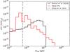 |
Fig. 10 Distribution of observationally determined instantaneous accretion rates onto the BH taken at different times (black), and distribution of long-term average BH accretion rates inferred from MT sequence, calculated with MESA, that successfully reproduce the observed characteristics of LMC X-3 (red). The vertical black dashed line shows the critical MT rate for the thermal disk instability model, given by Eq. (13), for the observationally inferred properties given in Table 1. |
5.4. Mechanism of compact object formation
Although we see quantitative differences between the three different CO prescriptions, Rapid, Delayed, and STARTRACK as a SN mechanism to have produced LMC X-3, we cannot make a global ruling between the three prescriptions on this basis. It is evident, however, that STARTRACK cannot reproduce a statistically significant set of PPS for LMC X-3. The Rapid and Delayed prescriptions both produce comparable results. We examined how the three prescriptions perform in producing a population of IMXB, as we did in Sect. 4.4. The result of repeating the population synthesis study (Sect. 4.4) for IMXB in the LMC using the STARTRACK prescription yields that 0.98 IMXB is currently observable within the LMC. The Delayed prescription yields a total of 0.73 systems is currently observable. In conclusion, all three prescriptions give a consistent number of IMXB in the LMC relative to observations. The same can be said for the other individual models in Table 4 with varying αCE and σv.
5.5. Natal kicks and the orbit of LMC X-3 within the LMC
An interesting aspect of our synthesis population study with BSE is the increase in the PPS number when we increase σv of the assumed Maxwellian asymmetric kick distribution from 0 km s-1 to 265 km s-1. Only few PPSs are found when no kick or only a small kick is imparted. By gradually increasing the kick to be imparted until it equals the NS kick distribution, we increase the number of PPSs. Most noticeable is the jump from σv = 26.5 km s-1 to σv = 100 km s-1, where the number of PPSs increases by a factor ~10. Although we do not have direct evidence, the indication is strong that LMC X-3 has probably formed with a kick being imparted to it. Given the lack of sufficiently precise peculiar motion measurements of LMC X-3, which would allow us to set direct constraints on the natal kick that the BH received, our estimates depend on the model assumed for the compact object formation. The reason is that the latter dictates the relation between the pre-SN mass of the BH progenitor and its natal BH mass, and hence the amount of mass lost during SN. A high mass-loss during SN tends to result in wide post-SN orbits, for which in turn a large kick in the appropriate direction is required to maintain tight orbits.
The estimated post-SN peculiar velocity or systemic velocity of the binary center-of-mass is also relatively high. Even for cases with zero or small kicks, the systemic velocity is most likely higher than 50 km s-1. This is due to the high mass-loss from the primary during the SN (see Fig. 5). This relative high post-SN system velocity requires a kinematic study of the LMC X-3 within the LMC. Given the high systemic velocity that the system may have received, it should affect the system orbit within the parent galaxy. The current shape of this orbit might be extrapolated from sufficiently accurate measurements of the system’s three-dimensional motion and the known potential of the LMC, from which it might be tested whether LMC X-3 is on a normal orbit, which would most likely suggest a low kick and low systemic velocity. If instead LMC X-3 were found to have a peculiar orbit, it would suggest that the system would have received a high kick and high systemic velocity. Finally, if the LMC X-3 were in an extreme orbit or would perhaps even have escaped the LMC, it would indicate that the LMC X-3 received a very high kick. In this respect it might be possible to constrain the imparted lower or upper natal kick.
For LMC X-3 only the radial velocity is measured with accuracy. Observations of radial velocities, which are somewhat survey dependent, suggest a radial velocity of Vrad = 300–308 km s-1; see Table 1 in Orosz et al. (2014). Using the model of van der Marel et al. (2002) updated with the numbers of van der Marel & Kallivayalil (2014), we can derive the expected radial velocity of a system in the LMC. This model gives an expected radial velocity of 244 km s-1 for LMC X-3, which compared to actual observations yields a difference of ~55km s-1. This in turn suggests that the LMC X-3 center-of-mass rest frame is moving faster than its neighboring stellar population even when accounting for a velocity dispersion of ~20 km s-1 (van der Marel & Kallivayalil 2014). The proper motion of LMC X-3 is μαcos(δ) = −2.7 mas yr-1 ± 24.4 and μδ = 12.5 ± 24.4 mas/yr-1 (Smart & Nicastro 2014), which if translated into a 3D velocity, yields uncertainties so high that it cannot be used to constrain the past evolution of LMC X-3.
5.6. LMC X-3: The young sibling of GRS 1915+105?
A comparison of our MT sequences from MESA to the Galactic LMXB GRS1915+105, which has the fastest measured spin of all LMXBs a∗> 0.98 (McClintock et al. 2006), provides some interesting insights. Overall GRS1915+105’s current properties are P = 33.85 days (Steeghs et al. 2013), MBH = 12.4 ± 2.0 M⊙ (Reid et al. 2014), M2 = 0.52 ± 0.41 M⊙ (McClintock 2016, priv. comm.), donor spectral type K0III-K3II and Teff = 4766.5 ± 666.5 K (Harlaftis & Greiner 2004; Greiner et al. 2001; Gray 2008; Cox 2000).
For our comparison we reran the best-fit LMC X-3 MT sequences with β = 0, allowing as much mass transferred as possible, and compared them to the parameters of GRS 1915+105 at its current orbital period. For the masses MBH, M2, and Teff we accepted models that are within 2σ at the observed orbital period. For the BH spin parameter we made no constraint. We found 11 MT sequence models that match the GRS1915+105 parameters and have a BH spin in the range 0.76 to 0.86. Figure 11 shows the comparison of one MT sequence model (see legend for settings at RLO onset). In the three panels we show the Teff, M2, and MBH as a function of orbital period. The color bar shows the BH spin parameter while the BH is accreting material. When the color thickens, the properties of the MT sequence model are within 2σ of the currently observed properties of GRS 1915+105. The evolution of the system is initially similar to that described in Sect. 3.3. The abrupt increase in Teff at the end of the evolution is the formation of a WD. The similarity between the evolution of LMC X-3 based on our simulations and of GRS1915+105 indicate that these two systems may have formed from similar progenitor binary systems. Finally, although the best-fit MT sequences for LMC X-3 with β = 0 can reach BH spins a∗> 0.8, it is clear that the combination of donor and BH masses at the onset of RLO does not provide a sufficiently high mass reservoir to spin up the BH to an extreme spin. As shown in Fragos & McClintock (2015), the range of donor masses at RLO onset that are required to spin up the BH in GRS 1915+105 to a∗> 0.98 is slightly higher than our inferred range for LMC X-3. Relaxing our assumption for negligible natal spin for GRS 1915+105 would yield a much larger overlap between the PPSs for the two systems. On the other hand, this would indicate a different compact object formation process for the BHs in the two systems.
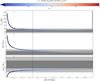 |
Fig. 11 Best-fit MT sequence simulated with MESA from RLO onset (see legend for values) and onward until the donor becomes a WD. In the three panels, the observed properties of the Galactic LMXB GRS 1915+105 are shown, indicated by the gray areas. The light and dark gray areas are centered on the observed values of GRS 1915+105, and each gray contrast spans 1σ on each side, except for M2, where the lower 2σ limit is truncated at 0. The dashed vertical line is the observed orbital period of 33.85 days of GRS1915+105. The color shows the BH spin parameter a∗ which for GRS 1915+105 is a∗> 0.98, and it shows the fastest spin to be below 0.9. The thickening of the color denoting the MT sequence in each panel indicates the part of the evolutionary track for which the model properties are within 2σ of the observed properties of GRS 1915+105 (excluding the BH spin). The sudden spike seen in the top panel is the formation of a WD. |
6. Conclusion
In a two-part study, we have reconstructed the evolution of LMC X-3 from its current X-ray bright MT phase back to when the system was at the ZAMS. In the first part we formulated an analytic MT point-mass model for the XRB phase that includes binary component mass and orbital angular momentum changes, as well as changes in the spin parameter of the BH. The analytic MT point-mass model was used to initially limit the possible parameter space of the LMC X-3 PPS at the moment of RLO onset, for which we then performed detailed numerical simulations with MESA. We computed a regular space grid of 3319 MT sequences, of which 395 are solutions of the RLO onset settings of LMC X-3, all of which are persistent sources. From our detailed MT sequences we found that the current MT rate of LMC X-3 is close to the critical MT rate predicted by the thermal instability disk model, which defines the boundary between a persistent and transient source. This might explain the high X-ray variability of LMC X-3 along with the fact that the system has always been bright since its discovery.
We then used the range of solutions at RLO onset found from MESA to match a large set of binary population synthesis simulations performed with BSE. We considered ten different models with BSE, and for each model we estimated the most likely range for PPSs of LMC X-3 at the ZAMS, immediately before the SN, immediately after the SN, and at the onset of RLO. In addition, we recorded the natal kick imparted to the BH during the SN and the systemic velocity after the kick. Overall, we find at 95 % confidence across all models that LMC X-3 began as a ZAMS binary with a primary of mass M1,ZAMS = 22.4–31.0 M⊙, a secondary at M2,ZAMS = 5.0–8.3 M⊙, an orbital period of PZAMS = 2000−400 000 days, and an eccentricity eZAMS ≥ 0.18. Immediately before the SN, the primary had a mass M1,preSN = 11.1−18.0 M⊙, with the secondary star largely unaffected, although it might have accreted some of the mass lost from the primary. From ZAMS to immediately before the SN, the orbit decreased to periods between 0.6–1.7 days, and epreSN ≤ 0.44. We found systems without a natal kick, but these are few, and it is much more likely that the SN explosion imparted a large kick of 120 km s-1 or more. Following the SN, the system has a BH of M1,postSN = 6.4–8.2 M⊙ on an eccentric orbit. From the time immediately after the SN and until the RLO onset, the orbit is circularized and has a period of PRLO = 0.8–1.4 days.
Finally, we discussed whether the evolution of LMC X-3 might have been similar to the much older Galactic LMXB GRS1915+105. We demonstrated that LMC X-3 will likely not build up an equally extreme spin because the LMC X-3 system overall has too little mass to accumulate such an extreme spin through accretion. Despite this, it is likely that GRS1915+105 was also an IMXB when its RLO began, and followed a similar evolution starting with a slightly higher mass companion star.
In summary, we have successfully traced the evolution of LMC X-3 from a ZAMS binary system until its current state. Studying LMC X-3 and constraining its characteristics, especially during the CO formation, is of great importance for the understanding of how BH IMXB form and evolve. From an observational point of view, we also offer a likely explanation for the high X-ray variability associated with LMC X-3 by estimating the current long-term average MT rate close to the boundary between transient vs. persistent behavior. Our prediction that the system likely received a large natal kick and has a correspondingly large post SN peculiar velocity might be tested with sufficient kinematic data and a proper motion study.
The detailed MESA settings used in out simulations can be found at http://mesastar.org/results
Acknowledgments
This work was supported by the Swiss National Science Foundation (project number 200020-160119). We thank the anonymous referee for constructive suggestions that improved this manuscript. M.S. is grateful for support from the Swiss National Science Foundation and to the StarPlan Center, University of Copenhagen where much of this work was performed. T.S. acknowledges support from the Ambizione Fellowship of the Swiss National Science Foundation (grant PZ00P2_148123). J.F.S. has been supported by NASA Einstein Fellowship grant PF5-160144. The computations were performed at the University of Geneva on the Baobab cluster. All figures were made with the free Python module Matplotlib (Hunter 2007).
References
- Antoniou, V., & Zezas, A. 2016, MNRAS, 459, 528 [NASA ADS] [CrossRef] [Google Scholar]
- Antoniou, V., Zezas, A., Hatzidimitriou, D., & Kalogera, V. 2010, ApJ, 716, L140 [NASA ADS] [CrossRef] [Google Scholar]
- Belczynski, K., & Bulik, T. 2002, ApJ, 574, L147 [NASA ADS] [CrossRef] [Google Scholar]
- Belczynski, K., Bulik, T., Fryer, C. L., et al. 2010, ApJ, 714, 1217 [NASA ADS] [CrossRef] [Google Scholar]
- Belczynski, K., Bulik, T., & Bailyn, C. 2011, ApJ, 742, L2 [NASA ADS] [CrossRef] [Google Scholar]
- Bondi, H. 1952, MNRAS, 112, 195 [NASA ADS] [CrossRef] [MathSciNet] [Google Scholar]
- Brocksopp, C., Groot, P., & Wilms, J. 2001, MNRAS, 328, 139 [NASA ADS] [CrossRef] [Google Scholar]
- Brown, G. E., Lee, C.-H., & Moreno Méndez, E. 2008, ApJ, 685, 1063 [NASA ADS] [CrossRef] [Google Scholar]
- Cowley, A. P. 1992, ARA&A, 30, 287 [NASA ADS] [CrossRef] [Google Scholar]
- Cowley, A., Crampton, D., Hutchings, J., Remillard, R., & Penfold, J. 1983, ApJ, 272, 118 [NASA ADS] [CrossRef] [Google Scholar]
- Cowley, A., Schmidtke, P., Ebisawa, K., et al. 1991, ApJ, 381, 526 [NASA ADS] [CrossRef] [Google Scholar]
- Cox, A. N. 2000, in Allen’s astrophysical quantities (AIP Press, Springer) [Google Scholar]
- Cui, W., Feng, Y. X., Zhang, S. N., et al. 2002, ApJ, 576, 357 [NASA ADS] [CrossRef] [Google Scholar]
- Dosopoulou, F., & Kalogera, V. 2016a, ApJ, 825, 70 [NASA ADS] [CrossRef] [Google Scholar]
- Dosopoulou, F., & Kalogera, V. 2016b, ApJ, 825, 71 [NASA ADS] [CrossRef] [Google Scholar]
- Dubus, G., Lasota, J.-P., Hameury, J.-M., & Charles, P. 1999, MNRAS, 303, 139 [NASA ADS] [CrossRef] [Google Scholar]
- Fragos, T., & McClintock, J. E. 2015, ApJ, 800, 17 [NASA ADS] [CrossRef] [Google Scholar]
- Fragos, T., Kalogera, V., Willems, B., et al. 2009, ApJ, 702, L143 [NASA ADS] [CrossRef] [Google Scholar]
- Fragos, T., Tremmel, M., Rantsiou, E., & Belczynski, K. 2010, ApJ, 719, L79 [NASA ADS] [CrossRef] [Google Scholar]
- Fragos, T., Linden, T., Kalogera, V., & Sklias, P. 2015, ApJ, 802, L5 [NASA ADS] [CrossRef] [Google Scholar]
- Frank, J., King, A., & Raine, D. 2002, Accretion power in astrophysics (Cambridge University Press) [Google Scholar]
- Fryer, C. L., Belczynski, K., Wiktorowicz, G., et al. 2012, ApJ, 749, 91 [NASA ADS] [CrossRef] [Google Scholar]
- Gou, L., McClintock, J. E., Reid, M. J., et al. 2011, ApJ, 742, 85 [NASA ADS] [CrossRef] [Google Scholar]
- Gray, D. F. 2008, in The Observation and Analysis of Stellar Photospheres (Cambridge, UK: Cambridge University Press) [Google Scholar]
- Greiner, J., Cuby, J. G., McCaughrean, M. J., Castro-Tirado, A. J., & Mennickent, R. E. 2001, A&A, 373, L37 [NASA ADS] [CrossRef] [EDP Sciences] [Google Scholar]
- Harlaftis, E. T., & Greiner, J. 2004, A&A, 414, L13 [NASA ADS] [CrossRef] [EDP Sciences] [Google Scholar]
- Harris, J., & Zaritsky, D. 2009, AJ, 138, 1243 [NASA ADS] [CrossRef] [Google Scholar]
- Hobbs, G., Lorimer, D. R., Lyne, A. G., & Kramer, M. 2005, MNRAS, 360, 974 [NASA ADS] [CrossRef] [Google Scholar]
- Hunter, J. D. 2007, Computing In Science & Engineering, 9, 90 [Google Scholar]
- Hurley, J. R., Pols, O. R., & Tout, C. A. 2000, MNRAS, 315, 543 [NASA ADS] [CrossRef] [Google Scholar]
- Hurley, J. R., Tout, C. A., & Pols, O. R. 2002, MNRAS, 329, 897 [NASA ADS] [CrossRef] [Google Scholar]
- Ivanova, N. 2006, ApJ, 653, L137 [NASA ADS] [CrossRef] [Google Scholar]
- Jeans, J. 1919, MNRAS, 79, 408 [NASA ADS] [CrossRef] [Google Scholar]
- Justham, S., Rappaport, S., & Podsiadlowski, P. 2006, MNRAS, 366, 1415 [NASA ADS] [CrossRef] [Google Scholar]
- Kalogera, V. 1996, ApJ, 471, 352 [NASA ADS] [CrossRef] [Google Scholar]
- Kippenhahn, R., & Weigert, A. 1967, Z. Astrophys., 65, 251 [NASA ADS] [Google Scholar]
- Kroupa, P. 2001, MNRAS, 322, 231 [NASA ADS] [CrossRef] [Google Scholar]
- Lee, C. H., Brown, G. E., & Wijers, R. A. M. J. 2002, ApJ, 575, 996 [NASA ADS] [CrossRef] [Google Scholar]
- Leong, C., Kellogg, E., Gursky, H., Tananbaum, H., & Giacconi, R. 1971, ApJ, 170, L67 [NASA ADS] [CrossRef] [Google Scholar]
- Li, X.-D. 2015, New Astron. Rev., 64, 1 [NASA ADS] [CrossRef] [Google Scholar]
- Linden, T., Sepinsky, J. F., Kalogera, V., & Belczynski, K. 2009, ApJ, 699, 1573 [NASA ADS] [CrossRef] [Google Scholar]
- Loveridge, A. J., Van der Sluys, M., & Kalogera, V. 2011, ApJ, 743, 49 [NASA ADS] [CrossRef] [Google Scholar]
- Maeder, A. 2008, in Physics, formation and evolution of rotating stars (Springer Science & Business Media) [Google Scholar]
- Mandel, I. 2016, MNRAS, 456, 578 [NASA ADS] [CrossRef] [Google Scholar]
- Mazeh, T., Van Paradijs, J., Van den Heuvel, E., & Savonije, G. 1986, A&A, 157, 113 [NASA ADS] [Google Scholar]
- McClintock, J. E., Shafee, R., Narayan, R., et al. 2006, ApJ, 652, 518 [NASA ADS] [CrossRef] [Google Scholar]
- McClintock, J. E., Narayan, R., & Steiner, J. F. 2013, Space Sci. Rev., 1, 73 [Google Scholar]
- Miller-Jones, J. C. A., Jonker, P. G., Dhawan, V., et al. 2009a, ApJ, 706, L230 [NASA ADS] [CrossRef] [Google Scholar]
- Miller-Jones, J. C. A., Jonker, P. G., Nelemans, G., et al. 2009b, MNRAS, 394, 1440 [NASA ADS] [CrossRef] [Google Scholar]
- Mirabel, I., Dhawan, V., Mignani, R. P., Rodrigues, I., & Guglielmetti, F. 2001, Nature, 413, 139 [NASA ADS] [CrossRef] [PubMed] [Google Scholar]
- Mirabel, I., Mignani, R., Rodrigues, I., et al. 2002, A&A, 395, 595 [NASA ADS] [CrossRef] [EDP Sciences] [Google Scholar]
- Moreno Méndez, E. 2011, MNRAS, 413, 183 [NASA ADS] [CrossRef] [Google Scholar]
- Moreno Méndez, E., Brown, G. E., Lee, C.-H., & Park, I. H. 2008, ApJ, 689, L9 [NASA ADS] [CrossRef] [Google Scholar]
- Moreno Méndez, E., Brown, G. E., Lee, C.-H., & Walter, F. M. 2011, ApJ, 727, 29 [NASA ADS] [CrossRef] [Google Scholar]
- Motta, S. E., Muñoz-Darias, T., Sanna, A., et al. 2014, MNRAS, 439, L65 [NASA ADS] [CrossRef] [Google Scholar]
- Naoz, S., Fragos, T., Geller, A., Stephan, A. P., & Rasio, F. A. 2016, ApJ, 822, L24 [NASA ADS] [CrossRef] [Google Scholar]
- Nugis, T., & Lamers, H. J. G. L. M. 2000, A&A, 360, 227 [NASA ADS] [Google Scholar]
- Orosz, J. A., Steiner, J. F., McClintock, J. E., et al. 2014, ApJ, 794, 154 [NASA ADS] [CrossRef] [Google Scholar]
- Paxton, B., Bildsten, L., Dotter, A., et al. 2011, ApJS, 192, 3 [Google Scholar]
- Paxton, B., Cantiello, M., Arras, P., et al. 2013, ApJS, 208, 4 [NASA ADS] [CrossRef] [Google Scholar]
- Paxton, B., Marchant, P., Schwab, J., et al. 2015, ApJS, 220, 15 [Google Scholar]
- Pietrzyński, G., Graczyk, D., Gieren, W., et al. 2013, Nature, 495, 76 [NASA ADS] [CrossRef] [PubMed] [Google Scholar]
- Piran, T., & Shaviv, N. J. 2005, Phys. Rev. Lett., 94, 051102 [NASA ADS] [CrossRef] [Google Scholar]
- Podsiadlowski, P., Rappaport, S., & Pfahl, E. D. 2002, ApJ, 565, 1107 [NASA ADS] [CrossRef] [Google Scholar]
- Podsiadlowski, P., Rappaport, S., & Han, Z. 2003, MNRAS, 341, 385 [NASA ADS] [CrossRef] [Google Scholar]
- Podsiadlowski, P., Langer, N., Poelarends, A. J. T., et al. 2004, ApJ, 612, 1044 [NASA ADS] [CrossRef] [Google Scholar]
- Podsiadlowski, P., Dewi, J. D. M., Lesaffre, P., et al. 2005, MNRAS, 361, 1243 [NASA ADS] [CrossRef] [Google Scholar]
- Rapley, C., & Tuohy, I. 1974, ApJ, 191, L113 [NASA ADS] [CrossRef] [Google Scholar]
- Reid, M., McClintock, J., Steiner, J., et al. 2014, ApJ, 796, 2 [NASA ADS] [CrossRef] [Google Scholar]
- Remillard, R. A., & McClintock, J. E. 2006, ARA&A, 44, 49 [NASA ADS] [CrossRef] [Google Scholar]
- Repetto, S., & Nelemans, G. 2015, MNRAS, 453, 3341 [NASA ADS] [CrossRef] [Google Scholar]
- Repetto, S., Davies, M. B., & Sigurdsson, S. 2012, MNRAS, 425, 2799 [NASA ADS] [CrossRef] [Google Scholar]
- Reynolds, C. S. 2013, Space Sci. Rev., 183, 81 [Google Scholar]
- Smart, R. L., & Nicastro, L. 2014, A&A, 570, A87 [NASA ADS] [CrossRef] [EDP Sciences] [Google Scholar]
- Soria, R., Wu, K., Page, M., & Sakelliou, I. 2001, A&A, 365, L273 [NASA ADS] [CrossRef] [EDP Sciences] [Google Scholar]
- Steeghs, D., McClintock, J. E., Parsons, S. G., et al. 2013, ApJ, 768, 185 [NASA ADS] [CrossRef] [Google Scholar]
- Steiner, J. F., McClintock, J. E., Orosz, J. A., et al. 2014a, ApJ, 783, 101 [NASA ADS] [CrossRef] [Google Scholar]
- Steiner, J. F., McClintock, J. E., Orosz, J. A., et al. 2014b, ApJ, 793, L29 [NASA ADS] [CrossRef] [Google Scholar]
- Tauris, T. M., & van den Heuvel, E. 2006, Compact stellar X-ray sources, 1, 623 [NASA ADS] [CrossRef] [Google Scholar]
- Thorne, K. S. 1974, ApJ, 191, 507 [Google Scholar]
- Valsecchi, F., Glebbeek, E., Farr, W. M., et al. 2010, Nature, 468, 77 [NASA ADS] [CrossRef] [Google Scholar]
- van den Heuvel, E. P. J. 1994, Saas-Fee Advanced Course of the Swiss Society for Astrophysics and Astronomy: Interacting binaries, 1, 263 [Google Scholar]
- Van der Klis, M., Tjemkes, S., & Van Paradijs, J. 1983, A&A, 126, 265 [NASA ADS] [Google Scholar]
- van der Marel, R. P., & Kallivayalil, N. 2014, ApJ, 781, 121 [NASA ADS] [CrossRef] [Google Scholar]
- van der Marel, R. P., Alves, D. R., Hardy, E., & Suntzeff, N. B. 2002, AJ, 124, 2639 [NASA ADS] [CrossRef] [Google Scholar]
- van Loon, J. T., Cioni, M. R. L., Zijlstra, A. A., & Loup, C. 2005, A&A, 438, 273 [NASA ADS] [CrossRef] [EDP Sciences] [Google Scholar]
- Warren, P., & Penfold, J. 1975, MNRAS, 172, 41P [NASA ADS] [CrossRef] [Google Scholar]
- Willems, B., Henninger, M., Levin, T., et al. 2005, ApJ, 625, 324 [NASA ADS] [CrossRef] [Google Scholar]
- Willems, B., Kaplan, J., Fragos, T., Kalogera, V., & Belczynski, K. 2006, Phys. Rev. D, 74, 043003 [NASA ADS] [CrossRef] [Google Scholar]
- Wong, T.-W., Valsecchi, F., Fragos, T., & Kalogera, V. 2012, ApJ, 747, 111 [NASA ADS] [CrossRef] [Google Scholar]
- Wong, T.-W., Valsecchi, F., Ansari, A., et al. 2014, ApJ, 790, 119 [NASA ADS] [CrossRef] [Google Scholar]
All Tables
Selected properties of 20 MT sequences that pass all criteria at the observed orbital period.
PPS property ranges at the RLO onset found from MT sequences with the analytic model and MESA.
View of the most likely range based on weighted 25–75 (5–95) percentiles for each BSE model, one model per column.
All Figures
|
Fig. 1 Evolution of the BH spin parameter, given by Eq. (9), for a set of BH initial masses Mi as a function of accreted mass M0 Eq. (10). The gray areas mark the 1σ and 2σ errors centered on the observed spin parameter for LMC X-3 (see Table 1). The vertical dashed black lines indicate the maximum allowed accreted mass M0, at 2σ limit for an initial non-spinning BH mass of 5 M⊙ (left) and 8 M⊙ (right), respectively. |
| In the text | |
|
Fig. 2 Solid, dashed, and dotted lines represent examples of a binary system undergoing RLO and MT for different sets of initial values at the onset of RLO. The vertical dashed line is the observed orbital period given in Table 1. The color map indicates the relative likelihood log (ℒi/ ℒmax) from Eq. (14). The thickening of the color bands around the observed orbital period denotes that in this region all model parameters ℐi,j, different from the one being plotted, are within 2σ of the observed value from Table 1. In all panels but f) and h), the dark and light gray regions are centered on the observed value, and each gray contrast extends to an area of ±1σ and ±2σ, respectively. The black lines in panel d) are the critical MT rate, Eq. (13). The light gray lines in panel h) are the Eddington accretion rate (Frank et al. 2002). We note that all three examples displays first a case A MT where core-hydrogen burning takes place. The sudden changes seen at periods equal to 3.1, 3.4, and 3.7 days are the transition from case A MT to case B MT, where the donor star has formed a helium core and hydrogen-shell burning has commenced. Computation of the three examples shown are stopped before case B MT is completed, when the orbital period reaches six days. |
| In the text | |
|
Fig. 3 Grid of MT sequences for different MT efficiencies of α = 0.0 and β = [0.0, 0.25, 0.5, 0.75, 0.90, and 1.0], from the left to the right columns of the panels. Each row, as labeled at the right of the figure, corresponds to an initial value of MBH,RLO = [5.0, 5.5, 6.0, 6.5, 7.0, 7.5, and 8.0] M⊙. On the x-axis of each panel are shown the initial mass of the donor star M2,RLO, the range of which is allowed to vary with β. The y-axis shows the initial orbital period PRLO in days. Gray areas correspond to regions with initial MBH,RLO, M2,RLO, and PRLO values that do not pass the analytic MT test or the initial ZAMS radius is greater than the Roche lobe. The white areas represent initial combinations of MBH,RLO, M2,RLO, and PRLO that pass the analytic MT model, and for which we have made a detailed simulation with MESA. Circles indicate MT sequences that fail check 4, squares pass all checks and are persistent solutions according to Eq. (13). The colors indicate the relative likelihood of each detailed run. |
| In the text | |
|
Fig. 4 Probability density function (PDF) of initial masses of the companion star M2,ZAMS for the different synthesis population models in Table 4. The gray bar is a normalized histogram, and the different colored lines are normalized kernel density estimates for different weights found from Eq. (14)and shown in the inset of this figure, for individual factors j and for the total weight given as the product over all j times the time spent around the orbital period, which is the black line. |
| In the text | |
|
Fig. 5 PDF of the properties of LMC X-3 progenitors (M1, M2, and a) at different evolutionary stages, at ZAMS, pre-SN, post-SN, and onset of RLO, for the different synthesis population models in Table 4. The PDFs are weighted with the total weight. |
| In the text | |
|
Fig. 6 PDF of the kick imparted to LMC X-3 during the SN for the different synthesis population studies. The inset gives a more detailed view of the distribution in the x-axis range from 0 to 800 km s-1 and follows the same axis labels, and the plotted lines have the same legend. |
| In the text | |
|
Fig. 7 PDF of LMC X-3’s center of mass velocity or LMC X-3’s peculiar post SN velocity, for the different population synthesis models. The insert gives a more detailed view of the distribution in the x-axis range from 0 to 600 km s-1 and follows the same axis labels and the plotted lines have the same legend. |
| In the text | |
|
Fig. 8 Illustration of the complete evolution of a typical LMC X-3 PPS from the ZAMS to a double CO (BH+WD) binary. Panel a) shows the evolution of the orbital period in days on a logarithmic scale. Panel b) displays the evolution of the masses in the binary system; the primary star M1 as a star and as a BH (black line), and the companion star M2 (blue line). The black star label indicates the time of BH formation. Panel c) shows the evolution of the system eccentricity e in yellow, while in red we show the BH spin parameter a∗. Panel d) shows the effective temperature Teff of the donor star on a logarithmic scale. Data from the BSE simulation are shown as dashed lines, while data from MESA as plotted solid lines. From Table 1 we have added in panel a) the observed orbital period as the green dotted line, in panel b) the 1σ and 2σ error of M2 and MBH centered on the observed values, in panel c) the red dotted line is the upper 2σ limit on the BH spin parameter, and in panel d) the 1σ and 2σ error of Teff. In general, there is a fine agreement between BSE and MESA at the moment of RLO, except for the age of the system at RLO onset. MESA calculations find that RLO onset occurs at time =8.8 Myr, whereas BSE finds it to begin at time =12.2 Myr. The reason for the discrepancy is the differences in the micro physics, between BSE and MESA, and in particular in the stellar structure calculations. Here, for illustrating purposes, the MESA calculations are offset to the right by 2.4 Myr to generate a smooth transition in the figure. The star marks the formation of the BH at ~8 Myr and the vertical dashed line marks the time ~42 Myr at which the system crosses the observed orbital period. |
| In the text | |
|
Fig. 9 Distribution of log (aZAMS) vs. eZAMS with the total weight applied for all identified LMC X-3 PPS. The top panel shows the weighted histogram of eZAMS and the bottom right histogram shows the distribution of log (aZAMS). The 2D-histogram with the total weight applied has the eccentricity at ZAMS along the x-axis and the orbital separation at ZAMS along the y-axis. The color bar shows the PDF of the 2D-histogram. |
| In the text | |
|
Fig. 10 Distribution of observationally determined instantaneous accretion rates onto the BH taken at different times (black), and distribution of long-term average BH accretion rates inferred from MT sequence, calculated with MESA, that successfully reproduce the observed characteristics of LMC X-3 (red). The vertical black dashed line shows the critical MT rate for the thermal disk instability model, given by Eq. (13), for the observationally inferred properties given in Table 1. |
| In the text | |
|
Fig. 11 Best-fit MT sequence simulated with MESA from RLO onset (see legend for values) and onward until the donor becomes a WD. In the three panels, the observed properties of the Galactic LMXB GRS 1915+105 are shown, indicated by the gray areas. The light and dark gray areas are centered on the observed values of GRS 1915+105, and each gray contrast spans 1σ on each side, except for M2, where the lower 2σ limit is truncated at 0. The dashed vertical line is the observed orbital period of 33.85 days of GRS1915+105. The color shows the BH spin parameter a∗ which for GRS 1915+105 is a∗> 0.98, and it shows the fastest spin to be below 0.9. The thickening of the color denoting the MT sequence in each panel indicates the part of the evolutionary track for which the model properties are within 2σ of the observed properties of GRS 1915+105 (excluding the BH spin). The sudden spike seen in the top panel is the formation of a WD. |
| In the text | |
Current usage metrics show cumulative count of Article Views (full-text article views including HTML views, PDF and ePub downloads, according to the available data) and Abstracts Views on Vision4Press platform.
Data correspond to usage on the plateform after 2015. The current usage metrics is available 48-96 hours after online publication and is updated daily on week days.
Initial download of the metrics may take a while.