| Issue |
A&A
Volume 683, March 2024
|
|
|---|---|---|
| Article Number | A85 | |
| Number of page(s) | 16 | |
| Section | Stellar structure and evolution | |
| DOI | https://doi.org/10.1051/0004-6361/202346880 | |
| Published online | 08 March 2024 | |
The X-ray binaries in M83: Will any of them form gravitational wave sources for LIGO-VIRGO-KAGRA?
Nicolaus Copernicus Astronomical Center, Polish Academy of Sciences, Bartycka 18, 00-716 Warsaw, Poland
e-mail: ikotko@camk.edu.pl
Received:
12
May
2023
Accepted:
14
December
2023
There are 214 X-ray point sources (LX > 1035 erg s−1) identified as X-ray binaries (XRBs) in the nearby spiral galaxy M83. Since XRBs are powered by accretion onto a neutron star (NS) or a black hole (BH) from a companion or donor star, these systems are promising progenitors of merging double compact objects (DCOs): BH-BH, BH-NS, or NS-NS systems. The connection (i.e., XRBs evolving into DCOs) may provide some hints to the as-yet-unanswered question: what is the origin of the LIGO, Virgo, and KAGRA mergers? Available observations do not allow us to determine what the final fate of the XRBs observed in M83 will be. However, we can use an evolutionary model of isolated binaries to reproduce the population of XRBs in M83 by matching model XRB numbers, types, and luminosities to observations. Knowing the detailed properties of M83 model XRBs (donor and accretor masses, and their evolutionary ages and orbits), we follow their evolution to the deaths of donor stars to check whether any merging DCOs are formed. Although all merging DCOs in our isolated binary evolution model go through the XRB phase (defined as reaching X-ray luminosity from RLOF or wind accretion onto NSs or BHs above 1035 erg s−1), only very few XRBs evolve to form merging (in Hubble time) DCOs. For M83, with its solar-like metallicity stars and continuous star formation, we find that only ∼1 − 2% of model XRBs evolve into merging DCOs depending on the adopted evolutionary physics. This is caused by (i) the merger of the donor star with a compact object during the common envelope phase, (ii) a binary disruption at the supernova explosion of a donor star, (iii) the formation of a DCO on a wide orbit (merger time longer than Hubble time).
Key words: gravitation / gravitational waves / binaries: close / stars: luminosity function / mass function / X-rays: binaries
© The Authors 2024
 Open Access article, published by EDP Sciences, under the terms of the Creative Commons Attribution License (https://creativecommons.org/licenses/by/4.0), which permits unrestricted use, distribution, and reproduction in any medium, provided the original work is properly cited.
This article is published in open access under the Subscribe to Open model. Subscribe to A&A to support open access publication.
1. Introduction
At the end of the third observing run, the LIGO-Virgo-KAGRA (LVK) collaboration reported ∼90 detections of gravitational wave signals from coalescing double compact objects (DCOs; Abbott et al. 2023). Among them, the vast majority (∼83) are double black hole (BH-BH) mergers, five are classified as black hole-neutron star (BH-NS) mergers, and only two are the confirmed mergers of two neutron stars (NS-NS). There are several formation scenarios that explain the origin of the merging DCOs. The leading ones are: the dynamical interactions in dense stellar systems (e.g. Portegies Zwart & McMillan 2000; Mapelli 2016; Rodriguez et al. 2018), the evolution of isolated binaries (e.g. Lipunov et al. 1997; Belczynski et al. 2010; Olejak & Belczynski 2021), the evolution of isolated multiple star systems (e.g. Toonen et al. 2016; Vigna-Gómez et al. 2021; Stegmann et al. 2022), the chemically homogeneous evolution of the isolated binaries (e.g. Mandel & de Mink 2016), the mergers of the binaries in active galactic nuclei (Antonini & Perets 2012; Fragione et al. 2019; Tagawa et al. 2020), and primordial black holes (BHs; De Luca et al. 2020; Clesse & García-Bellido 2022). At present there is no conclusion on the relative contribution of each of these channels to the formation of the observed gravitational wave (GW) sources. The fourth observational run of LVK, which started in May 2023 and is scheduled to collect data for over a year, is expected to significantly increase the number of detections by over ∼200 events (Petrov et al. 2022). The characteristics of these events may help to constrain which of the DCO evolutionary models are the most plausible.
While the merger is the final moment of the DCO’s life, the X-ray binaries (XRBs) are considered to be the DCO’s possible progenitors. XRBs are close binary systems where the mass is transferred from the donor star and accreted onto the compact object (NS or BH) giving rise to X-ray emission. Certain aspects of the evolution of the binary systems that enter the XRB phase still remain unclear. To constrain uncertainties in the binary star physics leading to the formation of XRBs, many groups use evolutionary codes to synthesize XRB populations and compare them with existing observations (e.g. Belczynski et al. 2008; Toonen et al. 2014; Eldridge & Stanway 2016; Fragos et al. 2023). The most straightforward comparison is done via the X-ray luminosity function (XLF, the cumulative distribution of X-ray luminosity of all the sources in a given sample) of a given XRB population (in one or more galaxies). In most studies, this kind of analysis is done for the combined XLF from a larger sample of galaxies (e.g. Fragos et al. 2013; Tzanavaris et al. 2013; Lehmer et al. 2019; Misra et al. 2024). In contrast, we focus on one galaxy with a large number of XRBs.
M83 (NGC 5236) is a spiral galaxy at a distance of 4.66 Mpc, seen almost face-on, at the angle i = 24°, with the total star mass estimated to M⋆ = 2.138 × 10¹⁰ M⊙ and an average star formation rate, SFR ≈ 2.5 M⊙ yr−1 (Lehmer et al. 2019, hereafter: L19).
Our choice of galaxy is motivated by two reasons: (i) It has one of the highest numbers of detected X-ray point sources (see L19), and (ii) The X-ray point source population was cleared out of supernova remnants (SNRs) and background AGNs, leaving only the XRBs confirmed through optical observations (Hunt et al. 2021, hereafter: H21).
2. Classification of X-ray binaries
The most general classification distinguishes three groups of XRBs according to the mass of the donor star, M2. For the sake of consistency between our models and observations, we adopted the limits for M2 defined in H21:
-
Low-mass X-ray binaries (LMXBs) – where M2 ≤ 3 M⊙;
-
Intermediate-mass X-ray binaries (IMXBs) – where 3 M⊙ < M2 < 8 M⊙;
-
High-mass X-ray binaries (HMXBs) – where M2 ≥ 8 M⊙.
One may further separate the HMXB group into three categories based on the donor star type (e.g. Kretschmar et al. 2019): (i) HMXBs with a O/B supergiant donor star. (ii) Wolf-Rayet X-ray binaries, where the donor is a Wolf-Rayet star, and (iii) Be-XRBs, where the donor is a rapidly spinning B-star showing Balmer emission lines. The characteristic feature of the latter HMXB type is their transient nature. They show strong enhancements of X-ray emission that may last for weeks to months, after which there follows a long quiescent phase (on the order of years). This behavior is believed to be driven by the temporal accretion onto the compact object when it passes through the decretion disk surrounding a Be-star. In this work we do not distinguish between different types of HMXBs; however, we mention them for the sake of further discussion (see Sect. 7.1).
The accretion in XRBs occurs through two mechanisms: stellar winds and Roche lobe overflow (RLOF). Wind-fed accretion dominates for the systems in which the donor is a massive star with strong winds, while RLOF takes place when the donor overfills its Roche lobe and the mass transfer onto the accretor begins. The latter may happen for the large range of donor radii (i.e., donor evolutionary stages) depending on the binary components’ mass ratio and orbital separation. For HMXBs, the dominant accretion source is the stellar wind, while for LMXBs RLOF prevails. There are exceptions in both groups, though: for example Cen X-3, which is a HMXB in which accretion through RLOF has been observed (Sanjurjo-Ferrín et al. 2021; Tsygankov et al. 2022), or symbiotic X-ray binaries (SyXBs), which are considered as a subclass of LMXBs in which the NS accretes matter from the stellar wind of a late-type giant star (Yungelson et al. 2019; Lü et al. 2012). To decide to which group a given XRB belongs, one needs to complement the X-ray data with the observations of the donor star in longer wavelength ranges (optical, UV, and IR).
3. Observations of XRBs in M83
The observational sample of XRBs to which we refer in this paper consists of 214 systems, among which 30 are classified as LMXBs, 64 as IMXBs, and 120 as HMXBs. The details of the observations and classification are presented in the following subsections.
3.1. X-ray observations
The present generation of X-ray space telescopes have an unprecedented resolution (Chandra) and effective area (XMM-Newton) and enable us to resolve the X-ray point sources of luminosities, LX > 1040 erg s−1, at distances larger than 100 Mpc (Wang et al. 2016). At the distance of M83, the threshold luminosity for X-ray point source detection is LX ≈ 1035 erg s−1 at the exposure time of ∼790 ks (Long et al. 2014).
The catalog of M83 X-ray sources from Chandra considered by L19 consists of 363 objects lying within the isophotal ellipse that traces the 20 mag arcsec−2 galactic surface brightness in the Ks-band. The ellipse semi-major and semi-minor axes are a = 5.21 arcmin and b = 4.01 arcmin, respectively, giving a total area of ∼65.6 arcmin2. This catalog has not been cleared of possible contamination by X-ray sources other than XRBs like SNRs or background X-ray sources like AGNs or quasars.
3.2. Optical observations
In the case of M83 the identification of XRBs was possible owing to the available optical observations of the galaxy taken by Hubble Space Telescope (HST; Blair et al. 2014).
The area of M83 lying within the HST footprint is ∼43 arcmin2 (Hunt et al. 2021) and contains 324 X-ray point sources from the L19 catalog. Among them, using catalog cross-referencing and conducting an analysis of the optical characteristics of the sources, H21 identified 103 SNRs and seven background AGNs or quasars candidates. All the remaining sources (214) have been confirmed as XRBs. The regions not seen in the optical lay on the periphery of the galaxy.
The identification of XRBs based on the donor’s mass was done by H21 by comparing their position on the color-magnitude diagram with the theoretical evolutionary mass tracks of solar metallicity stars from Padova models. From this method one can derive that there are 30 LMXBs, 64 IMXBs, and 120 HMXBs in the observed XRB population (for details, see H21).
For our analysis it is also relevant to consider the spatial distribution of XRBs in M83. From maps presented in H21, it can be seen that most of HMXBs are located in the spiral arms and in the galaxy bulge, while LMXBs and IMXBs are more evenly distributed throughout the galaxy disk.
4. Population synthesis calculations
To generate the intrinsic population of XRBs in M83, we used the cmttcmttStarTrack population synthesis code (Belczynski et al. 2002, 2008, 2020) that has been developed over the years. We adopted a three-part power law initial mass function (IMF) with the exponents α1 = −1.3 for stars of masses 0.08 < m < 0.5 M⊙, α2 = −2.2 for 0.5 ≤ m < 1.0 M⊙, and α3 = −2.3 for stars more massive than 1 M⊙ (see Kroupa et al. 1993; Kroupa 2001). To generate the population of primordial binaries, we drew the mass of the initially more massive star (the primary), M1, from the mass distribution described by IMF within the range M1 ∈ [5 − 150] M⊙. The mass of the secondary (initially less massive star) M2 was derived from the mass ratio  , for which we assumed the flat distribution Φ(q) = 1 in the range q = 0 − 1. The minimum for M2 was set to 0.08 M⊙, which is the limiting mass for the onset of hydrogen burning in the star. The orbital period (P/d; in units of days) and eccentricity, e, were drawn from the distributions: f(log P/d) = (log P/d)−0.55 with log P/d in the range [0.15, 5.5] and f(e) = e−0.42 with e in the range [0.0, 0.9], respectively. Both distributions were adopted from Sana et al. (2012, 2013), with the extrapolation of orbital periods to log P/d = 5.5 following de Mink & Belczynski (2015).
In our calculations we employed a delayed supernova engine (Fryer et al. 2012), resulting in the continuous mass distribution of the compact objects, that is, with no gap in remnant masses between ∼2 M⊙ and ∼5 M⊙. For the winds of low- and intermediate-mass stars the code follows the formulae of Hurley et al. (2000), while the stellar winds of massive (O/B type) stars are described by the formulae for radiation-driven mass loss from (Vink et al. 2001) with the inclusion of luminous blue variable mass loss (Belczynski et al. 2010). In the case of Wolf-Rayet star winds, we took into account the metallicity dependence (Vink & de Koter 2005) and inhomogeneities (clumping) in the winds (Hamann & Koesterke 1998).
The natal kick velocity magnitude was drawn from the Maxwellian distribution with σ = 265 km s−1 (Hobbs et al. 2005) and was decreased by the fraction of the stellar envelope that falls back during the final collapse of the star, after being initially ejected in a supernova (SN) explosion. This fraction was defined by the fallback parameter, ffb, which takes values from 0 to 1. The directions of the kicks were assumed to be distributed isotropically. The code also accounts for the natal kicks of NSs born through an electron SN (ECS) or the accretion-induced collapse (AIC) of a white dwarf (WD). We took their magnitude to be 20% of the magnitude of core-collapse SN kicks. In the case of direct (without an SN explosion) BH formation from the most massive stars (MZAMS > 42 M⊙), we assumed that the BH receives no natal kick.
RLOF may be stable or unstable, depending on the timescale at which the mass is being transferred. If the donor is transferring mass at the timescale longer than its thermal timescale, it is able to maintain its thermal equilibrium and RLOF is stable on a nuclear timescale. Otherwise, RLOF may lead to thermal timescale mass transfer (TTMT) or to dynamical instability resulting in the common envelope (CE) phase. In what we call the standard model, we applied the standard cmttStarTrack criteria for CE development described in Belczynski et al. (2008) that lead to the formation of merging DCOs, mostly through CE evolution (Models 1 and 2).
From recent stellar models and close binary simulations (e.g. Pavlovskii et al. 2017; Misra et al. 2020; Ge et al. 2020) it has been realized that the mass transfer from a donor star may be stable for a much wider parameter space than it is with the standard assumptions for CE development. To take these results into account, alternative CE development criteria have been introduced in cmttStarTrack by Olejak et al. (2021). According to these criteria, a CE develops if all of the below are fulfilled: (i) the donor is a H-rich envelope giant during RLOF, (ii) the mass of the donor is MZAMS, don > 18 M⊙, (iii) the ratio of the accretor mass to the donor mass is smaller than the limiting value, qCE, depending on the metallicity and donor mass (the values of qCE are listed in Eqs. (2) and (3) in Olejak et al. 2021), (iv) the donor radius at the onset of RLOF is in the regime where the expansion or convection instability appears (see Pavlovskii et al. 2017; Olejak et al. 2021, for details). It occurs that these criteria allow for the formation of the majority of merging BH-BHs through the stable RLOF channel only.
To see how the alternative CE development criteria impact the XRB population that we considered and the number of merging DCOs originating from it, we calculated the model that differs from the standard Model 2 only in the alternative criteria for CE development applied (Model 3).
In our approach, the stable RLOF onto a compact object is Eddington-limited. If the mass transfer rate exceeds the Eddington limit for the accretion rate, only a fraction, fa, of mass is accreted onto the compact object, while the remaining material (1 − fa) is expelled from the system (nonconservative RLOF) with the specific angular momentum of the accretor. When the mass transfer rate is lower than the critical value, the conservative RLOF is assumed (fa = 1). In the case of an accretion onto the non-degenerated star we adopted the nonconservative RLOF, with 50% of the mass transferred from the secondary being accreted and the remaining mass leaving the system with its associated angular momentum, which is a combination of orbital and donor angular momenta (Belczynski et al. 2008).
The CE stage was treated within the energy formalism (Webbink 1984), which compares the envelope’s energy with the change in the orbital energy. In this prescription there are two parameters introduced: λ, describing the donor central concentration, and αce, parameterizing the efficiency at which the orbital energy is transferred into the envelope. In our calculations we used one CE parameter, defined as αCE = αce × λ. We assumed that αce = 1.0 and for λ we used the fits from Xu & Li (2010b,a). We assumed the pessimistic scenario where we do not allow CE survival for Hertzsprung gap donors as these stars are in the phase of rapid expansion and have not developed the clear boundary between core and envelope yet, and all such systems are expected to merge (Belczynski et al. 2007).
For the stages in the binary evolution when accretion onto a compact object takes place through stable RLOF or stellar winds, we applied the accretion model described in Mondal et al. (2020). The possible beaming effect in the case of the super-Eddington luminosities was accounted for by following the prescription from King (2009).
To account for the Chandra observational band (0.5 − 8 keV) we applied the bolometric correction (BC) to the bolometric luminosity calculated in the code. We used the detailed calculations from Anastasopoulou et al. (2022) in which the BC depends on the mass accretion rate and the type of accretor.
The observations show that there is a gradient of metallicity in M83: it has a value as high as Z ∼ 0.03 in the center and falls down to Z ∼ 0.006 in the far outer disk (Bresolin et al. 2005, 2009). We adopted the value Z = 0.01 as an average in the region covered by HST, but we also ran models for metallicities: Z = 0.02, 0.025, 0.03.
The star formation rate of M83 derived by Lehmer et al. (2019) is SFR = 2.5 M⊙ yr−1 and has an uncertainty of 0.1 dex (i.e., ∼ 1.26 M⊙ yr−1). We checked four values of the SFR (1.5, 2.0, 2.5, 3.5 M⊙ yr−1) lying within the uncertainty range. We also tested the effect of changing the power in the IMF for massive stars from −2.3 to −1.9, which is within its uncertainty.
5. Predicted number of XRBs in M83
In order to constrain the calculations of a single model to the reasonable computational time (a few days), we limited the number of the systems that undergo evolution to 2 × 10⁷. As a result the total stellar mass of a model is ≈2.28 × 10⁹ M⊙ which is around two orders of magnitude smaller than the mass of the galaxy of interest. The motivation to adopt a continuous SFR came from observations of metal abundances and the long dynamical and crossing times in the extended ultraviolet (XUV) disk of M83 (Bruzzese et al. 2020). With a known galaxy stellar mass, M⋆, and a known continuous star formation rate, SFR, one can estimate the age of the galaxy, tgal = M⋆/SFR. To obtain the stellar mass of the synthetic population of the stars, M⋆, synt, equal to the mass of M83 (M⋆), each system from the generated population of the binaries has to be used nine times (M⋆, synt × 9 = M⋆). Therefore, for each binary we drew its birth time, t0, nine times from the range [0, tgal] and we added to t0 the time it took for the system to evolve to the XRB stage, tX, start. To select the present-day XRBs in the galaxy we chose only those binaries that cross the tgal during their XRB phase; in other words, the time interval from the onset of their XRB phase, t0 + tX, start, to the end of their XRB phase, t0 + tX, end, contains tgal. The present-day fraction of XRBs is the intrinsic number of XRBs (Ni) in our model of the galaxy M83.
Several additional post-processing steps were required so that the obtained population of Ni XRBs could be compared with the XRBs observed in M83. Each of the steps described below led to consecutive reductions in the number of XRBs in our sample and for each step we gave a specific factor, fx, by which the intrinsic number of the synthetic XRBs had to be reduced. One can encapsulate this process in three equations depending on the type of XRB:


and
where Nf, j is the predicted observed number of XRBs of type j = LMXB, IMXB, or HMXB in M83 for a given model, Ni, j is the intrinsic number of XRBs of a given type from the simulations, and fx are the reduction factors described below. The final number of all XRBs after the reduction in a given model is Nf,XRBs = Nf,LMXB + Nf,IMXB + Nf,HMXB.
The values of fx given in the following subsections were calculated for Model 2. The reduction factors for all models listed in Table 1 are given in Table A.1.
Parameters adopted for the three models presented in the paper.
5.1. The X-ray luminosity threshold – fLX
In accordance with the observational threshold, we chose only the sources with an X-ray luminosity, LX ≥ 1035 erg s−1, which caused us to be left with less than 27% of the initial number of sources. The corresponding factor, fx, was fLX = 0.271.
5.2. The spatial coverage of HST observations of M83 – fvis
The XRB population from cmttStarTrack corresponds to the XRBs population of the entire M83. To account for the difference between X-ray and optical observational spatial coverage of M83, we proceeded with the following assumptions: (i) The whole XRB population of M83 is located within the area of X-ray observations described in Sect. 3.1; (ii) Due to the spatial distribution of different types of XRBs (see Sect. 3.2), all HMXBs are seen by HST but some LMXBs and IMXBs may be located out of its footprint; (iii) 85% of the SNRs originate in core-collapse SNae (CC-SNR) and have massive star progenitors, while 15% come from Ia SNae (SNIa-SNR) and have low-mass star progenitors (Tammann et al. 1994), and therefore they follow the same spatial distribution as HMXBs and LMXBs accordingly. From assumption (iii) we find that there are 88 CC-SNRs and 15 SNIa-SNRs among 103 SNRs identified in the optical (see Sect. 3.2). Because SNIa-SNRs are supposed to be approximately evenly distributed in the galaxy, their number should scale proportionally with the observed area, while the number of observed CC-SNRs is the same both for X-ray and optical observations as they follow the high star formation rate regions of the galaxy. Taking this into account, there should be 118 non-XRBs among Chandra X-ray sources: 88 CC-SNRs, 23 SNIa-SNRs, and 7 AGNs. This means that 245 out of 363 X-ray sources could be identified as XRBs if HST covered the same area of M83 as Chandra, with 120 being HMXBs and 125 belonging to the LMXB or IMXB types. Consequently, there are 31 LMXBs or IMXBs in M83 that are lost in the optical band due to the HST footprint and our reduction factor for the observational spatial coverage is fvis = 0.752, with the caveat that we reduced only the number of LMXBs and IMXBs.
5.3. The transient and persistent LMXBs – fP and fDC
Many LMXBs are transient in nature (T-LMXBs). They cycle between short periods of high luminosity (outbursts) with a peak luminosity of order LX ∼ 1036 − 1039 erg s−1 and long periods of quiescence, when their luminosity is below 1033 erg s−1. Those transitions are explained by the thermal-viscous instability developing in the accretion disk (see Osaki 1974; Smak 1982; Lasota 2001; Hameury 2020). According to the disk instability model (DIM) there is a critical value of the mass accretion rate (Ṁacc,crit) at the inner disk radius above which the system will stay permanently in a luminous state, and one will observe it as a persistent LMXB (P-LMXB). In the case of such close binaries as LMXBs (the orbital periods of which are in the range of tens of minutes to tens of days), the irradiation of the disk by the X-rays generated at its inner edge cannot be neglected. It gives the additional source of heating of the disk and causes Ṁacc,crit to be lower. For the critical values of the mass accretion rate, we used the formulae from Lasota et al. (2008) for the helium-rich irradiated disk and the H-rich irradiated disk, respectively:


where Cirr is the disk irradiation parameter in units of 0.001, f = 0.6(1 + q)−2/3, q = M2/M1 (see Sect. 4), Porb is the orbital period in minutes, and M2 is the mass of a donor.
The most uncertain parameter in formulae (4) and (5) is Cirr, which describes the fraction of X-ray flux that heats up the disk. Attempts to constrain its value by observations of the outbursts in LMXBs have not been conclusive (see Tetarenko et al. 2018). Although the standard value used in the literature is 5.0 × 10⁻³, we used Cirr = 1.0 × 10⁻³, which still gives DIM predictions for the system stability consistent with observed transient and persistent LMXBs (e.g. Coriat et al. 2012). We classified LMXB in the model as persistent if the mass transfer rate from the donor were higher than Ṁacc,crit calculated for the parameters of a given system and as transient otherwise. We considered LMXBs in the model to be observable if they were either P-LMXBs or T-LMXBs in outburst. The factor that reduces the number of LMXBs to the persistent systems only was calculated as a ratio of P-LMXBs to all LMXBs and was derived to be fP = 0.043.
The duty cycle (DC) of a transient system is the fraction of its lifetime that the system spends in the outburst. Yan & Yu (2015) derived the value of DC for all LMXBs equal to  from the sample of 36 systems observed by the Rossi X-ray Timing Explorer. From there, we adopted the value for the reduction factor, fDC, which reduces the number of T-LMXBs to only those systems that are actually in outburst to be fDC = 0.025.
Finally, we combined the two above-described reduction factors in Eq. (1) in order to include all P-LMXBs and outbursting T-LMXBs in our predicted number of XRBs in M83.
6. Results
6.1. The model
Out of all the models with standard CE development criteria that we tested, we chose two based on three criteria: the XLF shape, the total number of XRBs, and the numbers of XRBs in the particular subgroups: LMXBs, IMXBs, and HMXBs. Model 1 is a model of the XRB population that we get after applying all the reduction steps described in Sect. 5 and it is a reference model for Model 2, which is the most satisfying model considering the aforementioned criteria. Additionally, we calculated the model with the parameters of Model 2 (SFR = 3.5 M⊙ yr−1 and Z = 0.01, standard IMF) but with revised CE development criteria. We refer to this model as Model 3. The model parameters and the corresponding number of systems for all three models can be found in Tables 1 and 2, respectively.
Observed and model numbers of XRBs for galaxy M83.
We note that we changed the limit for the maximum donor mass in LMXBs and minimum donor mass in IMXBs in Model 2 and 3. The motivation for this change is discussed in Sect. 7.1.
6.2. XLF
6.2.1. The shape
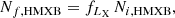
One can use the cumulative XLF to check if the systems in the observational and synthetic populations have similar distributions. From the top to the bottom of Fig. 1 we plot the observational XLF (red stars) and the synthetic XLF (solid black line) for Models 1–3 accordingly. The shape of Model 1 and Model 2 XLFs is alike but the excess of the synthetic LMXBs in Model 1 causes its XLF to be shifted toward higher numbers on the vertical axis and larger luminosities on the horizontal axis. The higher number of HMXBs in the XRBs population and more luminous IMXBs in Model 3 than in Models 1 and 2 cause its XLF slope to be shallower up to the luminosity ∼4.0 × 1038 erg s−1 and steeper above that luminosity than in the standard models.
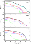 |
Fig. 1. Cumulative XLF of XRBs for M83: observations (red stars) and Model 1 (top panel), Model 2 (middle panel), and Model 3 (bottom panel). On the vertical axis is shown the number of XRBs that have a luminosity, LX, higher than the corresponding LX value on the horizontal axis. The models are plotted with solid black lines (all XRBs) and subdivided into four subcategories shown with dashed lines: HMXBs (magenta), IMBXs (blue), persistent LMXBs (cyan), outbursting transient LMXBs (green) in Model 1, or randomly selected 30 LMXBs (green) in Models 2 and 3. Model 2 is consistent with the observations in terms of the total number of XRBs and the shape of the XLF. Model 3 is close to the observations in terms of the total number of XRBs but the slope of XLF is shallower in the range log LX ∼ 36.6 − 38.6 erg s−1 than in Models 1 and 2. |
6.2.2. The number of binaries
The number of present-day XRBs is Ni = 50 834 in Model 1, Ni = 71 164 in Model 2, and Ni = 75 854 in Model 3. In each of three models, about ∼27% of the binaries have luminosities above 1035 erg s−1. Following the reduction steps described in Sect. 5 we get the synthetic population of the observable XRBs, Nf,XRBs, consisting of 819 binaries in Model 1, 1130 binaries in Model 2, and 1269 binaries in Model 3.
We decomposed XRB populations into HMXBs, IMXBs, outbursting T-LMXBs, and P-LMXBs and analysed how each of those contributes to the total XLF. From the example of Model 1, it appears that the main culprits of the mismatch between the observations and the simulations are P-LMXBs (dashed cyan line in the top panel of Fig. 1), which are too numerous (441) and brighter than observed XRBs. There is also a small overabundance of outbursting T-LMXBs (dashed green line in the top panel of Fig. 1) at luminosities, log LX ∈ [35 − 35.5] erg s−1. The number of outbursting T-LMXBs in Model 1 is 248. We chose to make one more reduction step (in addition to the reduction factors from Sect. 5) in Models 2 and 3: we drew 30 LMXBs from the set consisting of P-LMXBs and outbursting LMXBs. As a result, the final number of XRBs in Models 2 and 3 is 197 and 263, respectively, compared to 214 observed. The resulting XLFs are presented in the middle and bottom panel of Fig. 1.
6.2.3. The number of binaries in XRB subgroups
What distinguishes Model 2 (presented in the middle panel of Fig. 1) from Models 1 and 3 and makes it our model of choice is not only the total number of XRBs but also the number of different types of XRBs that closely correspond to what is observed. From Model 2 we get 30 LMXBs, 51 IMXBs, and 116 HMXBs compared to 30 LMXBs, 64 IMXBs, and 120 HMXBs observed. Although there are 30 LMXBs and 64 IMXBs in Model 3, which matches perfectly the observations, the number of synthetic HMXBs (169) exceeds the observed number by ∼41%.
6.2.4. The properties of synthetic XRBs
To shed more light on our results, we show the basic characteristic of XRB populations in Model 1, 2, and 3. The distributions of the donor masses are right-skewed in all three models (see magenta, light green and light blue boxes in the left panels of Fig. 2). The upper quartile of Mdonor distribution in Model 1 is ∼1.84 M⊙ while it is ∼15.96 M⊙ and ∼16.54 M⊙ in Models 2 and 3, respectively. This clearly demonstrates the drastic reduction of LMXBs to 30 systems in Models 2 and 3.
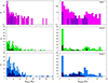 |
Fig. 2. Distributions of the donor (left column) and compact object (NS or BH; right column) masses at the onset of the XRB phase in the three models described in Sect. 6.1. The darker colors on each panel correspond to the distributions of masses of XRBs that become merging DCOs generated in ten runs for each model, as is described in Sect. 7.3. It means that the distributions for merging DCO progenitors are ten times overestimated with respect to the distributions of the other XRBs in the figure to show which part of the parameter space they occupy. |
The distribution of the compact object (NS/BH) masses has a peak at MNS/BH = 1 − 2 M⊙, corresponding to the NS type of the accreting object. The NSs constitute ∼77% of the accretors in Model 1 but in Model 2 the proportion between NSs and BHs is more balanced (∼41% NSs and ∼59% BHs), while in Model 3 the NS/BH ratio is reversed compared to Model 1 with ∼27% NSs and ∼73% BHs. The delayed SN model that we use in our evolution calculations (see Sect. 4) results in compact objects present in the so-called “mass gap” (∼2 − 5 M⊙) in the MNS/BH distribution of all three models.
In Fig. 3 we show the dependence between the donor mass, orbital period, and eccentricity of XRBs in each model. The distribution of the systems along the vertical axis mirrors our definition of LMXBs, IMXBs, and HMXBs: LMXBs (open circles) lie in the part of the diagrams where Md < 3.0 M⊙ for Model 1 and Md < 3.5 M⊙ for Models 2 and 3, all HMXBs (open squares) occupy the upper part of the diagram where Md > 8.0 M⊙, and IMXBs (open diamonds) lie in between. The maximum donor mass reaches 60 M⊙ in Models 1 and 2 and increases to ∼70 M⊙ in Model 3. The orbital periods of all LMXBs in Models 2 and 3 are shorter than ∼10 days going down to an order of minutes, while in Model 1 there are four systems with orbital periods ∼100 days. Both IMXBs and HMXBs span a wide range of Porb, from hours up to ∼3 × 10⁶ days. Systems with donors more massive than 3.5 M⊙ and wider orbits (Porb > 100 d) may also be highly eccentric; however, most of them have eccentricities below 0.4. All LMXBs have circular orbits, which is an outcome of the combined effect of the tidal circularization and CE phase that they undergo during their prior evolution. This figure is complemented by Fig. 4, which illustrates the initial orbital periods and eccentricities of the XRB progenitors at ZAMS. Fig. 4 is discussed in detail in Sects. 7.2 and 7.3.
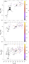 |
Fig. 3. Dependence between donor mass (M⊙), orbital period (days), and eccentricity of XRBs for all three models. The eccentricity is color coded and the open symbols represent the population of XRBs described in Sects. 6.2.2 and 6.2.3: HMXBs are plotted as open squares, IMXBs as open diamonds, and LMXBs as open circles. The crosses are XRBs that become merging DCOs generated in ten runs for each model, as is described in Sect. 7.3. It means that the DCO progenitors are ten times over-represented with respect to other XRBs in the plots to show which part of the parameters space they occupy. |
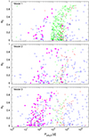 |
Fig. 4. Dependence between initial orbital period (days) and eccentricity of the XRB progenitors in Models 1 (top), 2 (middle) and 3 (bottom). The HMXB progenitors are marked as open blue squares, IMXBs are open red diamonds, and LMXBs are open green circles. The filled magenta circles are the progenitors of XRBs that become merging DCOs generated in ten runs for each model, as is described in Sect. 7.3. It means that the DCO progenitors are ten times over-represented with respect to other XRBs on the plots to show which part of the parameters space they occupy. |
6.3. Merging DCOs
We followed the future evolution of three models: the reference Model 1, the best observations matching Model 2, and the model with alternative CE development criteria (Model 3) to see if any of them produces the potential LVK sources. For each model we iterated the calculations ten times to see how the resulting number of merging DCOs changes due to the different subsets of present-day XRBs drawn from the entire XRB population by the Monte Carlo method incorporated in cmttStarTrack. We conclude that the average number of merging DCOs per population of XRBs that can be observable in M83 is on average ∼1.9 for the two standard models and 6.2 for Model 3. Specifically in the model of choice (Model 2) the average number of merging DCOs is 2.0, where BH-NS mergers contribute the most (0.8 mergers on average) and NS-NS and BH-BH make an equal contribution of 0.6 mergers of each type (see Table A.2). HMXBs are the progenitors of 1.2 mergers; of them, 0.5 are BH-BH mergers, 0.2 are BH-NS mergers, and 0.5 are NS-NS mergers. The remaining 0.8 merging binaries originate from IMXBs (0.6 are BH-NS, 0.1 are BH-BH, and 0.1 are NS-NS mergers). As a consequence of the reduction of almost all LMXBs, none of the merging DCOs in Model 2 comes from LMXBs. However, as can be seen from the results of Model 1 (see Table 2), LMXBs may be potential progenitors of merging NS-NS and BH-NS binaries. In Model 1, which contains a much larger population of LMXBs than Models 2 and 3, we find on average 1.0 NS-NS, 0.57 BH-NS, and 0.14 BH-BH mergers. Both LMXBs and IMXBs account for 0.7 of merging DCOs progenitors in Model 1, while HMXBs account for the remaining 0.3 mergers.
The higher number of HMXBs and IMXBs in Model 3 than in the standard Models 1 and 2 has its effect on the number and type of merging DCOs. We find 3.22 BH-BHs, 2.44 BH-NSs, and 0.56 NS-NSs among an average of 6.22 mergers in Model 3. All merging BH-BHs and NS-NSs have HMXBs as their progenitors. 0.88 merging BH-NSs are the result of HMXBs evolution as well, but the majority of merging BH-NSs (1.56) go through an IMXB phase in their prior evolution. In other words, HMXBs and IMXBs are the progenitors of 4.7 and 1.5 merging DCOs in Model 3.
In Fig. 2 we show the donor mass and NS/BH mass distributions of all XRBs that become merging DCOs (dark violet boxes for Model 1, dark green boxes for Model 2, and dark blue boxes for Model 3). We chose to present XRBs that become merging DCOs that we found in all ten iterations for each model, as is mentioned at the beginning of this section, to give a better view of the parameter space that they take up. Therefore, their number is represented ten times as much as XRBs that do not become merging DCOs shown in Fig. 2 in light colors.
7. Discussion
7.1. The synthetic number of XRBs
The XLFs of the synthetic populations of XRBs that we generated with the standard models (i.e., with the standard CE development criteria) have shapes that track the shape of the observational curve (see Fig. 1 for Models 1, 2). It means that for the models with standard CE development criteria the XLF shape itself of this particular XRB population (in M83) is not a good indicator of the underlying XRB population: the population that is dominated by LMXBs (689 LMXBs out of a total of 819 XRBs in Model 1) has almost the same shape as the population dominated by HMXBs (116 HMXBs out of a total of 197 XRBs in Model 2).
However, the shape of the XLF generated with the revised CE development criteria differs from the observational Model 1 and Model 2 XLFs: its slope is less steep up to the luminosity LX ∼ 4.0 × 1038 erg s−1. What can be noticed is a significant difference in the shape of IMXBs XLF (dashed blue lines in Fig. 1) between Model 3 and the other two models: IMXBs’ XLF in Model 3 does not drop at a luminosity of ∼6.0 × 1037 erg s−1 but it extends further up to LX ∼ 1.0 × 1039 erg s−1.
The higher number of luminous IMXBs in Model 3 is a result of the alternative CE development criteria adopted, which allow the systems to evolve through the stable RLOF evolutionary channel. The binaries that would merge during the CE phase initiated by the expanding, more massive star evolving in the Hertzsprung gap in the case of the standard models, go through the stable RLOF instead and after the first SN they form IMXBs with higher donor and accretor masses and higher luminosities than IMXBs formed through the CE channel, that is, there are more IMXBs with donors close to the upper donor mass limit formed.
In the case of HMXBs, their XLF shapes are alike for all three models. The evolution through the stable RLOF channel has an effect in the shift of HMXBs’ XLF toward higher numbers on the y axis. The shape of HMXBs’ XLF in Model 3 is not as much affected by the CE development criteria as IMXBs’ XLF because the criteria affect HMXBs in their whole donor mass range.
Our main modeling issue was to match the numbers of XRBs observed in M83. Typical model numbers that we find are much too large for LMXBs and somewhat too low for IMXBs and HMXBs (see Model 1 in Table 2). We checked that changing Z within the range observed in M83 does not have much influence on the synthetic XRBs population. For Z = 0.01, 0.02, 0.025, 0.03 the total number of systems differs at most by a factor of 1.3.
Apart from the CE development criteria, the number of HMXBs in our simulations is influenced the most by the slope of the IMF for massive stars and the SFR, within the small set of parameters that we varied. The uncertainty of the IMF slope for the high-mass stars, is: α3 = −2.3 ± 0.7 (Kroupa 2001). Changing α3 = −2.3 (Model 1: 75 HMXBs and 55 IMXBs) to α3 = −1.9 generates more massive stars, and thus more HMXBs and IMXBs (227 HMXBs and 225 IMXBs). It is apparent that just with a change in the IMF slope within its uncertainty we can easily match the number of observed HMXBs (120) and IMXBs (64) in M83.
As is mentioned in Sect. 4, we tested four values of SFR (1.5, 2.0, 2.5, 3.5, M⊙ yr−1). Only the models with a SFR = 3.5 M⊙ yr−1, a standard IMF slope, and a Z = 0.01 (e.g., Model 2) produce the number of HMXBs (116) approaching the observations (120). The lower the SFR, the fewer HMXBs are formed in simulations; for example, for the model with SFR = 2.5 M⊙ yr−1 and Z = 0.01 (Model 1), their number drops to 75.
From the discussion above, it is apparent that finely tuning either of the two parameters (SFR or α3) leads to the desired result considering HMXBs. However, there are other observations that motivate the specific choice of SFR that adjusts the number of HMXBs. Grimm et al. (2003) inferred the relation between the SFR and the total number, N, of HMXBs with luminosities LX > 2.0 × 1038 erg s−1 from the observations of 14 local galaxies:
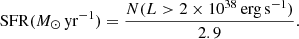
This relation predicts that for SFR = 3.5 M⊙ yr−1 the number of luminous HMXBs should be N ∼ 10. Our model with SFR = 3.5 M⊙ yr−1, α3 = −2.3, and Z = 0.01 (Model 2) gives nine such systems. Equation (6) predicts only N ∼ 7 for SFR = 2.5 M⊙ yr−1 while we find 17 such binaries in the model where SFR = 2.5 M⊙ yr−1, α3 = −1.9, and Z = 0.01.
We did not consider transient IMXBs or HMXBs with Be-star or Oe-star donors (Oe/Be-XRBs) in the models. Some of our XRBs with normal O/B star donors (core H-burning) can be Oe/Be-XRBs, and they should be removed from our model populations if they are in quiescence. The quiescence luminosity of these systems is LX ≤ 1.0 × 1033 erg s−1 (e.g. Negueruela 2010), which is below the Chandra detectability limit for M83. We made a rough estimation of how many HMXBs should be considered quiescent in our model of choice (Model 2) following the assumptions in Belczynski & Ziolkowski (2009): there are ten systems out of 116 HMXBs that have companions burning H in their core, and assuming that only 25% of them are Be-XRBs (e.g. McSwain 2005) and that their DC is 10 − 30% (Belczynski & Ziolkowski 2009), at most one of them is a quiescent Be-XRB. Excluding them from our sample would have little influence on our conclusions, but it would also imply that the number of HMXBs in a given model is an upper limit.
While the agreement between the observational and synthetic number of HMXBs in models with SFR = 3.5 M⊙ yr−1, α3 = −2.3, and Z = 0.01 is satisfying, the number of IMXBs is still too high (95 compared to 64 observed). This was the motivation to look closer at the mass limits adopted in the classification of XRBs into three groups (see Sect. 2). The mass limits taken from the comparison of the optical observations to evolutionary tracks in H21 are accurate to 1.0 M⊙ due to the fact that stellar evolution tracks are probed every 1.0 M⊙. Therefore, the stars of a mass below 3.5 M⊙ may be classified as 3.0 M⊙ stars. It appears that, in the sample of 95 IMXBs, 44 have secondaries with masses in the range 3.0 M⊙ < M2 < 3.5 M⊙. Changing the condition for the maximum mass of the donor in LMXBs from M2 < 3.0 M⊙ to M2 < 3.5 M⊙ lowers the number of IMXBs to 51 and brings it closer to the number derived from the observations.
The main problem for us to solve is the striking excess of LMXBs produced in the simulations (689 in Model 1) in comparison to only 30 LMXBs identified in M83. LMXBs are subdivided into two major categories – persistent LMXBs (441 in Model 1) and transient LMXBs in outburst (248 in Model 1 – as quiescent transients are not bright enough to make the Chandra detection threshold). The division between transient and persistent LMXBs strongly depends on the disk stability limits determined by the disk instability model (see Sect. 5.3). Although the adopted model is successful at predicting the transient or persistent nature of observed LMXBs (Lasota et al. 2008; Coriat et al. 2012), the “model calibration” (see parameter Cirr in Eqs. (4) and (5)) is still highly uncertain. One could think of shifting as many P-LMXBs into the T-LMXB category, and then removing them by putting some of them in quiescence (too low a luminosity to make the Chandra threshold for the observation dataset that we employ). However, we have already adopted the lower limit on Cirr = 0.001 (Tetarenko et al. 2018) minimizing the number of P-LMXBs. Higher Cirr leads to a decrease in the critical accretion rate above which LMXBs become persistent X-ray sources, which results in more P-LMXBs in our synthetic populations.
It was noted that for LMXBs with a very low donor to accretor mass ratio (q ≤ 0.02) the disk stability criteria presented in Sect. 5.3 may not work due to tidal forces operating on the accretion flow (Yungelson et al. 2006). However, as was pointed out by Lasota et al. (2008), the maximum outburst luminosities inferred from the adopted disk model (Eq. (4)) for helium ultracompact X-ray binaries are consistent with observations, which indicates that the adopted model works, at least for some very low mass ratio LMXBs.
In the case of T-LMXBs, the number of systems in outburst is defined by the adopted DC: 2.5% of time spent in outburst Yan & Yu (2015). The DC is subject to large uncertainties and spans the range 0.9 − 7% (see also Sect. 5.3). By lowering the DC from 2.5% to 0.9% we can lower the fraction of the “visible” T-LMXBs in the outburst in our models (e.g., from 248 to 89 for Model 1). But this hardly improves the issue. To agree with the observations, we removed (manually) all but 30 randomly chosen LMXBs from our synthetic populations (Models 2 and 3). By choosing randomly 30 LMXBs, we admit that we are not able to reproduce even such a basic property of the LMXB population as the number of LMXB sources observed in a well-known nearby galaxy. This failure must lead to future study of the evolutionary processes that are important factors in the formation of LMXBs (mass transfer events in close binaries, natal kicks received by compact objects, and magnetic braking, among other uncertain evolutionary factors).
7.2. XRBs characteristic
The XRBs in the synthetic population form from the binaries that have a wide range of initial orbital periods and eccentricities, as can be seen in Fig. 4. The HMXB progenitors are widely scattered in the parameter space in all three models, the LMXB progenitors cluster within the narrow range of the orbital periods, Porb, 0 ∼ 8.0 × 10² − 2.0 × 10⁴ days, and the IMXB progenitors follow the orbital period range similar to LMXB progenitors in Models 1 and 2, but they can also have orbital periods in the range ∼10 − 200 days in Model 3. These constraints on the orbital period ranges come from the subsequent evolution that the binaries have to follow to form XRBs (see below).
The orbital parameters of the formed XRBs are shaped by:
-
(i)
The assumed criteria of CE development.
-
(ii)
The mass loss of the massive stars due to their stellar winds, which widens the orbit and changes the mass ratio of the binary.
-
(iii)
The natal kick that the system encounters during a SN explosion, which randomly changes the eccentricity and orbital separation of the binary.
-
(iv)
The time period during which the tides between the binary components may act to circularize the orbit.
The interplay between these factors results in the population of XRBs plotted in open symbols in Fig. 3 for all three models.
The impact of different CE development criteria applied in Models 1 and 2 and Model 3 on HMXB and IMXB populations can be seen when one compares Figs. 4 and 3. This is because the systems that would undergo CE phase and merge in Model 1(2) go through a stable mass transfer and survive as HMXBs or IMXBs in Model 3. LMXBs are insensitive to the revised CE development criteria from the definition of the latter given in Sect. 4. Their progenitors have to have orbital periods on the order of 103 days to survive the subsequent evolution. They form LMXBs with orbital periods shorter than two days. The LMXB progenitors have all range of eccentricities but the circularization of an orbit, which is an interplay between the tides and the Roche lobe overflow mass transfer and which takes place in the LMXB phase, causes all synthetic LMXBs to have e = 0.
7.3. Merging DCOs
To better present the characteristic of XRBs that form merging DCOs we present separately all such XRBs from ten different subsets of the present-day XRBs in M83 drawn from the entire XRBs population as dark histograms in Fig. 2 and filled circles in Figs. 3 and 4 (we do not present the whole present-day XRBs population from all ten runs for clarity of Fig. 3). It means that the progenitors of merging DCOs are ten times over-represented in all those figures. Although it may be visually misleading, our purpose is to show which part of the parameter space is occupied by such systems. The densely populated part of the top panel of Fig. 3 is zoomed in on in Fig. A.1.
As can be seen in Fig. 4, most of the progenitors of XRBs that form merging DCOs (filled magenta circles) span the whole range of initial eccentricities but the values of their initial orbital periods, Porb, 0, are tightly connected to the criteria for the CE development that are applied in their subsequent evolution: most of them have Porb, 0 in the range between tens to hundreds of days in Model 3, while there are progenitors that have much longer periods on the order of a few thousand days in Models 1 and 2. The orbit of the merging DCO progenitors cannot initially be too wide in Model 3 because most of the merging DCO progenitors evolve through the stable mass transfer channel and the shrinkage of their orbit will not be as dramatic as during the CE phase, which is a dominant evolution channel for merging DCOs in Models 1 and 2. All merging DCOs in our ten samples of each model form from XRBs with orbital periods lower than ∼2 × 10³ days. In Models 1 and 2, the merging DCO progenitor group at the two orbital period ranges: the short period range from ∼2.4 h to a few days and the long period range around 103 days. There are no merging DCO progenitors with orbital periods in between. In the long orbital period group there are only XRBs with high-mass donors; in other words, these are the systems that become XRBs due to the wind accretion before they undergo the CE phase. All systems in the short group become XRBs after the CE. In the model with the revised CE development criteria (Model 3) the XRBs resulting in merging DCOs are more evenly distributed; however, most of them still have Porb ∼ 2 h to ∼2 days. The lack of a gap in the orbital period distribution in Model 3 illustrates the characteristic feature of this model: there exist systems that undergo the stable mass transfer rate shrinking their orbit gradually in the regime not available for the merging DCO progenitors in Models 1 and 2.
There are only a few systems that we find in the population of merging DCOs becoming XRBs in our ten runs that have eccentric orbits: two in Model 1, one in Model 2, and seven in Model 3. All these systems are HMXBs in which tidal forces have not yet circularized the orbit at the time that they become wind-fed XRBs.
The merging DCOs constitute ∼1% (Models 1 and 2) to ∼2% (Model 3) of the intrinsic XRB population in M83. The dominant merging DCO type depends on the model: it is NS-NS in Model 1, BH-NS in Model 2, and BH-BH in Model 3 (see Table A.2). At this point we can also compare the fraction of HMXBs that will merge as BH-BH in each model with the expectations inferred by Liotine et al. (2023). They estimate that ∼0.6% of detectable HMXBs will merge as BH-BH within the Hubble time. From our synthetic population of HMXBs detectable in M83 we find that ∼0.22%, ∼0.43%, and ∼1.89% of such systems will merge as BH-BH in Models 1, 2, and 3, respectively. The number from Model 2 is the closest to the estimations of Liotine et al. (2023), which adds to the arguments in favor of Model 2 being the model of choice.
In the models in which we reduce the number of LMXBs to 30 systems (Models 2 and 3) the most probable progenitors of merging DCOs are HMXBs, but in the model in which P-LMXBs and outbursting T-LMXBs are not arbitrarily removed (Model 1) the population of LMXBs contributes to the number of merging DCOs to the same extent as the population of IMXBs (see Table 2). However, the probability that LMXBs will evolve into a merging NS-NS is much lower than for IMXBs or HMXBs in Model 1: only 1 in 1000 LMXBs may result in a merging DCO comparing to 12 in 1000 IMXBs and 4 to 1000 HMXBs. Assuming the same effectiveness of merging DCO production from LMXBs in Models 2 and 3, we estimate that from 30 LMXBs we can expect ∼0.03 mergers in those models.
Regarding the uncertainty that we have about the LMXBs evolution, we cannot exclude the possibility that ∼1 LMXB forming merging DCO does not appear in the population of LMXBs in Models 2 and 3 only due to our artificial selection of 30 systems. We have no means to tell if the population of observable LMXBs in M83 contains or does not contain the system that will merge as NS-NS in the future. To assess the consequences of our approach to LMXBs in Models 2 and 3, let’s assume that 30 LMXBs in Model 2 or 3 drawn in ten runs give 0.7 (at most) merging DCOs, like in Model 1. This assumption is equivalent to the situation when 30 LMXBs would have been drawn from the part of the LMXB parameter space that is most likely to result in a merging DCO. This changes the expected number of merging DCOs by ∼24.8% (from 2.03 to 2.70) in Model 2 and by ∼9.7% in Model 3 (from 6.23 to 6.90). The change in the number of merging DCOs is not negligible, especially in Model 2, but it does not influence our conclusions.
In all three models, merging BH-BHs come from HMXBs with accreting BHs (BH-HMXBs). The typical evolution leading to a merging BH-BH starts with the binary composed of two massive stars. When the initially more massive star (primary) ends to burn hydrogen in its core, its expansion leads to thermal time-scale mass transfer (TTMT) on the less massive star (secondary), which is still in the main sequence. The primary loses almost its entire hydrogen envelope in the process, which inhibits its rapid expansion. The mass transfer ceases when the radius of the primary Roche lobe becomes larger than the radius of the primary itself. As the evolution of the donor proceeds, it becomes a naked He-star, which forms the first BH, and the system becomes a wide BH-MS binary. Soon after the secondary evolves into the core He-burning star (CHeB) its radius surpasses its Roche lobe radius. Depending on the CE development criteria adopted in the model, the future evolution of the BH-CHeB binary may go through two different channels leading to the final merger: the CE channel (the standard criteria in Models 1 and 2, Belczynski et al. 2008) or the stable RLOF channel (the alternative criteria in Model 3, Olejak et al. 2021).
In the CE channel, the BH-CHeB goes through the CE and the donor becomes the naked He-star. The system becomes a HMXB that lives for ∼1.0 Myr. In subsequent evolution, the system survives the second SN explosion, becoming a tight BH-BH binary that merges within the Hubble time. In the stable RLFO channel, after the first BH is formed, the second star leaves the main sequence, expands, and initiates TTMT onto BH, but here the alternative CE development criteria allow the system to avoid the formation of a CE. During the stable TTMT phase, all systems that form merging BH-BHs in Model 3 have a heavy donor star transferring mass onto the light BH (q ∼ 4 − 5) and their orbits shrink significantly (by about two orders of magnitude). The mass transfer ceases when the donor becomes a naked He-star and the subsequent evolution of the binary follows the same path as in Models 1 and 2, leading to the formation of a merging BH-BH.
Most merging BH-NS binaries in all three models come from IMXBs with accreting BHs (BH-IMXBs), which follow the CE evolution channel similarly to BH-HMXBs in Models 1 and 2, as is described above. The alternative CE development criteria are not fulfilled here because the donor ZAMS mass is below 18 M⊙ in these systems (see Sect. 4). After the CE phase, the donor becomes an evolved helium star. The system mass ratio is now low enough to allow for stable mass transfer into a BH and the system appears as IMXBs. Further evolution results in the second SN and NS formation. A few hundred Myrs after its formation, the binary consisting of a NS and a BH merges.
If we exclude almost all LMXBs from the population (Models 2 and 3), all merging NS-NS binaries form from HMXBs when the NS is a compact object (NS-HMXB). The evolutionary paths of NS-HMXBs are similar to those of BH-HMXBs in the same models. The difference is that when the binary goes through the CE stage the donor is already a core He-burning H-rich star, which subsequently becomes the evolved helium star. When the CE phase ends, the system is close enough for the donor to start the mass transfer onto the NS. While transferring mass, the donor proceeds onto the giant branch of He-stars. If the system survives the subsequent SN explosion and its orbital separation is sufficiently small, it ends up as a merging NS-NS.
In the model where all outbursting T-LMXBs and P-LMXBs are included (Model 1) the population of LMXBs may have a non-negligible contribution to the number of the progenitors of the merging NS-NS (see Table 2 and discussion above in this section). Such systems can form from LMXBs when the donor to the firstborn NS is a helium star with the mass 2.6 ≤ M ≤ 6.7 M⊙ (Belczyński & Kalogera 2001; Dewi et al. 2002). In the typical evolution of LMXBs into the merging NS-NS in Model 1, the more massive main sequence star evolves into a Hertzsprung gap star where its rapid expansion leads to TTMT. When the mass ratio reverses and the initially more massive primary loses almost 50% of its mass, the mass transfer changes from TTMT to nuclear RLOF, during which the mass is transferred from the less massive to the more massive binary component. When the mass transfer stops, the primary is a red giant star. Finally, it becomes an evolved helium star that explodes as a SN, leaving a NS behind. The evolution of the secondary proceeds. It becomes a red giant that at some point initiates the CE phase, resulting in a NS-naked He-star binary on an orbit of a few solar radii. Then the expanding He-star initiates the second episode of TTMT. While transferring mass, the secondary evolves into an helium giant branch star that turns into a NS after a second SN event. The NS-NS binary that forms merges within a few hundred Myrs.
The evolutionary paths of the systems leading to merging DCOs in our simulations are given in Tables C.1 and C.2, and the schematic pictures of the typical evolution of a merging BH-BH from an HMXB, a NS-BH from an IMXB, and a NS-NS from an LMXB in Model 1 are included in Appendix C.
To understand the scarcity of the merging DCOs in the synthetic population, we followed the evolutionary paths of HMXBs, IMXBs, and LMXBs that do not form merging DCOs. We give the numbers for the model of choice (Model 2) but the described evolution is valid in all three models.
There are four typical evolutionary paths that prevent the formation of a merging DCO from an HMXB. Among all the HMXBs that do not end up as merging DCOs:
-
a)
More than half (∼56.7%) are formed as wide binaries with a core-helium hydrogen-rich giant donor, where the accretion takes place through the stellar wind. A wide orbit means that the binding energy of the binary is small and as a result most of these systems are disrupted after the SN explosion of the secondary.
-
b)
∼24.3% remain bound with two compact objects orbiting each other but their separation (on the order of a few thousand R⊙) is too large for the merger to appear within the Hubble time.
-
c)
∼11.7% (only the ones with a NS) go through the CE and tighten their orbits to tens of R⊙ but the natal kicks imparted to the newly formed NS after the second SN are strong enough to disrupt these systems.
-
d)
The remaining ∼7.3% form HMXBs with a main-sequence donor after the first SN and with small-enough orbital periods that they merge when the donor becomes a low-mass He-giant and initiates the CE phase.
In the population of IMXBs that do not merge as DCOs in their final stage of evolution, almost all BH-IMXBs end up as wide, noninteracting binaries where the companion star is a CO white dwarf (WD) and just a few percent of BH-IMXBs are disrupted after the second SN, which leads to the birth of the second BH. The final fate of NS-IMXBs is more diversified: (i) the majority become close binaries but with a merging time well beyond Hubble time. Among them about one half are NS-NS binaries and the second half are NS-WDs (CO or ONe WD); (ii) some form NS-hybrid WD systems that eventually merge and (iii) a few of the systems fall apart after the creation of the second NS.
In Model 1 almost all the LMXBs that do not form merging DCOs end their lives either as a NS-NS or WD-NS, which do not merge in Hubble time, or as binaries where the companion star merges with a NS/BH before it becomes a compact object.
In this work we consider only the isolated binary evolution scenario. Among alternative scenarios for the evolution of the progenitors of merging DCOs, the most widely considered is the scenario of dynamical interactions in dense stellar clusters. The question may arise of whether the XRBs from the dynamical interactions could have contributed to the observed XRB population in M83. However, the numerical simulations that investigate the possible population of dynamically formed XRBs in the Milky Way show that it is unlikely that they significantly contribute to the observed population of LMXBs (Kremer et al. 2018). High-mass X-ray binaries follow the regions of higher SFR and there is some evidence that they may be associated with young stellar clusters (Kaaret et al. 2004; Garofali et al. 2012) that can be found in the same regions. But though HMXBs may be born in such clusters, the simulations done for HMXBs in NGC 4449 show that it is very unlikely that they were formed dynamically (Garofali et al. 2012). We assume that these conclusions also apply to M83.
8. Conclusions
We performed numerical simulations on a nearby galaxy, M83, to reproduce its X-ray binary populations and predict its capacity to form merging DCOs (sources of gravitational waves) out of these X-ray binaries. We find that:
-
We can match the shape of the observed X-ray luminosity function, the number of XRBs, and their specific subcategories (LMXBs, IMXBs, and HMXBs) for the evolutionary channel that allows for the effective formation of merging DCOs through CE evolution (Model 2). However, this match can be obtained only with a drastic artificial reduction of LMXBs in our synthetic population. This shows that the physics involved in the formation of LMXBs is not well understood and requires further in-depth investigation. Also, it is argued that our standard CE development criteria may be too optimistic in light of recent detailed evolutionary studies.
-
The evolutionary model in which the majority of merging DCO formation occurs with the help of stable RLOF (without the assistance of a CE; Model 3) does not provide a good match to the observed XLF shape. However, we note that this model is rather extreme and restrictive in its assumptions on CE development criteria. Possibly, a more realistic model that can form merging DCOs through CE and stable RLOF (something between Model 2 and 3) in more balanced proportions is required in future studies.
-
Independently of our adopted evolutionary scenario, only ∼1 − 2% of M83 XRBs will form merging DCOs. This comes from the fact that evolution terminates X-ray binaries in binary component interactions, binary disruptions at second SN, or leads to the formation of wide (non-merging) DCOs.
Our conclusions are not a general statement about XRBs and their merging DCO production efficiency, but apply only to this specific galaxy with a rather high metallicity. Yet, most of local galaxies for which X-ray observations exist do typically have a high metallicity. Despite the fact that the connection between local XRBs and merging DCOs is rather weak, studies of XRB populations may help to constrain the uncertain evolutionary physics that is involved in the formation of LIGO-Virgo-KAGRA sources.
Acknowledgments
We thank the anonymous referee for their useful suggestions and comments that helped to improve this paper. This work was supported by the Polish National Science Center (NCN) grant Maestro (2018/30/A/ST9/00050). I.K. would like to thank Aleksandra Olejak, Amedeo Romagnolo and Alex Gormaz-Matamala for valuable discussions and comments.
References
- Abbott, R., Abbott, T. D., Acernese, F., et al. 2023, Phys. Rev. X, 13, 041039 [Google Scholar]
- Anastasopoulou, K., Zezas, A., Steiner, J. F., & Reig, P. 2022, MNRAS, 513, 1400 [NASA ADS] [CrossRef] [Google Scholar]
- Antonini, F., & Perets, H. B. 2012, ApJ, 757, 27 [NASA ADS] [CrossRef] [Google Scholar]
- Belczyński, K., & Kalogera, V. 2001, ApJ, 550, L183 [CrossRef] [Google Scholar]
- Belczynski, K., & Ziolkowski, J. 2009, ApJ, 707, 870 [NASA ADS] [CrossRef] [Google Scholar]
- Belczynski, K., Kalogera, V., & Bulik, T. 2002, ApJ, 572, 407 [NASA ADS] [CrossRef] [Google Scholar]
- Belczynski, K., Taam, R. E., Kalogera, V., Rasio, F. A., & Bulik, T. 2007, ApJ, 662, 504 [Google Scholar]
- Belczynski, K., Kalogera, V., Rasio, F. A., et al. 2008, ApJS, 174, 223 [Google Scholar]
- Belczynski, K., Bulik, T., Fryer, C. L., et al. 2010, ApJ, 714, 1217 [NASA ADS] [CrossRef] [Google Scholar]
- Belczynski, K., Klencki, J., Fields, C. E., et al. 2020, A&A, 636, A104 [NASA ADS] [CrossRef] [EDP Sciences] [Google Scholar]
- Blair, W. P., Chandar, R., Dopita, M. A., et al. 2014, ApJ, 788, 55 [NASA ADS] [CrossRef] [Google Scholar]
- Bresolin, F., Schaerer, D., González Delgado, R. M., & Stasińska, G. 2005, A&A, 441, 981 [NASA ADS] [CrossRef] [EDP Sciences] [Google Scholar]
- Bresolin, F., Ryan-Weber, E., Kennicutt, R. C., & Goddard, Q. 2009, ApJ, 695, 580 [Google Scholar]
- Bruzzese, S. M., Thilker, D. A., Meurer, G. R., et al. 2020, MNRAS, 491, 2366 [NASA ADS] [CrossRef] [Google Scholar]
- Clesse, S., & García-Bellido, J. 2022, Phys. Dark Universe, 38, 101111 [NASA ADS] [CrossRef] [Google Scholar]
- Coriat, M., Fender, R. P., & Dubus, G. 2012, MNRAS, 424, 1991 [NASA ADS] [CrossRef] [Google Scholar]
- De Luca, V., Desjacques, V., Franciolini, G., & Riotto, A. 2020, JCAP, 2020, 028 [CrossRef] [Google Scholar]
- de Mink, S. E., & Belczynski, K. 2015, ApJ, 814, 58 [Google Scholar]
- Dewi, J. D. M., Pols, O. R., Savonije, G. J., & van den Heuvel, E. P. J. 2002, MNRAS, 331, 1027 [CrossRef] [Google Scholar]
- Eldridge, J. J., & Stanway, E. R. 2016, MNRAS, 462, 3302 [Google Scholar]
- Fragione, G., Grishin, E., Leigh, N. W. C., Perets, H. B., & Perna, R. 2019, MNRAS, 488, 47 [NASA ADS] [CrossRef] [Google Scholar]
- Fragos, T., Lehmer, B., Tremmel, M., et al. 2013, ApJ, 764, 41 [NASA ADS] [CrossRef] [Google Scholar]
- Fragos, T., Andrews, J. J., Bavera, S. S., et al. 2023, ApJS, 264, 45 [NASA ADS] [CrossRef] [Google Scholar]
- Fryer, C. L., Belczynski, K., Wiktorowicz, G., et al. 2012, ApJ, 749, 91 [Google Scholar]
- Garofali, K., Converse, J. M., Chandar, R., & Rangelov, B. 2012, ApJ, 755, 49 [NASA ADS] [CrossRef] [Google Scholar]
- Ge, H., Webbink, R. F., & Han, Z. 2020, ApJS, 249, 9 [NASA ADS] [CrossRef] [Google Scholar]
- Grimm, H. J., Gilfanov, M., & Sunyaev, R. 2003, MNRAS, 339, 793 [Google Scholar]
- Hamann, W. R., & Koesterke, L. 1998, A&A, 335, 1003 [Google Scholar]
- Hameury, J. M. 2020, Adv. Space Res., 66, 1004 [Google Scholar]
- Hobbs, G., Lorimer, D. R., Lyne, A. G., & Kramer, M. 2005, MNRAS, 360, 974 [Google Scholar]
- Hunt, Q., Gallo, E., Chandar, R., et al. 2021, ApJ, 912, 31 [NASA ADS] [CrossRef] [Google Scholar]
- Hurley, J. R., Pols, O. R., & Tout, C. A. 2000, MNRAS, 315, 543 [Google Scholar]
- Kaaret, P., Alonso-Herrero, A., Gallagher, J. S., et al. 2004, MNRAS, 348, L28 [NASA ADS] [CrossRef] [Google Scholar]
- King, A. R. 2009, MNRAS, 393, L41 [NASA ADS] [Google Scholar]
- Kremer, K., Chatterjee, S., Rodriguez, C. L., & Rasio, F. A. 2018, arXiv e-prints [arXiv:1802.04895] [Google Scholar]
- Kretschmar, P., Fürst, F., Sidoli, L., et al. 2019, New Astron. Rev., 86, 101546 [Google Scholar]
- Kroupa, P. 2001, MNRAS, 322, 231 [NASA ADS] [CrossRef] [Google Scholar]
- Kroupa, P., Tout, C. A., & Gilmore, G. 1993, MNRAS, 262, 545 [NASA ADS] [CrossRef] [Google Scholar]
- Lasota, J.-P. 2001, New Astron. Rev., 45, 449 [Google Scholar]
- Lasota, J. P., Dubus, G., & Kruk, K. 2008, A&A, 486, 523 [NASA ADS] [CrossRef] [EDP Sciences] [Google Scholar]
- Lehmer, B. D., Eufrasio, R. T., Tzanavaris, P., et al. 2019, ApJS, 243, 3 [NASA ADS] [CrossRef] [Google Scholar]
- Liotine, C., Zevin, M., Berry, C. P. L., Doctor, Z., & Kalogera, V. 2023, ApJ, 946, 4 [NASA ADS] [CrossRef] [Google Scholar]
- Lipunov, V. M., Postnov, K. A., & Prokhorov, M. E. 1997, Astron. Lett., 23, 492 [NASA ADS] [Google Scholar]
- Long, K. S., Kuntz, K. D., Blair, W. P., et al. 2014, ApJS, 212, 21 [Google Scholar]
- Lü, G. L., Zhu, C. H., Postnov, K. A., et al. 2012, MNRAS, 424, 2265 [CrossRef] [Google Scholar]
- Mandel, I., & de Mink, S. E. 2016, MNRAS, 458, 2634 [NASA ADS] [CrossRef] [Google Scholar]
- Mapelli, M. 2016, MNRAS, 459, 3432 [NASA ADS] [CrossRef] [Google Scholar]
- McSwain, M. V., & Gies, D. R. 2005, ASP Conf. Ser., 337, 270 [NASA ADS] [Google Scholar]
- Misra, D., Fragos, T., Tauris, T. M., Zapartas, E., & Aguilera-Dena, D. R. 2020, A&A, 642, A174 [NASA ADS] [CrossRef] [EDP Sciences] [Google Scholar]
- Misra, D., Kovlakas, K., Fragos, T., et al. 2024, A&A, 682, A69 [NASA ADS] [CrossRef] [EDP Sciences] [Google Scholar]
- Mondal, S., Belczyński, K., Wiktorowicz, G., Lasota, J.-P., & King, A. R. 2020, MNRAS, 491, 2747 [Google Scholar]
- Negueruela, I. 2010, ASP Conf. Ser., 422, 57 [Google Scholar]
- Olejak, A., & Belczynski, K. 2021, ApJ, 921, L2 [NASA ADS] [CrossRef] [Google Scholar]
- Olejak, A., Belczynski, K., & Ivanova, N. 2021, A&A, 651, A100 [NASA ADS] [CrossRef] [EDP Sciences] [Google Scholar]
- Olejak, A., Fryer, C. L., Belczynski, K., & Baibhav, V. 2022, MNRAS, 516, 2252 [NASA ADS] [CrossRef] [Google Scholar]
- Osaki, Y. 1974, PASJ, 26, 429 [NASA ADS] [Google Scholar]
- Pavlovskii, K., Ivanova, N., Belczynski, K., & Van, K. X. 2017, MNRAS, 465, 2092 [Google Scholar]
- Petrov, P., Singer, L. P., Coughlin, M. W., et al. 2022, ApJ, 924, 54 [NASA ADS] [CrossRef] [Google Scholar]
- Portegies Zwart, S. F., & McMillan, S. L. W. 2000, ApJ, 528, L17 [Google Scholar]
- Rodriguez, C. L., Amaro-Seoane, P., Chatterjee, S., et al. 2018, Phys. Rev. D, 98, 123005 [NASA ADS] [CrossRef] [Google Scholar]
- Sana, H., de Mink, S. E., de Koter, A., et al. 2012, Science, 337, 444 [Google Scholar]
- Sana, H., de Koter, A., de Mink, S. E., et al. 2013, A&A, 550, A107 [NASA ADS] [CrossRef] [EDP Sciences] [Google Scholar]
- Sanjurjo-Ferrín, G., Torrejón, J. M., Postnov, K., et al. 2021, MNRAS, 501, 5892 [CrossRef] [Google Scholar]
- Smak, J. 1982, Acta Astron., 32, 199 [NASA ADS] [Google Scholar]
- Stegmann, J., Antonini, F., Schneider, F. R. N., Tiwari, V., & Chattopadhyay, D. 2022, Phys. Rev. D, 106, 023014 [NASA ADS] [CrossRef] [Google Scholar]
- Tagawa, H., Haiman, Z., & Kocsis, B. 2020, ApJ, 898, 25 [NASA ADS] [CrossRef] [Google Scholar]
- Tammann, G. A., Loeffler, W., & Schroeder, A. 1994, ApJS, 92, 487 [Google Scholar]
- Tetarenko, B. E., Dubus, G., Lasota, J. P., Heinke, C. O., & Sivakoff, G. R. 2018, MNRAS, 480, 2 [Google Scholar]
- Toonen, S., Claeys, J. S. W., Mennekens, N., & Ruiter, A. J. 2014, A&A, 562, A14 [NASA ADS] [CrossRef] [EDP Sciences] [Google Scholar]
- Toonen, S., Hamers, A., & Portegies Zwart, S. 2016, Comput. Astrophys. Cosmol., 3, 6 [NASA ADS] [CrossRef] [Google Scholar]
- Tsygankov, S. S., Doroshenko, V., Poutanen, J., et al. 2022, ApJ, 941, L14 [NASA ADS] [CrossRef] [Google Scholar]
- Tzanavaris, P., Fragos, T., Tremmel, M., et al. 2013, ApJ, 774, 136 [NASA ADS] [CrossRef] [Google Scholar]
- Vigna-Gómez, A., Toonen, S., Ramirez-Ruiz, E., et al. 2021, ApJ, 907, L19 [Google Scholar]
- Vink, J. S., & de Koter, A. 2005, A&A, 442, 587 [NASA ADS] [CrossRef] [EDP Sciences] [Google Scholar]
- Vink, J. S., de Koter, A., & Lamers, H. J. G. L. M. 2001, A&A, 369, 574 [NASA ADS] [CrossRef] [EDP Sciences] [Google Scholar]
- Wang, S., Liu, J., Qiu, Y., et al. 2016, ApJS, 224, 40 [Google Scholar]
- Webbink, R. F. 1984, ApJ, 277, 355 [NASA ADS] [CrossRef] [Google Scholar]
- Xu, X.-J., & Li, X.-D. 2010a, ApJ, 722, 1985 [NASA ADS] [CrossRef] [Google Scholar]
- Xu, X.-J., & Li, X.-D. 2010b, ApJ, 716, 114 [Google Scholar]
- Yan, Z., & Yu, W. 2015, ApJ, 805, 87 [NASA ADS] [CrossRef] [Google Scholar]
- Yungelson, L. R., Lasota, J. P., Nelemans, G., et al. 2006, A&A, 454, 559 [NASA ADS] [CrossRef] [EDP Sciences] [Google Scholar]
- Yungelson, L. R., Kuranov, A. G., & Postnov, K. A. 2019, MNRAS, 485, 851 [NASA ADS] [CrossRef] [Google Scholar]
Appendix A: Additional tables and figures
Here, we present two additional tables and one figure that complement the main text. In Table A.1 we summarize the values of the reduction factors calculated for each model described in Sec. 5. In Table A.2 we distinguish the contribution of different types of merging DCOs in the total number of merging DCOs from XRBs in Models 1, 2, and 3 given in Table 2 and described in the main text in Sec. 6.3.
Reduction factors described in Sec. 5 for each of the three models.
Average number of merging DCOs of a given type in three models described in Sec. 6.1.
Fig. A.1 gives a better insight into the most clustered region in the bottom left part of the top panel (Model 1) of Fig. 3 described in Sec. 7.2 and Sec. 7.3. We show here that there are no merging DCO progenitors with Mdonor < 2.0 M⊙ and Porb days.
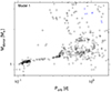 |
Fig. A.1. Zoomed-in part of the top panel (Model 1) of Fig. 3 (described in Sec. 7.2 and Sec. 7.3) where the points cluster the most. Blue crosses correspond to XRBs that form merging DCOs and open symbols show the rest of the XRB synthetic population in Model 1 (see Sec. 6.1). The figure shows that there are no XRBs that form merging DCOs with Mdonor < 2.0 M⊙ and Porb < 2.0 days. We note that the merging DCO progenitors are ten times over-represented with respect to other XRBs on the plot to show which part of the parameter space they occupy. |
Appendix B: Model 4 - the model with a rapid SN engine.
Observed and model numbers of XRBs for galaxy M83.
We checked how the model with an SN mechanism that produces the mass gap in compact objects’ mass distribution (rapid SN engine Fryer et al. 2012) changes the results compared to the three models described in the main text. There is a significant increase in the number of XRBs in Model 4 compared to Models 1-3. The quick explanation is that the BHs produced in the rapid SN model have masses above the mass gap so they are on average more massive than BHs in the delayed SN model. Hence, more BHs experience weaker natal kicks then in the rapid SN model, which allows more systems to survive (for a detailed discussion of the impact of the SN engine on the subsequent evolution of the binaries with NS/BHs, see Olejak et al. 2022). We conclude that the rapid model apparently produces even larger tension with the observations.
Appendix C: The typical evolution of XRBs that are the progenitors of merging DCOs.
We present the summary of the typical evolution paths of merging DCOs from XRBs in our models in Table C.1 and Table C.2 for Models 1 and 2 and Model 3, respectively. We also show the schematic pictures of the typical evolutionary scenarios leading to merging BH-BH from HMXB (Fig. C.3) and BH-NS from IMXB (Fig. C.2) in Models 1 and 2 and to NS-NS from LMXB (Fig. C.1) in Model 1. A more detailed description can be found in the main text in Sec. 7.3.
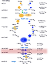 |
Fig. C.1. Typical evolution of a binary that becomes an LMXB and ends up as a merging NS-NS in Model 1. The timescale (in Myr) is shown on the left side of the panel, the masses (in M⊙) are marked next to the stars they refer to, and the orbital separation (a in R⊙) and eccentricity (e) of the system at a given stage of the evolution are shown on the right side of the panel. The acronyms on the figure stand for: MS - main sequence star HG - Hertzsprung gap star RG - first giant branch star CHeB - core helium burning star HeMS - main sequence naked helium star HeHG - Hertzsprung gap naked helium star NS - neutron star BH - black hole CE - common envelope SN - supernova explosion nRLOF - nuclear Roche lobe overflow TTMT - thermal time-scale mass transfer |
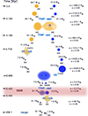 |
Fig. C.2. Typical evolution of the binary that becomes an IMXB and ends up as a merging NS-BH in Model 1. The timescale (in Myr) is shown on the left side of the panel, the masses (in M⊙) are marked next to the stars they refer to, and the orbital separation (a in R⊙) and eccentricity (e) of the system at a given stage of the evolution are shown on the right side of the panel. The acronyms on the figure are the same as in Fig. C.1. |
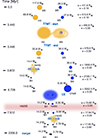 |
Fig. C.3. Typical evolution of the binary that becomes HMXB and ends up as a merging BH-BH in Model 1. The timescale (in Myr) is shown on the left side of the panel, the masses (in M⊙) are marked next to the stars they refer to, and the orbital separation (a in R⊙) and eccentricity (e) of the system at a given stage of evolution are shown on the right side of the panel. The acronyms in the figure are the same as in Fig. C.1. |
Dominant formation scenarios of the merging DCOs in Model 1 and Model 2. The formation of NS-NS from LMXBs applies to Model 1 only.
The dominant formation scenarios of the merging DCOs in Model 3.
All Tables
Average number of merging DCOs of a given type in three models described in Sec. 6.1.
Dominant formation scenarios of the merging DCOs in Model 1 and Model 2. The formation of NS-NS from LMXBs applies to Model 1 only.
All Figures
|
Fig. 1. Cumulative XLF of XRBs for M83: observations (red stars) and Model 1 (top panel), Model 2 (middle panel), and Model 3 (bottom panel). On the vertical axis is shown the number of XRBs that have a luminosity, LX, higher than the corresponding LX value on the horizontal axis. The models are plotted with solid black lines (all XRBs) and subdivided into four subcategories shown with dashed lines: HMXBs (magenta), IMBXs (blue), persistent LMXBs (cyan), outbursting transient LMXBs (green) in Model 1, or randomly selected 30 LMXBs (green) in Models 2 and 3. Model 2 is consistent with the observations in terms of the total number of XRBs and the shape of the XLF. Model 3 is close to the observations in terms of the total number of XRBs but the slope of XLF is shallower in the range log LX ∼ 36.6 − 38.6 erg s−1 than in Models 1 and 2. |
| In the text | |
|
Fig. 2. Distributions of the donor (left column) and compact object (NS or BH; right column) masses at the onset of the XRB phase in the three models described in Sect. 6.1. The darker colors on each panel correspond to the distributions of masses of XRBs that become merging DCOs generated in ten runs for each model, as is described in Sect. 7.3. It means that the distributions for merging DCO progenitors are ten times overestimated with respect to the distributions of the other XRBs in the figure to show which part of the parameter space they occupy. |
| In the text | |
|
Fig. 3. Dependence between donor mass (M⊙), orbital period (days), and eccentricity of XRBs for all three models. The eccentricity is color coded and the open symbols represent the population of XRBs described in Sects. 6.2.2 and 6.2.3: HMXBs are plotted as open squares, IMXBs as open diamonds, and LMXBs as open circles. The crosses are XRBs that become merging DCOs generated in ten runs for each model, as is described in Sect. 7.3. It means that the DCO progenitors are ten times over-represented with respect to other XRBs in the plots to show which part of the parameters space they occupy. |
| In the text | |
|
Fig. 4. Dependence between initial orbital period (days) and eccentricity of the XRB progenitors in Models 1 (top), 2 (middle) and 3 (bottom). The HMXB progenitors are marked as open blue squares, IMXBs are open red diamonds, and LMXBs are open green circles. The filled magenta circles are the progenitors of XRBs that become merging DCOs generated in ten runs for each model, as is described in Sect. 7.3. It means that the DCO progenitors are ten times over-represented with respect to other XRBs on the plots to show which part of the parameters space they occupy. |
| In the text | |
|
Fig. A.1. Zoomed-in part of the top panel (Model 1) of Fig. 3 (described in Sec. 7.2 and Sec. 7.3) where the points cluster the most. Blue crosses correspond to XRBs that form merging DCOs and open symbols show the rest of the XRB synthetic population in Model 1 (see Sec. 6.1). The figure shows that there are no XRBs that form merging DCOs with Mdonor < 2.0 M⊙ and Porb < 2.0 days. We note that the merging DCO progenitors are ten times over-represented with respect to other XRBs on the plot to show which part of the parameter space they occupy. |
| In the text | |
|
Fig. C.1. Typical evolution of a binary that becomes an LMXB and ends up as a merging NS-NS in Model 1. The timescale (in Myr) is shown on the left side of the panel, the masses (in M⊙) are marked next to the stars they refer to, and the orbital separation (a in R⊙) and eccentricity (e) of the system at a given stage of the evolution are shown on the right side of the panel. The acronyms on the figure stand for: MS - main sequence star HG - Hertzsprung gap star RG - first giant branch star CHeB - core helium burning star HeMS - main sequence naked helium star HeHG - Hertzsprung gap naked helium star NS - neutron star BH - black hole CE - common envelope SN - supernova explosion nRLOF - nuclear Roche lobe overflow TTMT - thermal time-scale mass transfer |
| In the text | |
|
Fig. C.2. Typical evolution of the binary that becomes an IMXB and ends up as a merging NS-BH in Model 1. The timescale (in Myr) is shown on the left side of the panel, the masses (in M⊙) are marked next to the stars they refer to, and the orbital separation (a in R⊙) and eccentricity (e) of the system at a given stage of the evolution are shown on the right side of the panel. The acronyms on the figure are the same as in Fig. C.1. |
| In the text | |
|
Fig. C.3. Typical evolution of the binary that becomes HMXB and ends up as a merging BH-BH in Model 1. The timescale (in Myr) is shown on the left side of the panel, the masses (in M⊙) are marked next to the stars they refer to, and the orbital separation (a in R⊙) and eccentricity (e) of the system at a given stage of evolution are shown on the right side of the panel. The acronyms in the figure are the same as in Fig. C.1. |
| In the text | |
Current usage metrics show cumulative count of Article Views (full-text article views including HTML views, PDF and ePub downloads, according to the available data) and Abstracts Views on Vision4Press platform.
Data correspond to usage on the plateform after 2015. The current usage metrics is available 48-96 hours after online publication and is updated daily on week days.
Initial download of the metrics may take a while.