| Issue |
A&A
Volume 597, January 2017
|
|
|---|---|---|
| Article Number | A126 | |
| Number of page(s) | 16 | |
| Section | Cosmology (including clusters of galaxies) | |
| DOI | https://doi.org/10.1051/0004-6361/201527740 | |
| Published online | 16 January 2017 | |
Relieving tensions related to the lensing of the cosmic microwave background temperature power spectra
Laboratoire de l’Accélérateur Linéaire, Univ. Paris-Sud, CNRS/IN2P3, Université Paris-Saclay, 91405 Orsay, France
e-mail: This email address is being protected from spambots. You need JavaScript enabled to view it.
Received: 13 November 2015
Accepted: 24 September 2016
Abstract
The angular power spectra of the cosmic microwave background (CMB) temperature anisotropies reconstructed from Planck data seem to present “too much” gravitational lensing distortion. This is quantified by the control parameter AL that should be compatible with unity for a standard cosmology. With the class Boltzmann solver and the profile-likelihood method, for this parameter we measure a 2.6σ shift from 1 using the Planck public likelihoods. We show that, owing to strong correlations with the reionization optical depth τ and the primordial perturbation amplitude As, a ~ 2σ tension on τ also appears between the results obtained with the low (ℓ ≤ 30) and high (30 < ℓ ≲ 2500) multipoles likelihoods. With Hillipop, another high-ℓ likelihood built from Planck data, this difference is lowered to 1.3σ. In this case, the AL value is still in disagreement with unity by 2.2σ, suggesting a non-trivial effect of the correlations between cosmological and nuisance parameters. To better constrain the nuisance foregrounds parameters, we include the very-high-ℓ measurements of the Atacama Cosmology Telescope (ACT) and South Pole Telescope (SPT) experiments and obtain AL = 1.03 ± 0.08. The Hillipop+ACT+SPT likelihood estimate of the optical depth is τ = 0.052 ± 0.035, which is now fully compatible with the low-ℓ likelihood determination. After showing the robustness of our results with various combinations, we investigate the reasons for this improvement that results from a better determination of the whole set of foregrounds parameters. We finally provide estimates of the Λ cold dark matter parameters with our combined CMB data likelihood.
Key words: cosmic background radiation / cosmological parameters / cosmology: theory / methods: statistical / cosmology: observations
© ESO, 2017
1. Introduction
The AL control parameter attempts to measure the degree of lensing of the cosmic microwave background (CMB) power spectra. From a set of cosmological parameters (Ω), a Boltzmann solver, such as class (Blas et al. 2011) or camb (Lewis et al. 2000), computes the angular power spectra of the temperature/polarization anisotropies Cℓ(Ω) and of the CMB lensing potential  . The latter is then used to compute the distortion of the CMB spectra by the gravitational lensing (Blanchard & Schneider 1987), which redistributes the power across multipoles while preserving the brightness in a non-trivial way (e.g. Lewis & Challinor 2006):
  . As originally proposed in Calabrese et al. (2008), a phenomenological parameter, AL, that re-scales the lensing potential, is introduced. This modifies the standard scheme into:
  . Sampling the likelihood, with this parameter left free, gives access to two interesting pieces of information:
-
1.
from the AL posterior distribution, one can check the consistency of the data with the model; it should be compatible with 1.0 for a standard cosmology.
-
2.
by marginalizing over AL, one can study the impact of neglecting (to first-order) the lensing information contained in the CMB spectra.
Since its first release, the Planck Collaboration reports a value of the AL parameter that is discrepant with one by more than 2σ. The full-mission result, based on both a high and low-ℓ likelihood (Planck Collaboration XIII 2016, hereafter PCP15), is  (1)(all quoted errors are 68% CL intervals). As shown later, a profile likelihood analysis, as the one in Planck Collaboration Int. XVI (2014), rather points to a 2.6σ discrepancy.
This “tension” may indicate a problem either on the model or the data side. The only solution for the model is to modify the computation of the geodesic deflection, i.e. to modify standard GR (Hu & Raveri 2015; Di Valentino et al. 2016). For the data, since Planck maps undergo a complicated treatment (for an overview see Planck Collaboration I 2016), one cannot exclude small residual systematic effects that could impact the details of the likelihood function in a different way from one implementation to the other.
The anomalously high AL value directly affects the measurement of two Λ cold dark matter (ΛCDM) parameters, the reionization optical depth τ and the primordial scalar perturbations amplitude As. Indeed, in the high-ℓ regime, only the  combination is constrained by the temperature power spectra amplitude. However this degeneracy is broken by the lensing distortion of the CMB anisotropies since
  (more perturbations induce more lensing) so that both As and τ finally get constrained.
The aim of this work is twofold. First, to clarify the connection between the AL tension with unity and the one that also appears on τ between the Planck public high and low-ℓ likelihoods, and also to show that this effect may be related to the details of the nuisance parametrization in the likelihoods. By using Hillipop, a high-ℓ likelihood that is built from Planck data, and better constraining the astrophysical foregrounds and the high-ℓ part of the CMB spectrum with the high-angular resolution data from Atacama Cosmology Telescope (ACT) and South Pole Telescope (SPT), we show that one can obtain a more self-consistent picture of the ΛCDM parameters. Section 2 provides an in-depth discussion about AL using the Planck baseline likelihoods, Plik and lowTEB, and makes the link with the determination of τ explicit. Section 3 then recalls the main differences between Plik and Hillipop and discusses the first results with the latter. Then Sect. 4 describes how the inclusion of the ACT and SPT data was performed and, after various checks, discusses how their inclusion impacts the Hillipop results. Finally Sect. 5 discusses the results on the ΛCDM parameters using Hillipop in combination with other likelihoods.
2. The PlanckAL tension (and related parameters)
2.1. Planck likelihoods
Planck’s baseline uses two different likelihood codes addressing different multipole ranges (see Planck Collaboration XI 2016, hereafter Like15):
-
1.
the high-ℓ likelihood (Plik) is a Gaussianlikelihood that acts in the multipole rangeℓ ∈ [30,2500]. Data consist of a collection of angular power spectra that are derived from cross-correlated Planck100,143, and 217 GHz high frequency maps. For the results in this paper, we only use the temperature likelihood.
-
2.
the low-ℓ likelihood (lowTEB) is a pixel-based likelihood that essentially relyies on the Planck low frequency instrument 70 GHz maps for polarization and on a component-separated map using all Planck frequencies for temperature. It acts in the ℓ ∈ [2,29] range.
In the Like15 terminology, “Planck TT” refers to the combination of both the high and the low-ℓ temperature likelihoods. In this case, only the TT component of lowTEB is used. The “Planck TT +lowP” notation combines Plik to the full lowTEB likelihood, which we label explicitly in this paper as Plik+lowTEB.
In the following, we will make use of the publicly available Plik likelihood code (plik_dx11dr2_HM_v18_TT.clik)1 with the Gaussian priors on nuisance parameters suggested by the Planck Collaboration2, where the information on foregrounds from the ACT and SPT data is propagated by a single SZ prior (PCP15, Sect. 2.3.1).
2.2. Boltzmann solver
The results derived in this paper make use of the Boltzmann equations solver class3 while Planck’s published results were derived using camb4. Both softwares have been compared previously (Lesgourgues 2011) and have produced spectra in excellent agreement when using their respective high precision settings. More recentl, it was noticed in PCP15 that sampling from any of them gives very compatible results on ΛCDM cosmological parameters. The precise estimate of the AL parameter is more challenging since one is dealing with sub-percent effects on the spectra and thia requires extra care about differences between both softwares.
For this purpose, we sampled the Plik+lowTEB likelihoods in the ΛCDM+AL model using classv2.3.2 and obtain results almost identical to the published ones. In particular we measure  (2)The tiny difference with respect to Eq. (1) can be traced down to a 𝒪(1(µK)2) difference on the high-ℓ part of the TT spectra (see Appendix A), but we consider that this general agreement is sufficient to perform reliable estimations. All further results will be derived consistently using class.
2.3. Profile likelihoods
In this paper, we also often make use of a statistical methodology based on profile-likelihoods for reasons that will be clearer in Sect. 2.5. For a given parameter θ, we perform several multi-dimensional minimizations of the χ2 ≡ −2lnL function. Each time θ is fixed to a given θ(i) value, a minimization is performed with respect to all the other parameters, and the  value is kept. The curve interpolated through the
  points and offset to 0, is known as the θ profile-likelihood: Δχ2(θ). We note that from the very construction procedure, the solution at the minimum of the profile always coincides with the complete best-fit solution, i.e the maximum likelihood estimate (MLE) of all the parameters. A genuine 68% CL interval is obtained by thresholding the profile at one even in non-Gaussian cases (e.g., James 2007).
This statistical method, an alternative to Monte-Carlo Markov chain (MCMC) sampling, was discussed in Planck Collaboration Int. XVI (2014) and also used in Like15. Building a smooth profile from Planck data is computationally challenging since this approach requires an extreme precision on the  solution, typically better than 0.1 for values around 104. This goal can be achieved using the Minuit software5 together with an increase of the class precision parameters. For the analysis presented in this paper, we have further refined the procedure described in Planck Collaboration Int. XVI (2014), as explained in Appendix B.
This procedure leads to a so-called confidence interval (e.g., James 2007). In the frequentist approach, this represents a statement on the data: when repeating the experiment many times, the probability for the reconstructed interval to cover the true value is 68%. The Bayesian approach, as implemented through a MCMC method, leads to what is generally referred to as a “credible interval” derived from the probability density function of the true value. In most cases (in particular Gaussian) both intervals are very similar. However, in some cases (typically so-called banana-shaped 2D posteriors), these intervals may differ significantly (Porter 1996). In this case, the mode (or mean) of the posterior distribution does not necessarily match the best fit solution and the existence of a difference between both values indicates what is referred to as likelihood volume effects. In this paper, we will mainly focus on the details of the region around the maximum likelihood and x will thus use the profile-likelihood method consistently.
2.4. AL revisited
We first build the profile-likelihood for AL (Fig. 1) and measure  (3)The shift with respect to Eq. (2) quantifies the size of the volume effects in the MCMC projection. It is of the same order of magnitude as the camb→class transition seen in Sect. 2.2. Using high-precision settings, we therefore find AL at 2.6σ from 1.0.
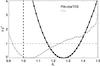 |
Fig. 1 Profile-likelihoods of the AL parameter reconstructed from the Plik high-ℓ likelihood alone (in grey) and when adding the lowTEB one (in black). The vertical dashed line recalls the expected ΛCDM value. |
Figure 1 also shows that the Plik-alone likelihood (in grey) gives  (4)which is compatible with 1.0. This difference from the Planck baseline result (Eq. (3)) seems to come from a tension between the low and high-ℓ likelihoods. Moreover, using a prior of the kind τ = 0.07 ± 0.02 (as in Like15) leads to AL = 1.16 ± 0.09, which goes in the same direction as Plik+lowTEB. This connection with τ will be discussed in the following section.
2.5. High- vs. low-ℓ likelihood results on τ and As
We further investigate the high vs. low-ℓ likelihood tensions from the point of view of two other parameters that are strongly correlated to AL: the reionization optical depth τ and the scalar perturbation amplitude As.
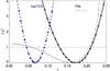 |
Fig. 2 High vs. low-ℓPlanck likelihood constraints on τ. The high-ℓ result is obtained with Plik (only) and is shown in black while the low-ℓ one is in dashed blue. Both are obtained within the ΛCDM model. The grey profile shows the result for Plik when AL is left free in the fits. |
Figure 2 shows, in black, the τ profile-likelihood reconstructed with Plik only, which gives  (5)This is higher than the maximum of the posterior reported in Like15 (Fig. 45) that is around 0.14 and is partly due to a volume effect (Sect. 2.3) and partly because of the class/camb difference highlighted in Appendix A. Using consistently class and the same methodology, our result is 2.2σ away from the τ determination with the lowTEB likelihood for which the profile-likelihood gives the same results as the MCMC marginalization (Like15):
  (6)represented as a blue line on Fig. 2.
Without fixing AL to 1 (grey curve on Fig. 2) the constraint on τ is much weaker, which illustrates the fact that the lensing of the CMB anisotropies in the high-ℓ likelihood is the main contributor to the τ measurement. Some constraining power still remains in particular for large τ values: this is due to the fact that the degeneracy between As and τ is broken for large τ when the reionisation bump at low ℓ enters the multipole range of Plik (ℓ> 30; Hu & White see 1997).
The discrepancy highlighted in Fig. 2 is directly related to the AL problem (Fig. 1), but is simpler to study. The high-ℓ likelihood requires a large τ value that is in tension with the low-ℓ-based result. In the AL test (Fig. 1) one combines both likelihoods.lowTEB pulls τ down. To match the spectra amplitude ( ), the high-ℓ likelihood pulls As down. Then AL, being fully anti-correlated to As (since
  ), shifts to adjust the lensed model to the data again.
Because of the 𝒜T degeneracy, the Plik-only estimate of As is also expected to be high. Indeed from a similar profile-likelihood analysis we obtain  (7)again discrepant by more than 2σ with the results from Plik+lowTEB, 3.089 ± 0.036 (PCP15).
In summary, the Plik high-ℓ likelihood alone converges to a consistent solution, AL ≃ 1, but with large τ and As values. Constraining τ down by adding the lowTEB likelihood (or a low prior) is compensated in the fits by increasing AL to match the data. To investigate the stability of those results, we will now use another Planck high-ℓ likelihoods.
3. The Hillipop likelihood
3.1. Description
Hillipop is one of the Planck high-ℓ likelihoods developed for the 2015 data release and is shorty described in Like15. Similarly to Plik, it is a Gaussian likelihood based on cross-spectra from the HFI 100, 143, and 217 GHz maps. The estimate of cross-spectra on data is performed using Xpol, a generalization of the Xspec algorithm (Tristram et al. 2005) to polarization. Figure 3 shows the combined TT spectrum with respect to the best-fit model that will be deepened later on.
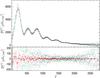 |
Fig. 3 Hillipop foreground-subtracted combined power-spectrum ( |
The differences with Plik were mentioned in Like15. The most significant are:
-
we use all the 15 half-mission cross-spectra built from the 100,143, and 217 GHz maps whilePlik uses only five of them;
-
we apply inter-calibration coefficients at the map level, resulting in five free parameters (one is fixed) while Plik uses two at the spectrum level;
-
we use point-sources masks that were obtained from a refined procedure that extracts Galactic compact structures;
-
as a result, our galactic dust component follows closely and is parametrized by the power law discussed in Planck Collaboration Int. XXX (2016);
-
we use foreground templates derived from Planck Collaboration XXX (2014) for the cosmic infrared background (CIB), and Planck Collaboration XXII (2016) for the SZ;
-
we use all multipole values (i.e., do not bin the spectra).
Using Hillipop leads to ΛCDM estimates that are very compatible with the other Planck ones but on As and τ (Like15, Sect. 4.2). Using a prior on τ of 0.07 ± 0.02, we obtain with Hillipopτ = 0.075 ± 0.019, while Plik gives a higher value τ = 0.085 ± 0.018 (Like15). Given the relation between τ and AL discussed in Sect. 2.5, we can therefore expect different results on AL.
Nuisance parameters for the Hillipop likelihood and Gaussian prior used during the likelihood maximization.
3.2. Results
The profile-likelihoods of AL derived from Hillipop with and without lowTEB is shown in Fig. 4. The Hillipop-alone profile is minimum near AL = 1.30 but is very broad : a 68% CL interval goes from .96 up to 1.42. We therefore conclude that Hillipop alone does not give a strict constraint on AL. In combination with lowTEB, using the same procedure as described in Sect. 2.4, we obtain  (8)This is slightly lower than the result obtained with Plik (Eq. (3)) but still discrepant with one by about 2σ.
Within the ΛCDM model, Fig. 5 compares Hillipop vs. lowTEB results on τ. The Hillipop profile on τ gives  (9)This is lower than the Plik result with similar error bars (Eq. (5)) and lies within 1.3σ of the low-ℓ measurement (Eq. (6)). In the ΛCDM+AL case, Hillipop only gives an upper limit. The difference with Plikτ profile (Fig. 2) is the sign of different correlations between AL and τ in these likelihoods.
One of the difference between the two likelihoods is in the definition of the foreground models. Moreover, with Planck data only, the accuracy on the foreground parameters is weak (especially for SZ and CIB amplitudes). In the next section, we will use the very-high-ℓ datasets. This both adds constraints on lensing through the high multipoles and better determines the foregrounds parameters and possibly modifies the non-trivial correlations between nuisance and cosmological parameters.
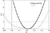 |
Fig. 4 Profile-likelihoods of the AL parameter reconstructed from the Hillipop likelihood alone (in grey) and when adding lowTEB (in black). The vertical dashed line recalls the expected ΛCDM value. |
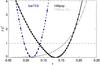 |
Fig. 5 Profile-likelihoods of the τ parameter using only the high-ℓHillipop likelihood: ΛCDM+AL free in the fits (in grey) and ΛCDM with fixed AL = 1 (in black). |
4. Adding very-high-ℓ data to constrain the foregrounds
4.1. Datasets
Atacama Cosmology Telescope.
We use the final ACT temperature power spectra presented in Das et al. (2014). These are 148 × 148, 148 × 218, and 218 × 218 power spectra built from observations performed on two different sky areas (south and equatorial) and during several seasons, for multipoles between 1000 and 10 000 (for 148 × 148), and 1500 to 10 000 otherwise.
South Pole Telescope.
We use two distinct datasets from SPT.
The higher ℓ part, dubbed SPT_high, uses results, described in Reichardt et al. (2012), from observations at 95, 150, and 220 GHz from the SPT-SZ survey. Their cross-spectra cover the ℓ range between 2000 and 10 000. These measurements were calibrated using WMAP 7yr data. A more recent analysis from the complete ~2500 deg2 area of the SPT-SZ survey is presented in George et al. (2015), dubbed SPT_high2014 hereafter. In this later release, cross spectra cover a somewhat broader ℓ range, between 2000 and 13 000. Both sets of cross spectra are however quite similar, but the later comes with a covariance matrix that includes calibration uncertainties. Its use makes our work harder since it was calibrated on the Planck 2013 data, which in turn had a calibration offset of 1% (at the map level) with respect to the Planck 2015 spectra. We thus prefer to use Reichardt et al. (2012) dataset as a baseline in our analyses, with free calibration parameters to match other datasets. We have checked that all results presented in this paper are stable when switching to George et al. (2015), in which case we have to set strict priors on recalibration parameters owing to the form of the associated covariance matrix.
We also include the Story et al. (2013) dataset, dubbed SPT_low, consisting of a 150 GHz power spectrum which ranges from ℓ = 650 to 3000. Some concerns were raised in Planck Collaboration XVI (2014) about the compatibility of this dataset with Planck data. The tension was actually traced to be with the WMAP+SPT cosmology and the Planck and SPT_low power spectra were found to be broadly consistent with each other (Planck Collaboration XVI 2014). As will be shown later, we do not see any sign of tension between the Planck 2015 data and the SPT_low dataset, nor any reason to exclude it.
4.2. Foregrounds modelling
For the very-high-ℓ astrophysical foregrounds, we chose to use a model as coherent as possible with what has been set-up for Hillipop, i.e., the same templates for tSZ, kSZ, CIB, and tSZ × CIB. Since they have been computed for the Planck frequencies and bandpasses, we have to extrapolate them to the ACT and SPT respective effective frequencies and bandpasses. For tSZ, we scale the template with the usual fν = xcothx/ 2−4 function (where x = hν/kBTCMB), using the effective frequencies for the SZ spectral distribution given in Dunkley et al. (2013). For CIB and tSZ × CIB, we start from templates in Jy2 sr-1 in the IRAS convention (νI(ν) = cste spectrum) for Planck effective frequencies and bandpasses. For CIB, we use the conversion factors from Planck to the ACT/SPT effective frequencies and bandpasses, assuming the Béthermin et al. (2012) SED for the CIB combined with unit conversion factors to KCMB, for the ACT and SPT bandpasses (Planck Collaboration IX 2014). These factors are given in Table 2.
Conversion factors used for the foreground template extrapolation to ACT and SPT bandpasses with the CIB SED.
For the tSZ × CIB component of the (ν1 × ν2) cross-spectrum (from the ACT or SPT dataset), we scale the nearest HFI cross-spectrum ( ) using the ratio
  (10)and then convert it to KCMB using the factors computed from the for the ACT and SPT bandpasses, as above. This scaling applies at the 15% level for the HFI cross-frequency templates, choosing the 143 × 143 one as a reference.
In addition, a few more specific templates have been added to each datasets:
-
Point sources: to mask resolved point sources, ACT and SPT usedtheir own settings to match each instrument’s sensitivity andangular resolution. The unresolved point source populationsin each case are thus different, so we introduce extra nuisanceparameters to model them. We model the unresolved point sourcecomponents in the ACT and SPT spectra with one amplitude
 parameter per cross-spectrum. Consequently, this introduces six nuisance parameters for the ACT, six for the SPT_high, and one for the SPT_low datasets, respectively (see Table 3).
 -
Galactic dust: following Dunkley et al. (2013) and Das et al. (2014), we model the dust contribution in the ACT power spectra as a power law
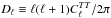
![Mathematical equation: \begin{equation} \mathcal{D}_{\ell}^{\rm dust}(i,j)\ =\ A_{\rm dust}^{\rm ACT}\left(\frac{\ell}{3000}\right)^{-0.7}\left(\frac{\nu_i\nu_j}{\nu_0^2}\right)^{3.8}\left[\frac{g(\nu_i)g(\nu_j)}{g(\nu_0)^2}\right]\cdot \end{equation}](/articles/aa/full_html/2017/01/aa27740-15/aa27740-15-eq104.png) (11)We therefore introduce two nuisance parameters, one for each part of the ACT dataset, and set the reference frequency ν0 at 150 GHz. For the SPT datasets, following Reichardt et al. (2012), we use a fixed template, with amplitudes 0.16, 0.21, and 2.19
(11)We therefore introduce two nuisance parameters, one for each part of the ACT dataset, and set the reference frequency ν0 at 150 GHz. For the SPT datasets, following Reichardt et al. (2012), we use a fixed template, with amplitudes 0.16, 0.21, and 2.19  at 95, 150, and 218 GHz, respectively and an ℓ-1.2 spatial dependency.
4.3. Likelihoods
We compute one likelihood for each of the five very-high-ℓ datasets following the method described in Dunkley et al. (2013). We use the respective published window functions to bin the (CMB + foregrounds) model, and the released covariance matrices to compute the likelihood. In all cases, these include beam uncertainties. Since we combine different datasets, we introduced nine additional nuisance parameters to account for their relative calibration uncertainties (at map level). Figure 6 shows a comparison of all the foreground-subtracted CMB spectra for the 150 × 150 component (which is almost common to all experiments), and Table 3 summarizes the characteristics of the datasets we use in the VHL likelihoods.
A detailed inspection of all cross-spectra per frequency and component has been performed and does not reveal any inconsistency with the Planck data. More details are given in Appendix C.
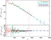 |
Fig. 6 Foreground-subtracted CMB cross-spectra of all the experiments used at ≃150 GHz. The solid line is the best fit of the Hillipop+VHL combination and is subtracted to obtain the bottom residual plot. The Hillipop likelihood uses individual multipoles up to 2000 and window functions have been accounted for in the very-high-ℓ data. |
Summary of the characteristics of the very-high-ℓ data used in this analysis.
4.4. First results and global consistency check
We first check that the combination of the ACT+SPT likelihoods (hereafter VHL) gives results consistent with Hillipop. We therefore sample the Hillipop and VHL likelihoods independently and compare their ΛCDM estimates in Fig. 7. Both datasets lead to similar cosmological parameters. However, an accurate measurement of Ωbh2 and Ωch2 requires a precise determination of the relative amplitudes of the CMB acoustic peaks for which the very-high-ℓ datasets are less sensitive. This is reflected by the width of the posteriors shown in Fig. 7.
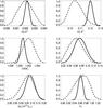 |
Fig. 7 Posterior distributions of the cosmological parameters obtained by sampling the Hillipop (soled line) and ACT+SPT (dashed) likelihoods independently. A prior of τ = 0.07 ± 0.02 is used in both cases. For clarity, we only show the cosmological parameters, but all nuisances are sampled. |
The χ2 contributions to the Hillipop+VHL+lowTEB best fit of each of the very-high-ℓ datasets are 58 /47(d.o.f.), 77 /90, and 651/710 for the SPT_low, SPT_high, and ACT datasets, respectively. None of these individual values indicate strong tension between the likelihood parts. We note that in all cases, the covariance matrices provided by the ACT and SPT groups, and used to compute the χ2, include non negligible, non-diagonal elements. For example, the visual impression from the SPT+low residuals, shown on Fig. C.3 is not excellent, but the χ2 from this part of the fit given above has a PTE of 13%, which is perfectly acceptable.
4.5. AL and τ results
As a second step, we perform the same analysis as in Sects. 2 and 3.2, adding the VHL likelihood to Hillipop and consider the AL profile-likelihood (with lowTEB) in Fig. 8. The result becomes  (12)now fully compatible with one.
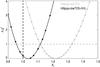 |
Fig. 8 Profile-likelihood for AL reconstructed from the Hillipop+lowTEB likelihood (in grey) and adding the very-high-ℓ ACT and SPT data (VHL) discussed in the text (in black). |
As seen in Sect. 5, the inclusion of the VHL data does not greatly change the cosmological parameters but, as expected, strongly constrains all the foregrounds including, through correlations, the ones specific to Planck data (dust and point source amplitudes). This is shown in Fig. 9.
We note that all Hillipop nuisance amplitudes (but the point sources) represent coefficients scaling foreground templates: it is remarkable that, after adding the VHL likelihood, they all lie reasonably (at least those for which we have the sensitivity) around one, which is a strong support in favor of the coherence of the foregrounds description.
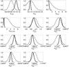 |
Fig. 9 Posterior distributions of the foreground Hillipop parameters with (solid line) and without (dashed line) the VHL likelihood. The definition of each parameter can be found in Table 1. |
For τ, combining the VHL with the Hillipop likelihood removes any sign of tension with lowTEB as shown in Fig. 10, and we obtain  (13)which is in excellent agreement with the lowTEB measurement (Eq. (6)).
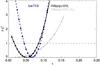 |
Fig. 10 Hillipop+VHL and lowTEB likelihood constraints on τ. The grey profile shows the result for Hillipop+VHL when AL is left free in the fits. The lowTEB one is in dashed blue. |
4.6. Robustness of the results
We tested a large number of configurations of the VHL dataset to establish whether the improvement comes from a particular one. Results are presented in Table 4.
It is difficult to draw firm conclusions from this exercise, since the number of extra nuisance parameters varyies in each case (see Table 3). The improvement on AL is most significant when combining several datasets, but also satisfactory as soon as one combines at least two of them. We note that all these results are highly correlated with each other, sinc they all make use of Hillipop. Even though central values very close to 1.0 may be preferable, it should be pointed out that there are several combinations that are compatible with 1.0 at the ~ 1σ level. This may indicate that the better the constraint on the high end of the power spectrum, the better the constraint on the AL control parameter (the lensing effect on  is not only a smearing of peaks and troughs but also a redistribution of power towards the high ℓ, above ~ 3000).
Since there is some overlap between SPT_low and SPT_high datasets, we expect some correlations between the SPT_low power-spectrum and, in particular, the 150 GHz spectrum of SPT_high. To check the impact on the results, we either removed the entire 150 GHz from SPT_high or the overlapping bins in multipole for each of the two datasets and re-ran the analysis. In all cases the results were similar with the combined one. For example, when removing the bins at ℓ< 3000 from the 150 × 150 GHz of SPT_high, we find AL = 0.99 ± 0.08, which is in good agreement with unity and with the results reported in Table 4. More checks are described in Appendix C.
Finally, we noticed that the SPT_high 220 × 220 spectrum lies slightly high with respect to the best fit (see Appendix C). Indeed, we get a better agreement in this case by increasing the contribution of the SPT dust amplitude. To check the impact on AL, we re-run the analysis, multiplying the dust level for all SPT spectra,  , by a factor of 3 and obtain
 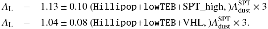 Compared with Table 4, the details of the SPT dust amplitude do not affect the final results.
Results on AL using Hillipop+lowTEB and various dataset combinations on the VHL side.
4.7. Where does the change on AL come from?
Adding the ACT and SPT data lowered the AL estimate. In this section, we try to pinpoint where the change came from.
As discussed in Sect. 2.1, Planck included the very-high-ℓ information in the Plik likelihood through a linear constraint between the thermal and kinetic components of the SZ foreground. When combining Hillipop with the VHL likelihood, a similar correlation is observed that in our units reads:  (14)To check whether this correlation is sufficient to capture the essentials of the very-high-ℓ information, we re-run the profile analysis adding to Hillipop+lowTEB only the prior in Eq. (14) and measure:
  (15)A comparison with Eq. (8) shows that, at least in our case, using this correlation does not capture the complexity of the full covariance matrix.
So, to check if the change came from a better constraint over all the foregrounds, we perform the following measurement: we use the Hillipop+lowTEB likelihood to determine AL as in Sect. 3.2 but fixing all the nuisance parameters to the best-fit value of Hillipop+lowTEB+VHL likelihood. A profile-likelihood analysis gives  compatible with unity at ~ 1σ as when using the very-high-ℓ data. We conclude that the shift for AL seems to come from the better determination of the foregrounds parameters. To determine which particular foreground parameters impacts the AL shift, we run an MCMC analysis sampling all the parameters (including AL) with the Hillipop+lowTEB and Hillipop+lowTEB+VHL likelihoods. The posterior distributions for AL and the foregrounds parameters in common between Hillipop and VHL are shown on Fig. 11.
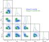 |
Fig. 11 Posterior distritions (68 and 95% levels) obtained from sampling the Hillipop+lowTEB and Hillipop+lowTEB+VHL likelihoods. We display the parameters most constrained by VHL. |
It is difficult to single out a particular correlation and we conclude that the improvement comes from the overall better constraint of the foregrounds.
5. Results on ΛCDM parameters
We have shown how the Hillipop likelihood is regularized by including the very-high-ℓ data. We have checked that it leads to results that are fully compatible with the lowTEB likelihood for τ and that their combination leads to an AL value that is now compatible with one. We then combine the three likelihoods and fix AL to one, to evaluate the impact on ΛCDM parameters. The comparison with the Planck published result is shown in Fig. 12. We note that:
-
Plik and Hillipop likelihoodsessentially share the same data;
-
the problem pointed out by AL is not a second-order effect: it directly affects Ωb, τ, and As results;
-
our regularized likelihood provides a lower σ8 estimate.
These results are obtained using only CMB data. To check the overall consistency and constrain the parameters, we also make use of some robust extra-information by including recent baryon acoustic oscillations (BAO) and supernovae (SN) results.
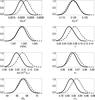 |
Fig. 12 Posterior distributions of the ΛCDM cosmological parameters obtained with our regularized likelihood (Hillipop+lowTEB+VHL, full line), compared to the Planck baseline result (Plik+lowTEB, dashed line). We recall that this former also includes some VHL information through an SZ correlation discussed in PCP15. The last row shows derived parameters. |
Estimates of cosmological parameters using MCMC techniques for the six ΛCDM parameters.
The BAO are generated by acoustic waves in the primordial fluid, and can be measured today through the study of the correlation functions of galaxy surveys. Owing to the fact that their measurement is sensitive to different systematic errors than the CMB, they help break the degeneracies, and are therefore further used in this paper to constrain the cosmological parameters. Here, we have used: the acoustic-scale distance ratio DV(z) /rdrag measurements6 from the 6dF Galaxy Survey at z = 0.1 (Beutler et al. 2014), and from BOSS-LowZ at z = 0.32. They have been combined with the BOSS-CMASS anisotropic measurements at z = 0.57, considering both the line of sight and the transverse direction, as described in Anderson et al. (2014).
Type Ia supernovae had a major role in the discovery of late time acceleration of the Universe and constitutes a powerful cosmological probe complementary to CMB constraints. We have used the JLA compilation (Betoule et al. 2014), which covers a wide redshift range (from 0.01 to 1.2).
Table 5 gives the results obtained with Hillipop+lowTEB (i.e., using only Planck data), then adding ACT+SPT likelihoods (i.e., only CMB) and finally also adding the BAO and SNIa likelihoods. Using only Planck data, the Hillipop+lowTEB results (first column in Table 5) are almost identical to the ones reported for “Planck TT +lowP” in PCP15, but for τ and As that are smaller, as explained in Sects. 3.2 and 2.5.
As discussed throughout this paper, adding the very-high-ℓ data (second column) releases the tension on the optical depth, leading to a value of τ around 0.06, as can be anticipated from Fig. 10. We also see a slight shift of Ωbh2 that is difficult to analyze since, at this level of precision, this parameter enters several areas of the Boltzmann computations (e.g., Hu & White 1997). Then, adding the BAO and SN data (third column) increases the precision on the parameters but does not change substantially their value.
We note that in all cases, σ8 is stable, e.g., Hillipop+lowTEB gives σ8 = 0.816 ± 0.015. This is only in mild tension with other astrophysical determinations such as weak lensing (Heymans et al. 2013) and Sunyaev-Zeldovich cluster number counts (Planck Collaboration XXIV 2016).
6. Conclusion
In this work, we have investigated the deviation of the AL parameter from unity and have found it to be of 2.6σ, using the Plik high-ℓ and lowTEB low-ℓPlanck likelihoods. For these demanding tests, we chose to consistently use the profile-likelihood method, which is well-suited to such studies. We first showed how this AL deviation is related to a difference in the τ estimations when performed using Plik or lowTEB alone.
The Hillipop likelihood has been built based on different foreground and nuisance parametrization. We have shown that Hillipop alone only very loosely constrains AL towards high values, and that its τ estimate lies closer to the low-ℓ measurement, albeit on the high-end side.
We then added to Hillipop, high angular resolution CMB data from the ground-based ACT and SPT experiments to further constrain the high-ℓ part of the CMB power spectrum and the foreground parameters. Cosmological parameters derived from this setup are shown to be more self-consistent, in particular the reconstructed τ value is coherent with the low-ℓ determination that was extracted from the lowTEB likelihood. They also pass the AL = 1.0 test.
We have shown that this regularization is quite robust against the details of the very-high-ℓ datasets used, and specific foreground hypotheses. We have also shown that it is not only related to a better determination of the foreground amplitudes but also seems to lie in their correlations.
The cosmological parameters determined from this combined CMB likelihood are also stable when adding BAO and SNIa likelihoods. This is, in particular, the case for σ8 that we always find close to 0.81. With respect to the cosmological parameters derived by the Planck Collaboration, the main differences concern τ and As, to which the former is directly correlated, and Ωbh2, which shifts by a fraction of σ. Other parameters are almost identical.
Improving on AL is a delicate task and it seems that the source of the regularization cannot be easily pinpointed. The choices of the Hillipop likelihood impact on the correlations between all the parameters, yielding a τ estimate in smaller tension with the low-ℓ likelihood. But this was not sufficient to relieve the AL tension. It is only by further constraining foregrounds using very-high-ℓ likelihoods that we were able to obtain a coherent picture over a broad range of multipoles.
One cannot exclude that the AL deviation from unity still partly results from an incomplete accounting of some residual systematics in the ACT, SPT, or Planck data.
During the review of this article, the Planck Collaboration released an estimate of the optical depth based on HFI cleaned maps (Planck Collaboration Int. XLVII 2016) and using the Lollipop likelihood (Mangilli et al. 2015). This new low-ℓ-only result, τ = 0.058 ± 0.012, increases the tension with the high-ℓ likelihoods to 2.6σ with Plik and 1.5σ with Hillipop and is fully compatible with our Hillipop+VHL combination (Eq. (13)).
Available in the Planck Legacy Archive (PLA): http://www.cosmos.esa.int/web/planck/pla
DV(z) is a function of the redshift (z) and can be expressed in terms of the angular diameter distance and the Hubble parameter, rdrag, is the comoving sound horizon at the end of the baryon drag epoch.
This single shot run last several minutes on 8 cores and requires about 30GB of memory.
Acknowledgments
We thank Guilaine Lagache for building and providing the point-source masks cleaned from Galactic compact structures, Marian Douspis for providing the SZ templates, and Marc Betoule for the development of the C version of the JLA likelihood.
References
- Anderson, L., Aubourg, É., Bailey, S., et al. 2014, MNRAS, 441, 24 [NASA ADS] [CrossRef] [Google Scholar]
- Béthermin, M., Daddi, E., Magdis, G., et al. 2012, ApJ, 757, L23 [NASA ADS] [CrossRef] [Google Scholar]
- Betoule, M., Kessler, R., Guy, J., et al. 2014, A&A, 568, A22 [NASA ADS] [CrossRef] [EDP Sciences] [Google Scholar]
- Beutler, F., Saito, S., Brownstein, J. R., et al. 2014, MNRAS, 444, 3501 [NASA ADS] [CrossRef] [Google Scholar]
- Blanchard, A., & Schneider, J. 1987, A&A, 184, 1 [NASA ADS] [Google Scholar]
- Blas, D., Lesgourgues, J., & Tram, T. 2011, J. Cosmol. Astropart. Phys., 7, 034 [Google Scholar]
- Calabrese, E., Slosar, A., Melchiorri, A., Smoot, G. F., & Zahn, O. 2008, Phys. Rev. D, 77, 123531 [NASA ADS] [CrossRef] [Google Scholar]
- Das, S., Louis, T., Nolta, M. R., et al. 2014, J. Cosmol. Astropart. Phys., 4, 14 [NASA ADS] [CrossRef] [Google Scholar]
- Di Valentino, E., Melchiorri, A., & Silk, J. 2016, Phys. Rev. D, 93, 023513 [NASA ADS] [CrossRef] [Google Scholar]
- Dunkley, J., Calabrese, E., Sievers, J., et al. 2013, J. Cosmol. Astropart. Phys., 7, 25 [Google Scholar]
- George, E. M., Reichardt, C. L., Aird, K. A., et al. 2015, ApJ, 799, 177 [NASA ADS] [CrossRef] [Google Scholar]
- Heymans, C., Grocutt, E., Heavens, A., et al. 2013, MNRAS, 432, 2433 [NASA ADS] [CrossRef] [Google Scholar]
- Hu, B., & Raveri, M. 2015, Phys. Rev. D, 91, 123515 [NASA ADS] [CrossRef] [Google Scholar]
- Hu, W., & White, M. 1997, ApJ, 479, 568 [NASA ADS] [CrossRef] [Google Scholar]
- James, F. 2007, Statistical Methods in Experimental Physics (World Scientific) [Google Scholar]
- Lesgourgues, J. 2011, ArXiv e-prints [arXiv:1104.2934] [Google Scholar]
- Lewis, A., & Challinor, A. 2006, Phys. Rep., 429, 1 [Google Scholar]
- Lewis, A., Challinor, A., & Lasenby, A. 2000, ApJ, 538, 473 [NASA ADS] [CrossRef] [Google Scholar]
- Mangilli, A., Plaszczynski, S., & Tristram, M. 2015, MNRAS, 453, 3174 [NASA ADS] [CrossRef] [Google Scholar]
- Planck Collaboration IX. 2014, A&A, 571, A9 [NASA ADS] [CrossRef] [EDP Sciences] [Google Scholar]
- Planck Collaboration XVI. 2014, A&A, 571, A16 [NASA ADS] [CrossRef] [EDP Sciences] [Google Scholar]
- Planck Collaboration XXX. 2014, A&A, 571, A30 [NASA ADS] [CrossRef] [EDP Sciences] [Google Scholar]
- Planck Collaboration I. 2016, A&A, 594, A1 [NASA ADS] [CrossRef] [EDP Sciences] [Google Scholar]
- Planck Collaboration VIII. 2016, A&A, 594, A8 [NASA ADS] [CrossRef] [EDP Sciences] [Google Scholar]
- Planck Collaboration XI. 2016, A&A, 594, A11 [NASA ADS] [CrossRef] [EDP Sciences] [Google Scholar]
- Planck Collaboration XIII. 2016, A&A, 594, A13 [NASA ADS] [CrossRef] [EDP Sciences] [Google Scholar]
- Planck Collaboration XXII. 2016, A&A, 594, A22 [NASA ADS] [CrossRef] [EDP Sciences] [Google Scholar]
- Planck Collaboration XXIV. 2016, A&A, 594, A24 [NASA ADS] [CrossRef] [EDP Sciences] [Google Scholar]
- Planck Collaboration Int. XVI. 2014, A&A, 566, A54 [NASA ADS] [CrossRef] [EDP Sciences] [Google Scholar]
- Planck Collaboration Int. XXX. 2016, A&A, 586, A133 [NASA ADS] [CrossRef] [EDP Sciences] [Google Scholar]
- Planck Collaboration Int. XLVII. 2016, A&A, 596, A108 [NASA ADS] [CrossRef] [EDP Sciences] [Google Scholar]
- Porter, F. 1996, Nucl. Instrum. Meth. Phys. Res. A, 368, 793 [Google Scholar]
- Reichardt, C. L., Shaw, L., Zahn, O., et al. 2012, ApJ, 755, 70 [NASA ADS] [CrossRef] [Google Scholar]
- Story, K. T., Reichardt, C. L., Hou, Z., et al. 2013, ApJ, 779, 86 [NASA ADS] [CrossRef] [Google Scholar]
- Tristram, M., Macías-Pérez, J. F., Renault, C., & Santos, D. 2005, MNRAS, 358, 833 [NASA ADS] [CrossRef] [Google Scholar]
Appendix A: Class vs. camb results
Our results were obtained using the classv2.3.2 Boltzmann code, which computes the temperature and polarization power spectra by evolving the cosmological background and perturbation equations. Besides being very clearly written in C and modular, class has a very complete set of precision parameters in a single place that enables us to study them efficiently. This makes it a perfect tool for developing modern high-precision cosmological projects.
We revisit the agreement between class and camb at the level required to estimate AL. For this purpose, we fix the cosmology to the Planck TT+lowP best fit and run class with three different settings:
-
the class default ones;
-
the high-quality (HQ) ones that are being used to obtain some smooth profile-likelihoods and are given in Table B.1;
-
the very high-quality (VHQ) ones corresponding to the maximal precision one can reasonably reach on a cluster7 and that are provided in class in the file cl_ref.pre.
For camb, we use the corresponding spectrum released in the Planck Legacy Archive. We compare the spectra on Fig. A.1 Generally speaking the agreement is at the (μK)2 level, which is below one percent agreement over the whole range. In practice, this means it does not impact on the ΛCDM parameters, as discussed in Like15.
The low-ℓ difference is not very important for data analysis since experiments are limited there by the cosmic variance. The asymptotic ≃1(μK)2 offset is more worrying and some ΛCDM extensions could be sensitive to this difference. Since the class spectrum is slightly lower than the camb one precisely in the high-ℓ region where AL has the largest impact, it should lead to a higher AL value. This is indeed observed and discussed in Sect. 2.4, but has a small effect on AL.
Finally we note that all class settings give similar results, in particular in their high-ℓ region, and that our HQ settings (used for profile-likelihoods) are smoother than the default ones and similar to the most extreme ones (VHQ).
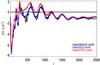 |
Fig. A.1 Difference of |
Appendix B: Optimization of profile-likelihoods
The computation of genuine profile-likelihoods requires exquisite minimization precision. Since the 68% confidence intervals are obtained by thresholding the profiles at 1, we need a precision on  , well below 0.1, which is challenging for a numerical method without analytic gradients. It has already been shown in Planck Collaboration Int. XVI (2014) how using the Minuit package and increasing the class precision parameters to high values (still keeping a reasonable computation time) enables us to achieve this goal.
High-precision settings of the class non-default parameters used in the profile-likelihood constructions.
Besides revisiting our high-precision parameters that are shown in Table B.1, we have improved our strategy further by using the following scheme:
-
1.
we use the picosoftware8 topre-compute a best fit solution. pico is based on the interpolationbetween spectra trained on the camb Boltzmannsolver. It is very fast and the minimization converges rapidlyowing to the smoothness between models;
-
2.
since camb computes only an approximation of the angular size of the sound horizon (θMC) while class computes it exactly (θs) we perform the change of variables by fixing the previous best-fit estimates and performing a 1D fit to θs only;
-
3.
we then have a good starting point to class and perform the minimization with a high-precision strategy (Migrad, strategy = 2 level);
-
4.
optionally: in some rare cases, the estimated minimum is not accurate enough (this can be identified by checking the profile-likelihood continuity). In this case, we use several random initialization points (typically 10) near the previous minimum, perform the same minimization, and keep the lowest
 solution.
In all cases we have checked that the pico results are similar to the final class ones but consider the latter to give more precise results since pico implements only an approximation to the AL parameter and was trained on an old camb version.
Appendix C: Very-high-ℓ consistency
Here we provide more details on the checks we performed to assess the ACT, SPT, and Planck spectra compatibility in the very-high-ℓ regime. Figures C.1–C.3 show the detailed fit of each component for each dataset. The components are obtained from the templates scaled according to the combined Hillipop+lowTEB+VHL fitted cosmological and nuisance parameters. The general agreement on the very-high-ℓ side is very good as shown by the χ2 for each dataset given in Sect. 4.4. We note that the points are largely correlated and that the exact χ2 computation involves the full covariance matrices provided by each experiment, which all contain non-negligible off-diagonal terms. For example, the χ2 from the SPT_low part is 58 for 47 deg of freedom, which has a 13% PTE. Some small excess in data seems to show up in the SPT_high 220 × 220 GHz spectrum above ℓ = 3000. In Sect. 4.6 we checked that this does not influence any of our results.
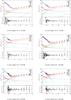 |
Fig. C.1 Power spectra of CMB and foregrounds as fitted by the Hillipop+VHL likelihood, compared with ACT data. The use of window functions explain why the CMB component sometimes reappears at the very end of the multipole range. |
 |
Fig. C.2 Power spectra of CMB and foregrounds as fitted by the Hillipop+VHL likelihood compared with SPT_high data. |
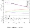 |
Fig. C.3 Power spectra of CMB and foregrounds as fitted by the Hillipop+VHL likelihood compared with SPT_low data. |
To check that the overlap in the data used on the SPT_lowand SPT_high datasets, we did three additional profile likelihood analyses for AL. First, we ignored the 150 GHz data from SPT_high, recomputing accordingly the inverse covariance matrix used in the χ2 computation. We also tested the impact of removing in the SPT_low spectrum all bins above ℓ = 3000 (which are accounted for in the SPT_high part. To do this, we again recomputed the inverse covariance matrix. Finally, we omit in the SPT_high part bins at 150 GHz at ℓ< 3000. These results are reported in Table C.1. All are compatible with each other and with unity.
Results on AL using Hillipop+lowTEB and VHL, making various attempts at removing the correlated part between SPT_high and SPT_low: (a) w/o 150 GHz data; (b) w/o overlapping bins; (c)w/o overlapping bins.
All Tables
Nuisance parameters for the Hillipop likelihood and Gaussian prior used during the likelihood maximization.
Conversion factors used for the foreground template extrapolation to ACT and SPT bandpasses with the CIB SED.
Results on AL using Hillipop+lowTEB and various dataset combinations on the VHL side.
Estimates of cosmological parameters using MCMC techniques for the six ΛCDM parameters.
High-precision settings of the class non-default parameters used in the profile-likelihood constructions.
Results on AL using Hillipop+lowTEB and VHL, making various attempts at removing the correlated part between SPT_high and SPT_low: (a) w/o 150 GHz data; (b) w/o overlapping bins; (c)w/o overlapping bins.
All Figures
|
Fig. 1 Profile-likelihoods of the AL parameter reconstructed from the Plik high-ℓ likelihood alone (in grey) and when adding the lowTEB one (in black). The vertical dashed line recalls the expected ΛCDM value. |
| In the text | |
|
Fig. 2 High vs. low-ℓPlanck likelihood constraints on τ. The high-ℓ result is obtained with Plik (only) and is shown in black while the low-ℓ one is in dashed blue. Both are obtained within the ΛCDM model. The grey profile shows the result for Plik when AL is left free in the fits. |
| In the text | |
|
Fig. 3 Hillipop foreground-subtracted combined power-spectrum ( |
| In the text | |
|
Fig. 4 Profile-likelihoods of the AL parameter reconstructed from the Hillipop likelihood alone (in grey) and when adding lowTEB (in black). The vertical dashed line recalls the expected ΛCDM value. |
| In the text | |
|
Fig. 5 Profile-likelihoods of the τ parameter using only the high-ℓHillipop likelihood: ΛCDM+AL free in the fits (in grey) and ΛCDM with fixed AL = 1 (in black). |
| In the text | |
|
Fig. 6 Foreground-subtracted CMB cross-spectra of all the experiments used at ≃150 GHz. The solid line is the best fit of the Hillipop+VHL combination and is subtracted to obtain the bottom residual plot. The Hillipop likelihood uses individual multipoles up to 2000 and window functions have been accounted for in the very-high-ℓ data. |
| In the text | |
|
Fig. 7 Posterior distributions of the cosmological parameters obtained by sampling the Hillipop (soled line) and ACT+SPT (dashed) likelihoods independently. A prior of τ = 0.07 ± 0.02 is used in both cases. For clarity, we only show the cosmological parameters, but all nuisances are sampled. |
| In the text | |
|
Fig. 8 Profile-likelihood for AL reconstructed from the Hillipop+lowTEB likelihood (in grey) and adding the very-high-ℓ ACT and SPT data (VHL) discussed in the text (in black). |
| In the text | |
|
Fig. 9 Posterior distributions of the foreground Hillipop parameters with (solid line) and without (dashed line) the VHL likelihood. The definition of each parameter can be found in Table 1. |
| In the text | |
|
Fig. 10 Hillipop+VHL and lowTEB likelihood constraints on τ. The grey profile shows the result for Hillipop+VHL when AL is left free in the fits. The lowTEB one is in dashed blue. |
| In the text | |
|
Fig. 11 Posterior distritions (68 and 95% levels) obtained from sampling the Hillipop+lowTEB and Hillipop+lowTEB+VHL likelihoods. We display the parameters most constrained by VHL. |
| In the text | |
|
Fig. 12 Posterior distributions of the ΛCDM cosmological parameters obtained with our regularized likelihood (Hillipop+lowTEB+VHL, full line), compared to the Planck baseline result (Plik+lowTEB, dashed line). We recall that this former also includes some VHL information through an SZ correlation discussed in PCP15. The last row shows derived parameters. |
| In the text | |
|
Fig. A.1 Difference of |
| In the text | |
|
Fig. C.1 Power spectra of CMB and foregrounds as fitted by the Hillipop+VHL likelihood, compared with ACT data. The use of window functions explain why the CMB component sometimes reappears at the very end of the multipole range. |
| In the text | |
|
Fig. C.2 Power spectra of CMB and foregrounds as fitted by the Hillipop+VHL likelihood compared with SPT_high data. |
| In the text | |
|
Fig. C.3 Power spectra of CMB and foregrounds as fitted by the Hillipop+VHL likelihood compared with SPT_low data. |
| In the text | |
Current usage metrics show cumulative count of Article Views (full-text article views including HTML views, PDF and ePub downloads, according to the available data) and Abstracts Views on Vision4Press platform.
Data correspond to usage on the plateform after 2015. The current usage metrics is available 48-96 hours after online publication and is updated daily on week days.
Initial download of the metrics may take a while.