| Issue |
A&A
Volume 596, December 2016
|
|
|---|---|---|
| Article Number | A60 | |
| Number of page(s) | 20 | |
| Section | Catalogs and data | |
| DOI | https://doi.org/10.1051/0004-6361/201628189 | |
| Published online | 30 November 2016 | |
NIBLES – an HI census of stellar mass selected SDSS galaxies
II. Arecibo follow-up HI observations⋆
1 University of Massachusetts, Astronomy Program, LGRT-B 619E, Amherst, MA 01003, USA
e-mail: This email address is being protected from spambots. You need JavaScript enabled to view it.
2 GEPI, Observatoire de Paris, CNRS, Université Paris Diderot, 5 place Jules Janssen, 92190 Meudon, France
3 Station de Radioastronomie de Nançay, Observatoire de Paris, CNRS/INSU USR 704, Université d’Orléans OSUC, route de Souesmes, 18330 Nançay, France
4 Institut d’Astrophysique de Paris, UMR 7095, CNRS, Université Pierre et Marie Curie, 98bis boulevard Arago, 75014 Paris, France
5 Arecibo Observatory, National Astronomy and Ionosphere Center, Arecibo, PR 00612, USA
Received: 25 January 2016
Accepted: 10 July 2016
Abstract
We obtained Arecibo Hi line follow-up observations of 154 of the 2600 galaxies in the Nançay Interstellar Baryons Legacy Extragalactic Survey (NIBLES) sample. These observations are on average four times more sensitive than the original observations at the Nançay Radio Telescope. The main goal of this survey is to characterize the underlying Hi properties of the NIBLES galaxies which were undetected or marginally detected at Nançay. Of the Nançay non-detections, 85% were either clearly or marginally detected at Arecibo, while 89% of the Nançay marginal detections were clearly detected. Based on the statistics of the detections relative to g−i color and r-band luminosity (Lr) distribution among our Arecibo observations, we anticipate ~60% of our 867 Nançay non-detections and marginal detections could be detected at the sensitivity of our Arecibo observations. Follow-up observations of our low luminosity (Lr < 108.5L⊙) blue sources indicate that they have, on average, more concentrated stellar mass distributions than the Nançay detections in the same luminosity range, suggesting we may be probing galaxies with intrinsically different properties. These follow-up observations enable us to probe Hi mass fractions, log(MHI/M⋆) 0.5 dex and 1 dex lower, on average, than the NIBLES and ALFALFA surveys respectively.
Key words: surveys / galaxies: general / galaxies: distances and redshifts / radio lines: galaxies / galaxies: ISM
Reduced spectra are only available at the CDS via anonymous ftp to cdsarc.u-strasbg.fr (130.79.128.5) or via http://cdsarc.u-strasbg.fr/viz-bin/qcat?J/A+A/596/A60
© ESO, 2016
1. Introduction
The optical luminosity function (LF) and the Hi mass function (HIMF) are two of the most important and fundamental tracers of the volume density distribution of galaxies in the universe. They yield clues to both the baryonic and dark matter content of galaxies, as well as their evolutionary histories. Consequently, there are many applications for which the LF and HIMF can be used, for example, as constraints in galaxy formation models (see, e.g., Benson et al. 2003; Lu et al. 2014).
Many studies have attempted to constrain both of these functions over the years. Since the LF was first fitted to an analytic form by Schechter (1976), many subsequent studies have attempted to analyze its various properties and constrain its parameters (see, e.g., Felten 1985; Efstathiou et al. 1988; Loveday et al. 1992, 2015; Blanton & Collaboration 2001; Blanton et al. 2003; Montero-Dorta & Prada 2009; McNaught-Roberts et al. 2014). The HIMF, having the same functional form as the LF, has also been analyzed in detail, although to a somewhat lesser extent (see, e.g., Zwaan et al. 1997, 2003; Kilborn et al. 1999; Kovac et al. 2005; Springob et al. 2005; Martin et al. 2010; Hoppmann et al. 2015).
To date, both these functions have been treated separately in their analyses. One of the main goals of the Nançay Interstellar Baryons Legacy Extragalactic Survey (NIBLES) is to study the inter-relation between these two fundamental population tracers. More specifically, we want to analyze the HIMF and other galaxy properties as a function of optical luminosity. To achieve this goal, we carried out a 21 cm Hi line survey at the 100 m class Nançay Radio Telescope (NRT). The final observed sample consists of 2600 galaxies selected from the Sloan Digital Sky Survey (SDSS; see, e.g., York et al. 2000) with radial velocities 900 <cz< 12 000 km s-1. The galaxies were selected to be distributed evenly over their entire range of absolute z-band magnitudes (~− 13.5 to − 24), which was used as a proxy for total stellar mass – see van Driel et al. (2016, Paper I) for further details.
The NIBLES galaxy selection criteria are:
-
1.
must have both SDSS magnitudes and opticalspectrum;
-
2.
must lie within the local volume (900 <cz< 12 000 km s-1);
-
3.
uniform sampling of each 0.5 mag wide bin in absolute z-band magnitude, Mz;
-
4.
preferentially observe nearby objects;
-
5.
no a priori selection on color.
NIBLES, with its relatively uniform selection of galaxies that are based on total stellar mass, is aimed to complement other recent and/or ongoing large Hi surveys in the local volume, in particular, blind surveys such as ALFALFA (e.g., Haynes et al. 2011). One main advantage of NIBLES over blind Hi surveys is our increased on-source integration time, which enables us to reduce the rms noise of the observations. Each NIBLES source was initially observed at Nançay for about 40 min of telescope time, resulting in a mean rms noise of ~3 mJy at 18 km s-1 resolution. In the case of weak or non-detections, observations were repeated (as time allowed) resulting in a target rms noise between 1.5 and 1.8 mJy for the majority of our undetected sample. However, there were a number of sources where follow-up time was unavailable to achieve the desired rms, which resulted in a mean of 2.3 mJy for the remainder of the undetected sample, yielding a bimodal rms noise distribution (see Paper I).
Of the 2600 NIBLES galaxies, 1733 (67%) were clearly detected, 174 (7%) marginally detected, and 693 (27%) were not detected. To adequately quantify our Hi distribution across the optical LF, we need to gain a statistical understanding of the underlying Hi distribution of sources which were undetected at Nançay. We therefore carried out pointed observations of 90 undetected or marginally detected galaxies at the 305 m Arecibo radio telescope, which gives us a noise level reduction by about a factor of four. Additionally, we had a number of sources suffering from observational problems at Nançay which we re-observed at Arecibo, and during periods of time when primary target sources were unavailable, we observed detected NIBLES sources to compare flux calibrations at the two observatories. In total, we observed 154 galaxies from the NIBLES sample (see Sect. 2 and Paper I for details).
Here we present the results from these follow-up observations along with a brief synopsis of the differences in the data between the Nançay and Arecibo samples. The main purpose of this paper is data presentation. Further analysis will be carried out in subsequent papers. In Sect. 2 we describe the selection of the observed sample of galaxies and in Sect. 3, the observations and data reduction. The results are presented in Sect. 4 and discussed in Sect. 5 We present our conclusions in Sect. 6. An analysis of this data regarding the impact on our Hi distribution as a function of optical luminosity will be presented in Paper III (Butcher et al., in prep.). All source numbers presented in this paper refer to the NIBLES source number, which can be cross-referenced with other common source names in the tables presented here and in Paper I.
2. Sample selection
Our total sample of Arecibo follow-up galaxies consists of 154 sources. Of these, 90 are classified as either non-detections or marginal detections at Nançay, with the remaining 64 consisting of sources initially suffering from observational problems such as OFF beam detections or RFI and a handful of sources used for flux comparison between the two telescopes. Of these 64, ten were excluded from the original NIBLES catalog because their Nançay observations contained technical problems which we were not able to overcome (listed in Table 5).
Of the 90 Nançay non-detected or marginally detected galaxies, 59 were selected based on color (u−z < 2) and radial velocity (cz < 4000 km s-1) for the specific reason that these blue, nearby galaxies would normally be expected to have Hi and yet were undetected at Nançay.
3. Observations and data reduction
The Arecibo radio telescope uses a 305 m diameter spherical primary mirror and covers a declination range of − 1° < δ < 38° with pointing accuracy of about 5′′. We used the L-band wideband receiver (L-wide) with the Wideband Arecibo Pulsar Processor (WAPP) correlator backend using two polarizations with a bandpass of 50 MHz (approximately 10 600 km s-1) across 4096 frequency channels corresponding to a channel separation of 2.6 km s-1 at z ~ 0. The L-wide receiver has a half power beam width of approximately 3′.5 and yields an effective system temperature typically between 28 and 32 K. Data were taken in standard 5/5 min integration ON/OFF position switching mode. All galaxies were observed for a minimum of one 5/5 min cycle, and some of the blue low-luminosity galaxies were observed longer depending on telescope time and signal strength after the first observation.
Throughout this paper, all radial velocities given are heliocentric, and all Hi-line related parameters are according to the conventional optical definition (V = c(λ – λ0)/λ0).
Observations were carried out in two sessions, between December 2008 and October 2009 and between March and September 2012 for a total of 59 h.
Data were reduced using a combination of Phil Perillat’s IDL routines and Robert Minchin’s CORMEASURE routine from the Arecibo Observatory. All Hi spectra were Hanning smoothed to a median velocity resolution of 18.7 km s-1 to match the 18 km s-1 resolution of the NRT spectra as closely as possible. All Hi spectra shown here have a heliocentric, optical (cz) radial velocity scale.
Two of our sources, 1260 and 2434 (i.e., PGC 4546173 and CGCG 427-032), suffered from a baseline ripple with a wavelength corresponding to approximately 210 km s-1 which we were able to remove via a Fourier transform, see Appendix A for details.
4. Results
The Arecibo observations enabled us to probe our sample about four times deeper on average than at Nançay. The mean rms noise of the Nançay undetected sample is 2.33 mJy whereas the mean rms noise of our Arecibo observations is 0.57 mJy, both at 18 km s-1 resolution.
As with our Nançay data, we divided the sources into detected, marginally detected, and non-detected categories. This was accomplished through visual inspection of each Hi spectrum by three independent adjudicators (ZB, WvD, SES). Disagreements were discussed until a consensus was reached. The galaxies in the marginal detection category have Hi line spectra with a peak signal-to-noise ratio less than four, but coinciding with the SDSS optical velocity. The galaxies in this category would most likely be missed in a survey of objects with previously unknown velocity. However, the low probability of a strong noise peak coinciding with the SDSS optical velocity lends greater credibility to the likelihood that these peaks represent real signals.
There is generally very good agreement (<3 km s-1 on average) between the DR9 heliocentric velocities and our Hi velocities, with the exception of three cases. These three outliers, sources 1631, 2434, and 2606 (i.e., NGC 4290, CGCG 427-032, and NGC 3772 respectively) all have velocity discrepancies larger than 50 km s-1. Source 1631 has the SDSS spectral fiber positioned out in its disk, blueshifting the overall redshift measurement. Source 2434 is confused with a secondary source in the Arecibo beam, but source 2606 suffers no obvious signs of confusion or spectral fiber offsets and the optical spectrum does not appear noisy (see Fig. B.1). However, source 2606 is also listed in de Vaucouleurs et al. (1991) as having a heliocentric velocity of 3478 ± 50 km s-1 which agrees with our Hi velocity of 3423 ± 7 km s-1.
The optical data listed are in general from the SDSS DR9 (see also Paper I) with the median total stellar masses and star-formation rates taken from the corresponding publicly available SDSS added-value MPA-JHU catalogs (Brinchmann et al. 2004; Kauffmann et al. 2003; Salim et al. 2007; Tremonti et al. 2004) where available. In cases where estimates are not available, stellar masses, specific star formation rates (sSFR), and gas mass fractions (log(MHI/M⋆)) are marked as “—”.
Due to the limited redshift range of NIBLES, the difference in luminosity distances used for our Hi masses and the stellar mass estimates from MPA-JHU are less than a few percent in the most extreme cases. This systematic difference is far less than the typical uncertainty in the stellar mass estimates themselves, which are on the order of 20%.
Listed throughout the tables are the following properties of the target galaxies:
-
RA and Dec: Right Ascension and Declination in J2000.0coordinates, as used for the observations;
-
other name: common catalog name, other than the SDSS;
-
Vopt: heliocentric radial velocity (cz) measured in the optical (in km s-1), from Paper I;
-
log(M⋆): total median stellar mass estimates (in M⊙);
-
log(sSFR): specific star formation rate, or SFR/M⋆ (in yr-1);
-
g−z: g−z integrated color of the galaxy using SDSS model magnitudes, corrected for Galactic extinction, following Schlegel et al. (1998; in mag);
-
Mg: integrated absolute g-band model magnitude, corrected for Galactic extinction following Schlegel et al. (1998);
-
rms: rms noise level values of the Hi spectra (in mJy);
-
VHI: heliocentric radial velocity (cz) of the center of the Hi line profile (in km s-1);
-
W50, W20: velocity widths measured at 50% and 20% of the Hi profile peak level, respectively, uncorrected for galaxy inclination (in km s-1);
-
FHI: integrated Hi line flux (in Jy km s-1);
-
SNR: peak signal-to-noise ratio, which we define as the peak flux density divided by the rms; For non-detections, the SNR listed is the maximum found in the expected velocity range of the Hi profile;
-
S/N: signal-to-noise ratio determined taking into account the line width, following the ALFALFA Hi survey formulation from Saintonge (2007): S/N = 1000(FHI/W50) (W50/2 R)0.5)/rms, where R is the velocity resolution, 18.7 km s-1 on average;
-
log(MHI): total Hi mass (in M⊙), where MHI = 2.36·105·D2.FHI, where D = V/70 is the galaxy’s distance (in Mpc). In the cases of non-detections, 3σ upper limits are listed for a flat-topped profile with a width depending on the target’s r-band luminosity, Lr, according to the upper envelope in the W20 – Lr relationship of our Nançay clear, non-confused detections (see Paper I);
-
log(MHI/M⋆): ratio of the total Hi and stellar masses.
Estimated uncertainties are given after the values in the tables. Uncertainties in the central Hi line velocity, VHI, and in the integrated Hi line flux, FHI, were determined following Schneider et al. (1986, 1990) as, respectively
 where R is the instrumental resolution, 18.7 km s-1, SNR is the peak signal-to-noise ratio of a spectrum and rms is the root mean square noise level (in Jy). Following Schneider et al., the uncertainty in the W50 and W20 line widths is expected to be 2 and 3.1 times the uncertainty in VHI, respectively.
Table 1 lists all 72 sources detected at Arecibo which were either undetected (55 sources) or marginally detected (17 sources) at Nançay. Table 2 lists the five Arecibo marginal detections which were undetected at Nançay, and Table 3 lists the 15 sources not detected at Arecibo, including 11 Nançay non-detections, two Nançay marginal detections and two others flagged as NRT confused detections which were not detected at Arecibo due to its smaller beam size.
In Table 4 we compare line flux parameters of galaxies we detected at both Arecibo and Nançay and in Table 5 we list the ten sources detected at Arecibo which were not included in our final Nançay sample due to data problems (see Paper I).
Basic optical and Hi data – Arecibo detections of Nançay non-detections and marginals.
Basic optical and Hi data – Arecibo marginal detections of Nançay non-detections.
The following types of cases have been flagged in the tables following the naming conventions in Paper I:
-
C (3 cases): Hi detection of the target galaxyconfused by another galaxy within the Arecibo telescope beam;
-
C3 (1 case): Hi detection of the target galaxy confused by another galaxy in the Arecibo telescope beam, but the secondary source likely contributes a minor amount of flux to the total observed flux;
-
K (8 cases): Nançay Hi detection either clearly or possibly confused by another galaxy within the NRT beam;
-
D (2 cases): baseline ripple removed from Hi spectrum (see Sect. 3);
-
M (19 cases): original Nançay detection classification changed to marginally detected;
-
R (2 cases): sources possibly resolved by the Arecibo beam. These sources have an SDSS optical image with a diameter about the same size as the Arecibo beam which is expected to lead to an underestimate of their total Hi flux.
Color SDSS images alongside the Hi line spectra of our Arecibo detections are shown in Fig. B.1, marginal detections are presented in Fig. B.2, and non-detections in Fig. B.3.
Due to the updated detection category classifications and reprocessing of the Nançay data, our Arecibo follow-up sample now consists of 54 galaxies detected at Nançay (of which 52 were detected at Arecibo and the remaining two are confused detections at Nançay where the signal is from a secondary source) as well as 90 galaxies which are either undetected (71) or marginally detected (19) at Nançay and ten galaxies for which we have no useable Nançay data. These ten have been added to the NIBLES catalog and assigned succeeding source numbers, see Table 5.
4.1. Flux comparison between Arecibo and Nançay
For our ten calibration sources which have a Nançay peak signal-to-noise ratio greater than 8, we compared the Hi line flux ratios at both telescopes using a weighted mean. Each source was weighted by the inverse square of its flux uncertainty to more heavily weight the sources with lower errors. The resulting Arecibo/NRT flux ratio is 1.19 ± 0.08 where the uncertainty is given by the standard deviation of the weighted mean. This offset is consistent with the flux offset discussed in Paper I, however detailed analysis of this flux scale difference is beyond the scope of this paper (see Paper I for details).
5. Discussion
5.1. Arecibo detection rate of Nançay non-detections and marginal detections
In this section and the remainder of this paper we focus on the Arecibo follow-up sample consisting of the 90 galaxies observed at Arecibo which were either undetected or marginally detected at Nançay. The Nançay marginal detections are included with the Nançay non-detections for the analyses presented below since the marginal detection category had not yet been implemented at the time of this our Arecibo survey.
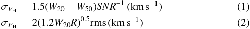
Of our 90 Nançay non-detections or marginal detections, 72 had sufficient Hi line flux to be clearly detected at Arecibo, resulting in a high overall detection rate of 80% (greater than 85% counting Arecibo marginal detections). One likely reason for this high detection rate is that most of our sample consisted of predominately blue, nearby star-forming galaxies. This color bias is obvious in Fig. 1, which shows the number of galaxies observed and detected as a function of g−i color. All of the galaxies with g−i colors bluer than 0.3 were detected, whereas only one third of the reddest galaxies were detected.
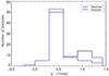 |
Fig. 1 Number of galaxies as a function of g−i color, corrected for Galactic extinction following Schlegel et al. (1998). The black line is the total number of observed galaxies in each 0.25 mag wide bin and the blue line the total number of detected galaxies. The peak around 0.5 mag is due to our specific selection of blue objects (see Sect. 2). |
A color−magnitude diagram of integrated g−i colors as a function of r-band luminosity is shown in Fig. 2 for our detections, non-detections, and marginals of both the Arecibo and the Nançay samples. The dichotomy in both color and luminosity between Hi detections and non-detections is obvious in this plot. At the low luminosity end (log(Lr) < 9), the Nançay data show a color dichotomy with the detections clustering around g−i ~ 0.4 (commonly referred to as the “blue cloud”) and non-detections clustering around g−i ~ 0.8 (commonly referred to as the “red sequence”). This dichotomy has not previously been seen in larger surveys such as Gavazzi et al. (2010) or Huang et al. (2012), primarily due to the smaller dynamic range probed by the former and by the exclusion of lower luminosity red galaxies in the latter. However, due to the NIBLES selection criteria and our ~1 dex larger dynamic range, our sample contains a clear separation by color at low luminosities.
The sole Arecibo non-detection in this low-luminosity range (inverted blue triangle in Fig. 2) has a relatively red color, but several other low-luminosity red sources were detected, and two of the bluer low-luminosity galaxies were only marginally detected at Arecibo. Further follow-up of these red, low luminosity sources is needed to establish the Hi mass properties of this low-luminosity red population.
The blue cloud largely disappears at luminosities higher than log(Lr) = 9.5, where the majority of sources cluster around g−i color of ~1.2. However, aside from the fact that these galaxies have relatively more non-detections compared to the low luminosity galaxies, the mixture of detections with non-detections suggests that a not insignificant fraction of the red sequence galaxies may contain detectable levels of Hi. However, deeper follow-up observations of red sequence galaxies will be needed to answer this question.
Basic optical and Hi data – Arecibo non-detections.
Basic optical and Hi data – comparison of Arecibo and Nançay detections.
 |
Fig. 2 Integrated g−i color, in mag, as function of absolute r-band luminosity, log(Lr) in L⊙, both corrected for Galactic extinction following Schlegel et al. (1998). Nançay detections, marginals, and non-detections are represented by gray dots, open gray circles, and open red circles respectively. Arecibo detections, marginals, and non-detections are respectively represented by black solid stars, open stars, and blue downward triangles. The low luminosity end (log(Lr) <9) shows a color dichotomy with Hi detections and non-detections clustering around g−i ~ 0.4 and g−i ~ 0.8 respectively, showing a clear distinction between the blue cloud and red sequence galaxies. Above luminosities of log(Lr) ~ 9.5, the blue cloud disappears while the red sequence galaxies shift to redder colors, g−i ~ 1.2. |
We compare the detection fractions as a function of g−i color and Lr for our Nançay and Arecibo samples in Fig. 3, counting the marginal detections in with the non-detections. The Nançay data show a global decrease in detection fraction as a function of color while the Arecibo data show a rather sharp drop by about a factor of 2.5 above g−i ~ 0.8. As a function of luminosity, the Nançay detection percentage shows no decrease below log(Lr) ~ 10 while the Arecibo sample shows a two times lower detection rate above log(Lr) ~9. The plotted uncertainties in the Nançay data points are the standard deviation of the binomial distribution, given by  (3)where P is the probability of detection, given by m/n where m is the number of detections and n is the total number in a particular bin. The Arecibo data generally have a small number of sources per bin which in some cases makes the uncertainty difficult to quantify. We therefore adopted the 90% confidence limits from Gehrels (1986) for dealing with the small number statistics of the Arecibo sample.
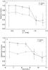 |
Fig. 3 a) Detection fraction for the NIBLES Nançay sample (gray) and the Arecibo follow-up sample (black) as a function of g−i color. b) Detection fractions as a function of r-band luminosity. Error bars for the Nançay data are the standard deviation of the binomial distribution and the error bars for the Arecibo data were calculated following Gehrels (1986) using the 90% confidence intervals. Bin sizes are 0.3 for a) and 1 for b). |
If we apply the Arecibo detection percentages to the Nançay sample, we would expect (with observations of the same sensitivity as our Arecibo sample, i.e., four times lower noise than at Nançay) to detect about 60% (or ~530) of the 867 Nançay non-detections and marginal detections: based on color statistics the expected number is, 526 ± 160 and it is 546 ± 158 from the luminosity data (see Fig. 4). The uncertainty is calculated by adding in quadrature the fractional uncertainty in each g−i or Lr bin, respectively.
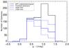 |
Fig. 4 Total number of galaxies either undetected or marginally detected at Nançay that would be detectable with the same sensitivity as our Arecibo observations, as a function of g−i color. Black indicates Nançay non-detections and marginals, whereas the solid blue line is the estimated number of galaxies that would be detectable based on our Arecibo sample detection rate. The blue dashed and dash-dotted lines are based on, respectively, the upper and lower envelopes of the uncertainties in the detection rate, see Fig. 3. |
We have a total remaining sample of 442 Nançay undetected or marginally detected galaxies within the Arecibo declination range, consisting mostly of redder low-luminosity (below Lr~109L⊙) sources as well as some higher luminosity red sequence galaxies. Based on our current results, we estimate that comparable observations of the remaining 442 sources at Arecibo would require about 160 h of telescope time: 60% to be observed for our standard 5 min on-source integrations and the other 40% for 15 min each. If detection statistics follow the same pattern as this sample, we would expect about 60% of the remaining Nançay undetected sample to be detected at Arecibo. This would bring the over-all detection rate of the NIBLES sample within the Arecibo declination range to ~89%, and the global detection rate to ~77%. If we extrapolate these detection percentages to the entirety of the NIBLES sample, we would expect the NIBLES global detection rate to increase to ~86%.
Of the subset of our sample that was selected on low luminosity and blue color, we achieved a 100% detection rate (including the Arecibo marginal detections). We also managed to detect several red sequence galaxies with very low Hi stellar mass ratios, log(MHI/M⋆) <− 2 (see Fig. 9). Two of these have stellar masses greater than 1011.5M⊙, placing them in an area of MHI/M⋆–M⋆ parameter space not probed by the ALFALFA survey and as yet virtually unexplored.
5.2. Physical properties of Arecibo-detected galaxies
In Paper I we used the W20−Lr relationship to estimate the maximum Hi line width a galaxy typically has for a given luminosity. The least-squares fit to this relationship is log(W20) = 0.4 + 0.2·log (Lr). When comparing the Arecibo data to the Nançay data, the Arecibo detections appear to have W20 values that are about 35% narrower than the corresponding Nançay detections of the same luminosity. This is due in large part to our selection of low luminosity blue dwarf galaxies, which are predominately supported by velocity dispersion rather than rotation. Consequently, the Hi line profiles of these galaxies are typically Gaussian shaped rather than displaying the commonly seen two-horned profiles. Since these galaxies make up ~70% of our Arecibo detections, they are primarily responsible for this offset. To illustrate this effect, we subtract the fit to the W20−Lr relationship from each source in the range log(Lr) ≤ 8.5 and plot the resulting distributions for both the Nançay and Arecibo data in Fig. 5. The mean and standard deviations of the Nançay and Arecibo distributions are 7 ± 36 and − 22 ± 20 km s-1 respectively. As is evident, the majority of the line widths for the Arecibo sample lie below the mean fit of the Nançay sample and have a much narrower distribution.
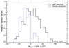 |
Fig. 5 Relative number of galaxies per bin for the Nançay and Arecibo samples as a function of the difference in W20 with fit to the W20−Lr relationship, i.e., W20−2.355 ·Lr0.207 with a bin size of 10. |
To see if this difference in Hi line profile width corresponds to any differences in over-all stellar distribution, we examine the distributions of r-band half-light radius. Here we define the half-light radius as the R50 radius encompassing 50% of the Petrosian flux, scaled for the Hubble-flow distance to the galaxy. This radius gives a general sense of the stellar mass concentration within a galaxy under the assumption that the mass-to-light ratios of galaxies of the same luminosity are fairly consistent. To test this assumption, we examined the distribution of g-r colors between the low luminosity (log(Lr) ≤ 8.5) Arecibo and NRT samples and found no significant difference (a Kolmogorov-Smirnov (K-S) test returns a 49.4% probability that these distributions are not drawn from the same parent sample). The similarities in color distribution between the two samples indicates that they do not have vastly differing stellar populations. Therefore, differences in half-light radius should indicate differences in compactness.
We plot the half-light radius distribution of the two samples in Fig. 6, which shows that the Arecibo data are systematically offset to lower radii than the Nançay data. The mean and standard deviations are 0.68 ± 0.32 kpc for Nançay and 0.47 ± 0.22 kpc for Arecibo. A K-S test returns a 94% probability that the Nançay and Arecibo samples are not drawn from the same parent distribution.
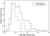 |
Fig. 6 Relative number of galaxies per bin of the Nançay and Arecibo samples as a function of half-light radius, in kpc. Bin size is 100 pc. |
The smaller half-light radii of the Arecibo sample, combined with the fact that these galaxies have narrower Hi line widths, on average, may indicate that these galaxies are indeed more compact. Since dwarf galaxies tend to have rotation curves that increase with radius, the narrow Hi line widths of these galaxies may be an indicator that the Hi is being confined to the central regions of the galaxy. If this is the case, it may imply that these galaxies are in a different phase of evolution than their Nançay detected counterparts. However, further investigation is necessary.
Basic optical and Hi data – Arecibo detected galaxies not included in the final Nançay sample.
In Fig. 7 we show the integrated Hi line flux as a function of the W50 line width for both our Arecibo and Nançay non-confused and non-resolved detections and marginals, together with the ALFALFA detections and marginals from Haynes et al. (2011) for comparison. We also indicate the line flux for a flat-topped 3σ detection with the mean Arecibo rms noise level of 0.57 mJy, to show where weak detections are expected to lie.
The ALFALFA data show an increasingly marked absence of weak sources with decreasing line width, beginning at about W50~ 100 km s-1. This is to due to both the detection threshold of ALFALFA (see Giovanelli et al. 2005) and the fact that blind surveys have no a priori knowledge of source redshifts. In the NIBLES observations, prior knowledge of the source redshift enables us to identify signals to a lower SNR.
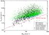 |
Fig. 7 Integrated Hi line flux FHI (in Jy km s-1) as a function of W50 line width (in km s-1). Shown are the NIBLES non-confused and non-resolved detections and marginals from both our Arecibo and Nançay observations, together with the ALFALFA data from the α.40 catalog (Haynes et al. 2011), where green dots represent detections (their Category 1) and light blue dots represent marginals (Category 2). The red line indicates the integrated line flux from a 3σ flat-topped profile with a 0.57 mJy rms noise level. |
Figure 8 shows Hi masses as a function of radial velocity for the same sources shown in Fig. 7. Additionally, we recalculated the Hi masses of the ALFALFA galaxies using pure Hubble-flow distances in order to maintain consistency with the NIBLES calculations. The green vertical arrow represents the 0.16 dex average offset in Hi mass due to difference in flux scale between the α.40 catalog and our NRT data discussed in Paper I.
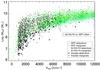 |
Fig. 8 Total Hi mass, MHI (in M⊙), as a function of Hi radial velocity (in km s-1). Shown are the NIBLES detections and marginals from both our Arecibo and Nançay observations (black stars and dots respectively), together with data based on the ALFALFA α.40 catalog (Haynes et al. 2011), where green dots represent detections (their Category 1) and light blue dots represent marginals (Category 2). Excluded were all NIBLES detections which are definitely or probably confused by another galaxy within the telescope beam, as well as detections that are likely resolved (see Paper I). The Hi masses of the ALFALFA detections were calculated in the same way as for the NIBLES sources, using simply a distance of D = V/H0, where the adopted Hubble constant is H0 = 70 km s-1 Mpc-1. The green vertical arrow above the legend indicates the difference of 0.16 in log(MHI) corresponding to the mean Hi flux scale difference between the α.40 catalog and our NRT data. |
In Fig. 9 we compare the Hi mass fraction log(MHI/M⋆) as a function of stellar mass (log(M⋆)), showing our Nançay (NRT) detections and marginals, ALFALFA detections, and our Arecibo sample detections, marginals, and upper limits for the non-detections. Our Arecibo upper limits were calculated following the same method used in Paper I, i.e., using a line width estimate from the upper envelope of the W20−Lr relationship. For ALFALFA, we also took the stellar mass estimates from the DR9 added-value MPA-JHU catalogs for consistency with the NIBLES sample (see Paper I).
The distribution of log(MHI/M⋆) vs. log(M⋆) data shows the same general trend as presented in Paper I and Papastergis et al. (2012), with the Hi-selected galaxy samples lying at systematically higher Hi mass fractions for a given stellar mass than the optically selected NIBLES galaxies. We note that Papastergis et al. (2012) used their own method for estimating the stellar masses of their sample (see Huang et al. 2012, for details). As mentioned in Paper I, the ALFALFA fluxes are systematically higher than ours by a factor of 1.45 due to flux scale differences (see the 0.16 dex vertical green arrow in Fig. 9). However, even taking this offset into account, the Hi-selected sample is has systematically higher MHI/M⋆ratios for a given M⋆than NIBLES.
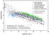 |
Fig. 9 Hi mass fraction (MHI/M⋆) as a function of total stellar mass, M⋆(in M⊙). NIBLES Nançay detections and marginals are represented by gray dots and open circles respectively while ALFALFA detections are represented by green dots. Our follow-up Arecibo detections and marginals are represented by solid and open light blue stars respectively while upper limits for non-detections are shown as downward arrows. Stellar masses used were taken from the SDSS added-value MPA-JHU catalogs (see Sect. 4). The green arrow below the legend represents the 0.16 dex average offset between the ALFALFA and NIBLES Hi masses due to flux scale differences and the black cross indicates the average uncertainty in the stellar masses and mass fractions (about 20% in both cases). The magenta line represents the fit to literature reference samples of Hi-detected galaxies from Papastergis et al. (2012), the blue and red lines represent the regression fits to the Nançay and Arecibo sources, respectively, which include estimated upper limits to Hi masses of undetected galaxies (see Paper I for further details). |
To assess the parameter space probed by our Arecibo sample, we also compare the literature fit made in Papastergis et al. (2012) of the four reference samples with Hi detections they used to evaluate the gas-to-stellar mass ratios of local galaxies (magenta), with fits to our data. We used the Buckley-James method of linear regression, taking into account the Hi non-detections, from the STSDAS statistics package1 to fit the Nançay (blue line) and Arecibo (red line) samples (see also Paper I). Since the log(MHI/M⋆) vs. log(M⋆) relationship becomes non-linear below log(M⋆) ~ 107.5, we only include masses above this cut-off in our fits. Average uncertainties for each Arecibo source are represented by the cross below the legend. We estimate a mean 1σ stellar mass uncertainty of about 20%, based on Kauffmann et al. (2003), and a typical uncertainty of about 20% for the NIBLES Arecibo gas mass fractions. Our typical gas mass fraction uncertainty for the entire NIBLES sample is about 27% (see Paper I for details).
As mentioned in Paper I, there is an increasing discrepancy between the Papastergis et al. (2012) reference sample Hi mass fraction (magenta) and the Nançay mass fraction (blue) as a function of increasing stellar mass. When comparing our Arecibo sample to the Nançay and Papastergis et al. (2012) samples, we see the Arecibo sample follows roughly the same trend as the Nançay data but with an approximately 0.5 dex offset toward lower Hi mass fractions. From Paper I, the Nançay regression fit is log(MHI/M⋆) = −0.59 log(M⋆) + 5.05 and the Arecibo fit is log(MHI/M⋆) = −0.65 log(M⋆) + 5.06. Since the Arecibo sample is a small fraction of the total NIBLES sample, we only show this fit here to illustrate the differences in Hi mass fractions of the Nançay undetected sample. If this trend is representative of the rest of the NIBLES Nançay undetected galaxies, we would expect the NRT regression fit to be offset toward lower mass fractions by about 0.17 dex. Taking the entire stellar mass range into account and comparing mean Hi mass fraction values in 0.2 mag wide bins in log(M⋆), we find that on average the Arecibo sample probes mass fractions that are 0.5 and 1 dex lower in log(MHI) than the Nançay and ALFALFA detections, respectively.
6. Conclusions
We obtained about four times more sensitive follow-up Hi observations at Arecibo of 90 NIBLES galaxies that were either not detected or marginally detected at Nançay. We detected 80% of these sources, which has enabled us to probe their underlying Hi distribution. The Arecibo detections have on average five times lower Hi masses than the Nançay upper limits estimated in Paper I. Contributing to this factor of five lower mass is not only the lower peak flux densities we are able to detect with Arecibo, but also the ~37% narrower line widths in our follow-up sample compared to the Nançay detections of sources with the same optical luminosity. This average difference in line width is primarily driven by the low luminosity (Lr< 108.5L⊙) sources which correspondingly show a higher central concentration of light. This may be an indication that these relatively gas-poor galaxies have, on average, a more centrally confined Hi mass distribution compared to the Nançay detected sample in the same luminosity range.
If we assume the g−i color and Lr distribution of Arecibo detection fractions are representative of the entire Nançay undetected and marginally detected samples, we estimate ~60% (520) could be detected with the four times better sensitivity of our Arecibo observations. This would put the over-all NIBLES detection rate at about 86%.
Lastly, our Arecibo follow-up observations enabled us to sample our Nançay undetected sample to Hi mass fractions 0.5 dex lower, on average, than our Nançay detections. Some of these galaxies with low MHI/M⋆ fractions lie in virtually unexplored parameter space (e.g., around log(Lr) = 11.5) and could potentially be used to shed further light on galaxy evolution processes studied by modelers, e.g., Kannappan et al. (2013).
Acknowledgments
The Arecibo Observatory is operated by SRI International under a cooperative agreement with the National Science Foundation (AST-1100968), and in alliance with Ana G. Méndez-Universidad Metropolitana, and the Universities Space Research Association. The Nançay Radio Telescope is operated as part of the Paris Observatory, in association with the Centre National de la Recherche Scientifique (CNRS) and partially supported by the Région Centre in France. This research has made use of the HyperLeda database (http://leda.univ-lyon1.fr), the NASA/IPAC Extragalactic Database (NED) which is operated by the Jet Propulsion Laboratory, California Institute of Technology, under contract with the National Aeronautics and Space Administration, and the Sloan Digital Sky Survey which is managed by the Astrophysical Research Consortium for the Participating Institutions.
References
- Benson, A. J., Bower, R. G., Frenk, C. S., et al. 2003, ApJ, 599, 38 [NASA ADS] [CrossRef] [Google Scholar]
- Blanton, M. R., & Collaboration, S. 2001, AJ, 121, 2358 [NASA ADS] [CrossRef] [Google Scholar]
- Blanton, M. R., Hogg, D. W., Brinkmann, J., et al. 2003, ApJ, 592, 819 [NASA ADS] [CrossRef] [Google Scholar]
- Briggs, F., Sorar, E., Kraan-Korteweg, R., & Van Driel, W. 1997, PASA, 14, 37 [Google Scholar]
- Brinchmann, J., Charlot, S., White, S. D. M., et al. 2004, MNRAS, 351, 1151 [NASA ADS] [CrossRef] [Google Scholar]
- de Vaucouleurs, G., de Vaucouleurs, A., Corwin, Jr., H. G., et al. 1991, Third Reference Catalogue of Bright Galaxies, Vol. I: Explanations and references, Vol. II: Data for galaxies between 0h and 12h, Vol. III: Data for galaxies between 12h and 24h (Springer-Verlag) [Google Scholar]
- Efstathiou, G., Ellis, R. S., & Peterson, B. A. 1988, MNRAS, 232, 431 [NASA ADS] [CrossRef] [Google Scholar]
- Felten, J. E. 1985, Comments on Astrophysics, 11, 53 [Google Scholar]
- Gavazzi, G., Fumagalli, M., Cucciati, O., & Boselli, A. 2010, A&A, 517, A73 [NASA ADS] [CrossRef] [EDP Sciences] [Google Scholar]
- Gehrels, N. 1986, ApJ, 303, 336 [NASA ADS] [CrossRef] [Google Scholar]
- Giovanelli, R., Haynes, M. P., Kent, B. R., et al. 2005, AJ, 130, 2613 [NASA ADS] [CrossRef] [Google Scholar]
- Haynes, M. P., Giovanelli, R., Martin, A. M., et al. 2011, AJ, 142, 170 [NASA ADS] [CrossRef] [Google Scholar]
- Hoppmann, L., Staveley-Smith, L., Freudling, W., et al. 2015, MNRAS, 452, 3726 [NASA ADS] [CrossRef] [Google Scholar]
- Huang, S., Haynes, M. P., Giovanelli, R., & Brinchmann, J. 2012, ApJ, 756, 113 [NASA ADS] [CrossRef] [Google Scholar]
- Kannappan, S. J., Stark, D. V., Eckert, K. D., et al. 2013, ApJ, 777, 42 [NASA ADS] [CrossRef] [Google Scholar]
- Kauffmann, G., Heckman, T. M., White, S. D. M., et al. 2003, MNRAS, 341, 33 [NASA ADS] [CrossRef] [Google Scholar]
- Kilborn, V., Webster, R. L., & Staveley-Smith, L. 1999, PASA, 16, 8 [NASA ADS] [CrossRef] [Google Scholar]
- Kovac, K., Oosterloo, T. A., & van der Hulst, J. M. 2005, Near-fields cosmology with dwarf elliptical galaxies, eds. H. Jerjen, & B. Binggeli, in IAU Colloq., 198, 351 [Google Scholar]
- Loveday, J., Peterson, B. A., Efstathiou, G., & Maddox, S. J. 1992, ApJ, 390, 338 [NASA ADS] [CrossRef] [Google Scholar]
- Loveday, J., Norberg, P., Baldry, I. K., et al. 2015, MNRAS, 451, 1540 [NASA ADS] [CrossRef] [Google Scholar]
- Lu, Y., Mo, H. J., Lu, Z., Katz, N., & Weinberg, M. D. 2014, MNRAS, 443, 1252 [NASA ADS] [CrossRef] [Google Scholar]
- Martin, A. M., Papastergis, E., Giovanelli, R., et al. 2010, ApJ, 723, 1359 [NASA ADS] [CrossRef] [Google Scholar]
- McNaught-Roberts, T., Norberg, P., Baugh, C., et al. 2014, MNRAS, 445, 2125 [NASA ADS] [CrossRef] [Google Scholar]
- Montero-Dorta, A. D., & Prada, F. 2009, MNRAS, 399, 1106 [NASA ADS] [CrossRef] [Google Scholar]
- Papastergis, E., Cattaneo, A., Huang, S., Giovanelli, R., & Haynes, M. P. 2012, ApJ, 759, 138 [NASA ADS] [CrossRef] [Google Scholar]
- Saintonge, A. 2007, AJ, 133, 2087 [NASA ADS] [CrossRef] [Google Scholar]
- Salim, S., Rich, R. M., Charlot, S., et al. 2007, ApJS, 173, 267 [NASA ADS] [CrossRef] [Google Scholar]
- Schechter, P. 1976, ApJ, 203, 297 [Google Scholar]
- Schlegel, D. J., Finkbeiner, D. P., & Davis, M. 1998, ApJ, 500, 525 [NASA ADS] [CrossRef] [Google Scholar]
- Schneider, S. E., Helou, G., Salpeter, E. E., & Terzian, Y. 1986, AJ, 92, 742 [NASA ADS] [CrossRef] [Google Scholar]
- Schneider, S. E., Thuan, T. X., Magri, C., & Wadiak, J. E. 1990, ApJS, 72, 245 [NASA ADS] [CrossRef] [Google Scholar]
- Springob, C. M., Haynes, M. P., & Giovanelli, R. 2005, ApJ, 621, 215 [NASA ADS] [CrossRef] [Google Scholar]
- Tremonti, C. A., Heckman, T. M., Kauffmann, G., et al. 2004, ApJ, 613, 898 [NASA ADS] [CrossRef] [Google Scholar]
- van Driel, W., Butcher, Z., Schneider, S., et al. 2016, A&A, 595, A118 (Paper I) [Google Scholar]
- Wilson, T. L., Rohlfs, K., & Huttemeister, S. 2009, Tools of Radio Astronomy (Springer-Verlag) [Google Scholar]
- York, D. G., Adelman, J., Anderson, Jr., J. E., et al. 2000, AJ, 120, 1579 [Google Scholar]
- Zwaan, M. A., Briggs, F. H., Sprayberry, D., & Sorar, E. 1997, ApJ, 490, 173 [NASA ADS] [CrossRef] [Google Scholar]
- Zwaan, M. A., Staveley-Smith, L., Koribalski, B. S., et al. 2003, AJ, 125, 2842 [NASA ADS] [CrossRef] [Google Scholar]
Appendix A: Baseline derippling
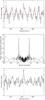 |
Fig. A.1 Illustration of the removal of a baseline ripple, in source 1260. a) Original observed Hi line spectrum, flux density (mJy) as a function of heliocentric velocity with the standing wave over-layed in red. b) Spectral power density (mJy/period) vs. period for the Fourier transform where the spikes in power density corresponding to 78 channels due to the baseline ripple are clearly much higher than the rest of the spectrum. c) The reverse Fourier transform of b) with the 78 channel period peaks removed. The standing wave has clearly been eliminated from the spectrum and the source signal is now easily identified. The vertical magenta dashed line indicates the SDSS optical velocity. This illustration represents one of two cases in our sample where this procedure was used. Source 1260 contained the stronger of the two standing waves. |
Two of our sources, 1260 and 2434 (i.e., PGC 4546173 and CGCG 427-032), suffered from a baseline ripple with a wavelength of approximately 210 km s-1 due to reflected radiation in the telescope structure (see Briggs et al. 1997; Wilson et al. 2009). At Arecibo, this effect is caused by the formation of a standing wave between the primary mirror and receiver cabin. It can be caused by a number of phenomena but is typically the result of a strong continuum source or broadband terrestrial RFI. The ripple shows up in the spectrum as a result of a slight phase variation between the ON and OFF scans. In Fourier space, this manifests itself as a narrow spike corresponding to a period across 78 correlator channels or a wavelength of ~300 m (frequency of ~1 MHz). This is wavelength is exactly what one would expect to see in a standing wave since they form in multiples of half-wavelength distances between two reflecting surfaces. The distance between the primary mirror and the receiver cabin is 150 m.
To illustrate this phenomenon, in Fig. A.1a we show the spectrum of source 1260 as it originally appeared with the standing wave easily apparent, which we have over-layed in red for reference. The Fourier transform (Fig. A.1b) shows the effect of the ripple as two clearly identifiable spikes. After removing the offending period and doing an inverse Fourier transform (Fig. A.1c), the source signal is much more easily identified, resulting in a detection.
Appendix B: Arecibo spectra
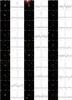 |
Fig. B.1 Color (g,r and i band composite) images from the SDSS alongside 21-cm Hi line spectra of galaxies clearly detected at Arecibo. The size of each image is 2′× 2′ with the NIBLES source number indicated in the upper left corner, absolute z-band magnitude, Mz, in the top center and log(MHI) in M⊙ in the top right corner of each image. The vertical axis in the spectra is flux density in mJy, the horizontal axis is heliocentric radial velocity (cz) in km s-1. The SDSS recession velocity is denoted by a vertical dashed magenta line, the mean Hi velocity by the blue triangle, and the W50 line width by the horizontal blue arrow bar. Confused galaxies are denoted by their confusion code from Sect. 4 in the upper right portion of the spectrum. Velocity resolution is 18.7 km s-1. |
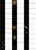 |
Fig. B.1 continued. |
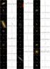 |
Fig. B.1 continued. |
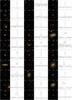 |
Fig. B.1 continued. |
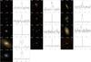 |
Fig. B.1 continued. |
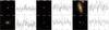 |
Fig. B.2 Color images from the SDSS alongside the 21-cm Hi line spectra of galaxies marginally detected at Arecibo. See Fig. B.1 for further details. |
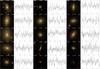 |
Fig. B.3 Color images from the SDSS alongside the 21-cm Hi line spectra of galaxies undetected at Arecibo. See Fig. B.1 for further details. |
All Tables
Basic optical and Hi data – Arecibo detections of Nançay non-detections and marginals.
Basic optical and Hi data – Arecibo marginal detections of Nançay non-detections.
Basic optical and Hi data – Arecibo detected galaxies not included in the final Nançay sample.
All Figures
|
Fig. 1 Number of galaxies as a function of g−i color, corrected for Galactic extinction following Schlegel et al. (1998). The black line is the total number of observed galaxies in each 0.25 mag wide bin and the blue line the total number of detected galaxies. The peak around 0.5 mag is due to our specific selection of blue objects (see Sect. 2). |
| In the text | |
|
Fig. 2 Integrated g−i color, in mag, as function of absolute r-band luminosity, log(Lr) in L⊙, both corrected for Galactic extinction following Schlegel et al. (1998). Nançay detections, marginals, and non-detections are represented by gray dots, open gray circles, and open red circles respectively. Arecibo detections, marginals, and non-detections are respectively represented by black solid stars, open stars, and blue downward triangles. The low luminosity end (log(Lr) <9) shows a color dichotomy with Hi detections and non-detections clustering around g−i ~ 0.4 and g−i ~ 0.8 respectively, showing a clear distinction between the blue cloud and red sequence galaxies. Above luminosities of log(Lr) ~ 9.5, the blue cloud disappears while the red sequence galaxies shift to redder colors, g−i ~ 1.2. |
| In the text | |
|
Fig. 3 a) Detection fraction for the NIBLES Nançay sample (gray) and the Arecibo follow-up sample (black) as a function of g−i color. b) Detection fractions as a function of r-band luminosity. Error bars for the Nançay data are the standard deviation of the binomial distribution and the error bars for the Arecibo data were calculated following Gehrels (1986) using the 90% confidence intervals. Bin sizes are 0.3 for a) and 1 for b). |
| In the text | |
|
Fig. 4 Total number of galaxies either undetected or marginally detected at Nançay that would be detectable with the same sensitivity as our Arecibo observations, as a function of g−i color. Black indicates Nançay non-detections and marginals, whereas the solid blue line is the estimated number of galaxies that would be detectable based on our Arecibo sample detection rate. The blue dashed and dash-dotted lines are based on, respectively, the upper and lower envelopes of the uncertainties in the detection rate, see Fig. 3. |
| In the text | |
|
Fig. 5 Relative number of galaxies per bin for the Nançay and Arecibo samples as a function of the difference in W20 with fit to the W20−Lr relationship, i.e., W20−2.355 ·Lr0.207 with a bin size of 10. |
| In the text | |
|
Fig. 6 Relative number of galaxies per bin of the Nançay and Arecibo samples as a function of half-light radius, in kpc. Bin size is 100 pc. |
| In the text | |
|
Fig. 7 Integrated Hi line flux FHI (in Jy km s-1) as a function of W50 line width (in km s-1). Shown are the NIBLES non-confused and non-resolved detections and marginals from both our Arecibo and Nançay observations, together with the ALFALFA data from the α.40 catalog (Haynes et al. 2011), where green dots represent detections (their Category 1) and light blue dots represent marginals (Category 2). The red line indicates the integrated line flux from a 3σ flat-topped profile with a 0.57 mJy rms noise level. |
| In the text | |
|
Fig. 8 Total Hi mass, MHI (in M⊙), as a function of Hi radial velocity (in km s-1). Shown are the NIBLES detections and marginals from both our Arecibo and Nançay observations (black stars and dots respectively), together with data based on the ALFALFA α.40 catalog (Haynes et al. 2011), where green dots represent detections (their Category 1) and light blue dots represent marginals (Category 2). Excluded were all NIBLES detections which are definitely or probably confused by another galaxy within the telescope beam, as well as detections that are likely resolved (see Paper I). The Hi masses of the ALFALFA detections were calculated in the same way as for the NIBLES sources, using simply a distance of D = V/H0, where the adopted Hubble constant is H0 = 70 km s-1 Mpc-1. The green vertical arrow above the legend indicates the difference of 0.16 in log(MHI) corresponding to the mean Hi flux scale difference between the α.40 catalog and our NRT data. |
| In the text | |
|
Fig. 9 Hi mass fraction (MHI/M⋆) as a function of total stellar mass, M⋆(in M⊙). NIBLES Nançay detections and marginals are represented by gray dots and open circles respectively while ALFALFA detections are represented by green dots. Our follow-up Arecibo detections and marginals are represented by solid and open light blue stars respectively while upper limits for non-detections are shown as downward arrows. Stellar masses used were taken from the SDSS added-value MPA-JHU catalogs (see Sect. 4). The green arrow below the legend represents the 0.16 dex average offset between the ALFALFA and NIBLES Hi masses due to flux scale differences and the black cross indicates the average uncertainty in the stellar masses and mass fractions (about 20% in both cases). The magenta line represents the fit to literature reference samples of Hi-detected galaxies from Papastergis et al. (2012), the blue and red lines represent the regression fits to the Nançay and Arecibo sources, respectively, which include estimated upper limits to Hi masses of undetected galaxies (see Paper I for further details). |
| In the text | |
|
Fig. A.1 Illustration of the removal of a baseline ripple, in source 1260. a) Original observed Hi line spectrum, flux density (mJy) as a function of heliocentric velocity with the standing wave over-layed in red. b) Spectral power density (mJy/period) vs. period for the Fourier transform where the spikes in power density corresponding to 78 channels due to the baseline ripple are clearly much higher than the rest of the spectrum. c) The reverse Fourier transform of b) with the 78 channel period peaks removed. The standing wave has clearly been eliminated from the spectrum and the source signal is now easily identified. The vertical magenta dashed line indicates the SDSS optical velocity. This illustration represents one of two cases in our sample where this procedure was used. Source 1260 contained the stronger of the two standing waves. |
| In the text | |
|
Fig. B.1 Color (g,r and i band composite) images from the SDSS alongside 21-cm Hi line spectra of galaxies clearly detected at Arecibo. The size of each image is 2′× 2′ with the NIBLES source number indicated in the upper left corner, absolute z-band magnitude, Mz, in the top center and log(MHI) in M⊙ in the top right corner of each image. The vertical axis in the spectra is flux density in mJy, the horizontal axis is heliocentric radial velocity (cz) in km s-1. The SDSS recession velocity is denoted by a vertical dashed magenta line, the mean Hi velocity by the blue triangle, and the W50 line width by the horizontal blue arrow bar. Confused galaxies are denoted by their confusion code from Sect. 4 in the upper right portion of the spectrum. Velocity resolution is 18.7 km s-1. |
| In the text | |
|
Fig. B.1 continued. |
| In the text | |
|
Fig. B.1 continued. |
| In the text | |
|
Fig. B.1 continued. |
| In the text | |
|
Fig. B.1 continued. |
| In the text | |
|
Fig. B.2 Color images from the SDSS alongside the 21-cm Hi line spectra of galaxies marginally detected at Arecibo. See Fig. B.1 for further details. |
| In the text | |
|
Fig. B.3 Color images from the SDSS alongside the 21-cm Hi line spectra of galaxies undetected at Arecibo. See Fig. B.1 for further details. |
| In the text | |
Current usage metrics show cumulative count of Article Views (full-text article views including HTML views, PDF and ePub downloads, according to the available data) and Abstracts Views on Vision4Press platform.
Data correspond to usage on the plateform after 2015. The current usage metrics is available 48-96 hours after online publication and is updated daily on week days.
Initial download of the metrics may take a while.