| Issue |
A&A
Volume 596, December 2016
|
|
|---|---|---|
| Article Number | A67 | |
| Number of page(s) | 21 | |
| Section | Extragalactic astronomy | |
| DOI | https://doi.org/10.1051/0004-6361/201527947 | |
| Published online | 01 December 2016 | |
SN 2012aa: A transient between Type Ibc core-collapse and superluminous supernovae
1 The Oskar Klein Centre, Department of Astronomy, Stockholm University, AlbaNova, 10691 Stockholm, Sweden
e-mail: rupak.roy@astro.su.se; rupakroy1980@gmail.com
2 Department of Astronomy, University of Texas, Austin, TX 78712-0259, USA
3 INAF−Osservatorio Astronomico di Padova, Vicolo dell’Osservatorio 5, 35122 Padova, Italy
4 California Institute of Technology, 1200 E. California Blvd., CA 91225, USA
5 Astrophysics Research Centre, School of Mathematics and Physics, Queen’s University Belfast, BT7 1NN, UK
6 Indian Institute of Astrophysics, Koramangala, 560 034 Bangalore, India
7 Aryabhatta Research Institute of Observational Sciences (ARIES), Manora Peak, 263 129 Nainital, India
8 Department of Astronomy, University of California, Berkeley, CA 94720-3411, USA
9 Department of Physics, University of California, Davis, CA 95616-8677, USA
10 Harvard-Smithsonian Center for Astrophysics, 60 Garden Street, Cambridge, MA 02138, USA
11 Instituto de Astrofísica de Canarias, 38205 La Laguna, Tenerife, Spain
12 Dpto. de Astrofísica, Universidad de La Laguna, 38206 La Laguna, Tenerife, Spain
13 Grantecan CALP, 38712, Bren̅a Baja, La Palma, Spain
Received: 11 December 2015
Accepted: 1 July 2016
Context. Research on supernovae (SNe) over the past decade has confirmed that there is a distinct class of events which are much more luminous (by ~2 mag) than canonical core-collapse SNe (CCSNe). These events with visual peak magnitudes ≲–21 are called superluminous SNe (SLSNe). The mechanism that powers the light curves of SLSNe is still not well understood. The proposed scenarios are circumstellar interaction, the emergence of a magnetar after core collapse, or disruption of a massive star through pair production.
Aims. There are a few intermediate events which have luminosities between these two classes. They are important for constraining the nature of the progenitors of these two different populations and their environments and powering mechanisms. Here we study one such object, SN 2012aa.
Methods. We observed and analysed the evolution of the luminous Type Ic SN 2012aa. The event was discovered by the Lick Observatory Supernova Search in an anonymous galaxy (z ≈ 0.08). The optical photometric and spectroscopic follow-up observations were conducted over a time span of about 120 days.
Results. With an absolute V-band peak of ~− 20 mag, the SN is an intermediate-luminosity transient between regular SNe Ibc and SLSNe. SN 2012aa also exhibits an unusual secondary bump after the maximum in its light curve. For SN 2012aa, we interpret this as a manifestation of SN-shock interaction with the circumstellar medium (CSM). If we assume a 56Ni-powered ejecta, the quasi-bolometric light curve requires roughly 1.3 M⊙ of 56Ni and an ejected mass of ~14M⊙. This also implies a high kinetic energy of the explosion, ~5.4 × 1051 erg. On the other hand, the unusually broad light curve along with the secondary peak indicate the possibility of interaction with CSM. The third alternative is the presence of a central engine releasing spin energy that eventually powers the light curve over a long time. The host of SN 2012aa is a star-forming Sa/Sb/Sbc galaxy.
Conclusions. Although the spectral properties of SN 2012aa and its velocity evolution are comparable to those of normal SNe Ibc, its broad light curve along with a large peak luminosity distinguish it from canonical CCSNe, suggesting that the event is an intermediate-luminosity transient between CCSNe and SLSNe at least in terms of peak luminosity. In comparison to other SNe, we argue that SN 2012aa belongs to a subclass where CSM interaction plays a significant role in powering the SN, at least during the initial stages of evolution.
Key words: supernovae: general / supernovae: individual: SN 2012aa
© ESO, 2016
1. Introduction
The study of superluminous supernovae (SLSNe; Gal-Yam 2012) has emerged from the development of untargeted transient surveys such as the Texas Supernova Search (Quimby 2006), the Palomar Transient Factory (PTF; Rau et al. 2009), the Catalina Real-time Transient Survey (CRTS; Drake et al. 2009), and the Panoramic Survey Telescope & Rapid Response System (Pan-STARRS; Hodapp et al. 2004). SLSNe are much more luminous than normal core-collapse SNe (CCSNe; Filippenko 1997). It was with the discovery of objects such as SNe 2005ap and SCP-06F6 (Quimby et al. 2007, 2011) as well as SN 2007bi (Gal-Yam et al. 2009) that events with peak luminosities ≳7 × 1043 erg s-1 (≲− 21 absolute mag, over 2 mag brighter than the bulk CCSN population) became known.
SLSNe have been classified into three groups: SLSN-I, SLSN-II, and SLSN-R (Gal-Yam 2012). The SLSN-II are hydrogen (H)-rich (e.g., SN 2006gy, Smith et al. 2007; CSS100217, Drake et al. 2011; CSS121015, Benetti et al. 2014), while the others are H-poor. The SLSN-R (e.g., SN 2007bi, Gal-Yam et al. 2009) have post-maximum decline rates consistent with the 56Co →56Fe radioactive decay, whereas SLSNe-I (e.g., SNe 2010gx, Pastorello et al. 2010b; SCP-06F6) have steeper declines. Hydrogen-poor events mostly exhibit SN Ic-like spectral evolution (Pastorello et al. 2010b; Quimby et al. 2011; Inserra et al. 2013). However, the explosion and emission-powering mechanisms of these transients are still disputed. It is also not clear whether CCSNe and SLSNe originated from similar or completely different progenitor channels, or if there is a link between these kinds of explosions. In particular, the SLSNe-R were initially thought to be powered by radioactive decay, but later the energy release of a spin-down magnetar was proposed (Inserra et al. 2013), as was the CSM-interaction scenario (Yan et al. 2015; Sorokina et al. 2016). In this work, although we use the notation of the initial classification scheme, by SLSNe-R we simply mean those Type Ic SLSNe which show shallow (or comparable to 56Co decay) decline after maximum brightness, while the events which decline faster than 56Co decay are designated SLSNe-I.
The basic mechanisms governing the emission of stripped-envelope CCSNe are relatively well known. At early times (≲5 d after explosion), SNe Ibc are powered by a cooling shock Piro & Nakar (2013), Taddia et al. (2015). Thereafter, radioactive heating (56Ni →56Co) powers the emission from the ejecta. Beyond the peak luminosity, the photosphere cools and eventually the ejecta become optically thin. By ~100 d post explosion the luminosity starts to decrease linearly (in mag) with time, and it is believed that 56Co is the main source powering the light curve during these epochs (Arnett 1982, and references therein).
Three different models have been suggested for the explosion mechanism of SLSNe. A pair-instability supernova (PISN) produces a large mass of radioactive 56Ni, a source of enormous optical luminosity (Barkat et al. 1967; Rakavy & Shaviv 1967). Alternatively, a similarly large luminosity can be produced by interaction between the SN ejecta and a dense circumstellar medium (CSM) surrounding the progenitor, and the radiation is released when the strong shocks convert the bulk kinetic energy of the SN ejecta to thermal energy (Smith & McCray 2007; Chevalier & Irwin 2011; Ginzburg & Balberg 2012). The third alternative is to invoke an engine-driven explosion: a proto-magnetar is a compact remnant that radiates enormous power during its spin-down process (Kasen & Bildsten 2010; Woosley 2010). Although both magnetar engines and CSM interaction can reproduce the range of luminosities and shapes of SLSN light curves, there are very few SNe that show a PISN-like 56Co →56Fe decay rate after maximum light. Only ~10% of SLSNe show a slowly fading tail (Nicholl et al. 2013; McCrum et al. 2015; Chen et al. 2015), but do not exactly follow the radioactive decay rate of cobalt. SLSNe 2006gy and 2007bi could be explained as PISN producing ~5−10 M⊙ of 56Ni (Nomoto et al. 2007; Gal-Yam et al. 2009), but there are also counter-arguments that the rise times of some similar events are shorter than the PISN model predictions (Kasen et al. 2011; Moriya et al. 2013; Nicholl et al. 2013, and references therein).
Beyond the general evolutionary picture of Type I SNe (hereafter we exclude SNe Ia), many events exhibit different kinds of peculiarities. One of these, observed in SN 2005bf, is the appearance of a short-lived bump before the principal light-curve peak (Anupama et al. 2005). Two hypotheses have been proposed to explain this early short-duration bump: either a burst of radiation from a blob containing radioactive 56Ni that was ejected asymmetrically (Maeda et al. 2007) or a polar explosion powered by a relativistic jet (Folatelli et al. 2006). Although a double-peaked light curve was only observed in a single SN Ic, there are at least a handful (~8) of Type I SLSNe that exhibit a short-duration bump before the principal broad peak (Nicholl & Smartt 2016). Most of them have been described using the magnetar model. For SN-LSQ14bdq it was proposed that the intense radiation in optical and ultraviolet wavelengths was due to the emergence of the shock driven by a high-pressure bubble produced by the central engine, a proto-magnetar (Kasen et al. 2016).
Since H-poor SLSNe and normal Type Ic events show similar spectral features beyond maximum light, it is worth exploring whether there is any link between them. The gap between SNe and SLSNe has not been well explored. The Type Ib SN 2012au shows spectral signatures which mark the transition between H-poor CCSNe and SLSNe, although its peak magnitude was comparable to those of H-poor (stripped envelope) CCSNe (Milisavljevic et al. 2013). The luminosity of broad line Type Ic SN 2011kl, associated with GRB 111209A also fall in between CCSNe and SLSNe (Greiner et al. 2015; Kann et al. 2016). Recently, a few transients such as PTF09ge, PTF09axc, PTF09djl, PTF10iam, PTF10nuj, and PTF11glr with peak absolute magnitudes between − 19 and − 21 have been discovered (Arcavi et al. 2014). Except PTF09ge, all had H-dominated spectra, and except PTF10iam they showed spectral behaviour like that of tidal disruption events (TDEs; Rees 1988). However, we note that TDEs may be even more luminous than SLSNe; for example, the ROTSE collaboration found an event (nicknamed Dougie) that had a peak magnitude of ~− 22.5 (Vinkó et al. 2015). Unlike CCSNe or SLSNe, TDEs are always found at the center of their host galaxies, and their spectral features are normally dominated by H/He emission lines, thus differing from Type Ic SNe. Arcavi et al. (2016) also found four SNe having rapid rise times (~10 d) and peak magnitudes of ~− 20 along with an Hα signature in their spectra (see Sect. 9.3).
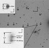 |
Fig. 1 Identification chart of SN 2012aa. The image is about 10′ on each side, taken in the Rc band with the 1.04 m Sampurnanand telescope at ARIES, Nainital. The local standard stars are numbered. North is up and east is to the left. The location of the target is marked “T”, as observed with the 8 m Gemini South telescope (bottom inset) on 2012 April 26, +88 d after discovery. The SN is resolved; its position and the host center are marked. The field was also observed with the 3 m TNG (top inset) on 2013 April 9, long after the SN had faded away. The SN location is not resolved in the TNG image. |
In this work, we discuss the evolution of a SN Ic that shows intermediate properties between those of SNe Ic and H-poor SLSNe. SN 2012aa (=PSN J14523348-0331540) was discovered on 2012 January 29.56 UT (JD 2 455 956.04) in a relatively distant anonymous galaxy (redshift z = 0.083; see Sect. 3) during the Lick Observatory Supernova Search (LOSS; Filippenko et al. 2001) with the Katzman Automatic Imaging Telescope (KAIT). An image of the field of SN 2012aa is shown in Fig. 1. Basic properties of the host galaxy are given in Table 1. The event was observed at ~17.7 mag (unfiltered) at discovery, and was further monitored in the subsequent nights and then spectroscopically classified as a SN Ic (Cenko et al. 2012) on February 2 (UT dates are used throughout this paper). It was not observed in the X-ray in radio domains. However, independent optical photometry along with spectroscopic follow-up observations were obtained using various telescopes around the globe. We find that the event was actually discovered near its peak (see Sect. 4), but it was caught in its rising phase by the CRTS survey (Drake et al. 2009). It shows some spectroscopic resemblance to H-poor SLSNe, although photometrically the peak is about 1 mag fainter than that of typical SLSNe. More remarkably, SN 2012aa shows an unusual secondary bump after a broad primary peak in its light curve (Sect. 4).
Properties of SN 2012aa and its host galaxy.
Here we present an optical photometric and low-resolution spectroscopic investigation of SN 2012aa. We also make comparisons among SN 2012aa, SLSNe, and CCSNe. The paper is organized as follows. Section 2 presents a brief description of the observations of SN 2012aa along with a description of the data reduction procedure. The distance and extinction are estimated in Sect. 3. In Sect. 4, we study the light-curve evolution, while the evolution of the colours and of the quasi-bolometric luminosity are discussed in Sect. 5. The spectroscopic evolution is presented in Sect. 6, and the properties of the host galaxy in Sect. 7. Section 8 explores different physical parameters of the explosion, and a comparative study of this event with SLSNe and CCSNe is given in Sect. 9. Finally, Sect. 10 summarizes our conclusions.
2. Observations and data reduction
2.1. Optical multiband photometry
The optical broadband Johnson BV and Cousins RcIc follow-up observations started on 2012 February 10, using the 1.04 m Sampurnanand Telescope (ST) plus imaging camera1 at Nainital, India, and were conducted at 17 different epochs between +12 d and +116 d after the discovery. The field was also observed in 3 epochs with the 1.82 m Copernico Telescope (CT) plus AFOSC at the Asiago Observatory and in 2 epochs with the 3.6 m New Technology Telescope (NTT) plus EFOSC2 at ESO, Chile, between +44 d and +93 d after discovery. The pre-processing was done using standard data reduction software IRAF2, and photometric measurements were performed on the coadded frames through point spread function (PSF) fitting and background-subtraction methods, using the stand-alone version of DAOPHOT3 (Stetson 1987). The field was calibrated in the BVRcIc bands using Landolt (1992) standard stars from the fields of SA107, PG1633+099, and PG1525+071 observed on 2014 April 27 under moderate seeing (full width at half maximum intensity (FWHM) ≈ 2′′ in the V band) and clear sky conditions4. Nine isolated non-variable stars (marked in Fig. 1) in the field of the transient were used as local standards to derive the zero point for the SN images at each epoch. The calibrated magnitudes of these nine secondary standards are given in Table 2.
Photometry of secondary standard stars in the field of SN 2012aa.
The SN was not resolved in the images taken with 1−3 m telescopes (see Fig. 1). The host along with the SN appeared as a point source (T) in all frames taken from ST and CT, while it slightly elongated in the NTT images. It was resolved only in the spectroscopic-acquisition image obtained with the Gemini-South telescope at +88 d after discovery under excellent seeing conditions ( ; see the bottom inset of Fig. 1). Performing astrometry on the image, we calculate the position of the host center as
  ,
,  , while that of the SN is
  ,
,  . The projected dimension (major axis) of the galaxy is ~
 , while the separation between the SN and the host center is ~
 in the plane of the sky. As most of the photometric observations have worse seeing than the separation between SN and host center, photometry of these images provides an estimate of the total flux of the entire system T (supernova plus host).
In order to calculate the magnitude of the transient, an estimate of the host magnitude is required. For this purpose, the field was again observed in the BVRcIc bands after the SN had faded, first on 2013 April 9 using the 3.5 m Telescopio Nazionale Galileo (TNG) plus the LRS camera, and then again on 2014 April 27, the night for the photometric calibration at ST. The Rc-band image taken with the TNG is shown in the top inset of Fig. 1. Aperture photometry (with an aperture diameter of ~) was performed to estimate the average magnitudes of the host: 20.17 ± 0.06, 19.29 ± 0.04, 18.67 ± 0.05, and 18.04 ± 0.04 mag in the B, V, Rc, and Ic bands, respectively. When determining the magnitude of the transient in every band, the flux of the host in the corresponding band was subtracted from the calibrated flux of T. The photometry of SN 2012aa is given in Table 3. Since the host is relatively distant, we calculated the K-correction term for every band at each epoch of observation using the existing spectra5 (Sect. 2.2). K-corrections for all photometric epochs are also given in Table 3.
BVRcIc photometry of SN 2012aa.
Journal of spectroscopic observations of SN 2012aa.
We have also used the unfiltered data taken from CRTS, which provide extensive coverage of the field. All the unfiltered CRTS magnitudes have been calibrated to the Johnson V band using the local sequences. The CRTS images have low spatial resolution (2.̋43 pixel-1). Photometry of all CRTS observations was performed in two different ways. Using flux subtraction, a calibrated template frame was produced after adding ten aligned CRTS images having moderate seeing (~2.̋5) and without the SN. Then the calibrated flux of the host from this “stacked template” was subtracted from all other CRTS measurements, in the same way as mentioned above for the photometry of other observations. With template subtraction, the “stacked template” is used as a reference image following standard procedures (e.g., Roy et al. 2011, and references therein). Comparison of the results of these two processes shows consistency (see Sect. 4). Photometry with flux subtraction is presented in Table A.1.
2.2. Low-resolution optical spectroscopy
Long-slit low-resolution spectra (~6−14 Å) in the optical range (0.35−0.95 μm) were collected at eight epochs between +4 d and +905 d after discovery. These include two epochs from the 3 m Shane reflector at Lick Observatory, two epochs from the 10 m Keck-I telescope, and one epoch each from the 2 m IUCAA Girawali Observatory (IGO, India), the 2.56 m Nordic Optical Telescope (NOT, La Palma), the 3.6 m NTT, and the 8 m Gemini-South telescope. All of the spectroscopic data were reduced under the IRAF environment6. All spectra of SN 2012aa were normalized with respect to the average continuum flux derived from the line-free region 6700−7000 Å. For the rest of the analysis we used the normalized spectra of the SN. The spectrum, obtained with NOT+ALFOSC on 2014 July 22 (+905d after discovery), contains mainly emission from the host. This flux-calibrated spectrum was utilized to quantify the host properties. The journal of spectroscopic observations is given in Table 4.
3. Distance and extinction toward SN 2012aa
The distance was calculated from the redshift of the host galaxy. The host spectrum (see Sect. 7, Fig. 12) contains strong emission lines of Hα, Hβ, [N ii ] λλ6548, 6583, [O ii ] λ3727, and [S ii ] λλ6717, 6731. Using these emission lines, the measured value of the redshift is 0.0830 ± 0.0005. This corresponds to a luminosity distance DL = 380 ± 2 Mpc using a standard cosmological model7, and hence the distance modulus (μ) is 37.9 ± 0.01 mag.
The extinction toward SN 2012aa is dominated by the Milky Way contribution. The Galactic reddening in the line of sight of SN 2012aa, as derived by Schlafly & Finkbeiner (2011), is E(B−V) = 0.088 ± 0.002 mag. The host contribution toward the SN can be estimated from theNa i D absorption line in spectra of the SN. We use the empirical relation between the equivalent width ofNa i D absorption and E(B−V) (Poznanski et al. 2012, and references therein).
In the SN spectra we did not detect any significantNa i D absorption at the rest wavelength of the host. The dip nearest to this wavelength has an equivalent width of 0.30 Å and is comparable to the noise level. This corresponds to E(B−V)≈ 0.032 mag and can be considered an upper limit for the contribution of the host to the reddening toward the SN.
Hence, an upper limit for the total reddening toward SN 2012aa is E(B−V)upper = 0.12 mag, while its lower limit is E(B−V)lower = 0.088 mag. We use E(B−V)upper as the total reddening toward the SN. This corresponds to a total visual extinction AV = 0.37 mag, adopting the ratio of total-to-selective extinction RV = 3.1.
4. Light-curve evolution of SN 2012aa
The optical photometric light curves are shown in Fig. 2 and the data are given in Table 3.
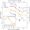 |
Fig. 2 Optical light curves of SN 2012aa. The BVRcIc photometric measurements from ST, CT, and NTT are shown respectively with filled circles, squares, and triangles, while the CRTS measurements are open circles. The epochs are given with respect to the date of discovery. All the unfiltered CRTS magnitudes have been calibrated to the Johnson V-filter system using the local sequences. The solid line represents a third-order polynomial fit around the first broad peak observed in V, while the dotted lines represent third-order polynomial fits around the secondary peak in BVRcIc. The inset represents a comparison between the measurements from CRTS observations by using template subtraction (open stars) and flux subtraction (open circles). The solid line around the peak is again a third-order polynomial fit around the first peak using the measurements obtained from template subtraction. It is worth noting that the absolute-magnitude scale is corrected only for distance modulus (μ) to show the approximate luminosity. When determining a more accurate luminosity, reddening and the K-correction were also considered. See text for details. |
The long-term photometry of the host recorded by CRTS is presented in Fig. 3. The photometric measurements of the CRTS images by the flux subtraction and template subtraction methods give consistent results (see the inset in Fig. 2). To maintain consistency in the reductions of all photometric observations, we adopt the results of the flux subtraction method in the rest of the work.
From the CRTS data it is clear that the explosion took place long before the discovery. SN 2012aa was actually discovered around its peak brightness. However, owing to the very sparse dataset before the peak, precise estimates of the epoch of maximum and the corresponding peak magnitude using polynomial fitting are difficult. A third-order polynomial fit to the V-band peak magnitudes (solid-line in Fig. 2) indicates that the epoch of V-band maximum was JD 2 455 9528, with MV ≈ −19.87 mag. The host V-band magnitude, measured from pre-SN CRTS data, is 19.11 mag (see Sect. 4.3). The polynomial fits to the combined V-band and CRTS data of SN 2012aa reach 19.11 mag roughly between 30−35 d prior to the discovery. Therefore, we assume that the event had a long rise time of ≳30 d.
4.1. Early evolution (<60 days after peak)
A slowly rising, broad light curve with a secondary peak makes this event special. The V-band light curve seems to rise to maximum on a similar timescale as it later declines after peak. Moreover, by fitting third-order polynomials to the BVRcIc light curves after +30 d, we find a rebrightening in all optical bands that produce a second peak (or bump) in the light curves appearing between ~+40 d and +60 d after the first V-band maximum. Beyond that, a nearly exponential decline of the optical light marks the onset of the light-curve tail. This kind of secondary bump in the light curve has been observed in a few other CCSNe, but is not common in SNe Ic. Different physical processes could explain these data, and a few scenarios are discussed below.
Objects that resemble SN 2012aa photometrically are the Type Ibn/IIn SNe 2005la (Pastorello et al. 2008) and 2011hw (Smith et al. 2012; Pastorello et al. 2015) and the SN Ibn iPTF13beo (Gorbikov et al. 2014), where double or multiple-peaked light curves were also reported. To some extent the light curves of the luminous Type IIn (or Type IIn-P) SNe 1994W (Sollerman et al. 1998) and 2009kn (Kankare et al. 2012) also exhibited similar features with relatively flat light curves during their early evolution. All of these were interpreted as being produced by SN shock interaction with the dense CSM. This proposition was supported by the appearance of strong, narrow H/He features in the SN spectra caused by electron scattering in the dense CSM during the interaction process (Chugai 2001; Smith et al. 2012; Fransson et al. 2014, and references therein). The pre-explosion outburst in the progenitor is the potential mechanism that can produce such dense CSM (Smith 2014). In fact, in a few luminous blue variables (LBVs) such pre-explosion outbursts have been recorded (e.g., Humphreys et al. 1999; Smith et al. 2010; Pastorello et al. 2013; Fraser et al. 2013; Ofek et al. 2014, and references therein). During its major event in 2012, the progenitor of SN 2009ip also exhibited a bump ~40 d after its first maximum, which was interpreted as an effect of shock interaction (Smith et al. 2014; Graham et al. 2014; see also Martin et al. 2015, and references therein). Similarly, SN 2010mb, which is spectroscopically very similar to SN 2012aa, is a rare example where interaction of a SN Ic with an H-free dense CSM was proposed (Ben-Ami et al. 2014).
However, the spectral sequence of SN 2012aa (see Sect. 6) shows that the effects of shock interaction are not prominent in its line evolution. The photometric behaviour of the SN must therefore be caused mainly by changes in the continuum flux.
Recently, Nicholl et al. (2015) made a comparative study between SLSNe I and SNe Ic with a sample of 21 objects. They computed the rise (τris) and decline (τdec) timescales, which were defined as the time elapsed before (or after) the epoch of maximum during which the SN luminosity rises to (or declines from) the peak luminosity from (or to) a value that is e-1 times its peak luminosity. This corresponds to a drop of 1.09 mag. Using these definitions and by fitting third-order polynomials around the first V maximum, we found τris ≈ 31 d and τdec ≈ 55 d for SN 2012aa. However, unlike the SLSNe discussed by Nicholl et al. (2015), SN 2012aa exhibits light curves with shallow decline after the peak followed by a secondary bump before entering the nebular phase. Therefore, we calculated the post-maximum decline rate (Rdec [mag d-1]) of this object in the rest frame to compare the nature of its light curves with those of other SNe. Here we simply assume that the secondary bump at ~+50 d is produced by another physical process.
For events (e.g., H-poor CCSNe) with Tneb ≳ τdec, we can consider  , where Tneb is the time (with respect to the time of maximum brightness) when the tail phase starts. The post-maximum decline rates (Rdec) of SN 2012aa in the BVRcIc bands (calculated between +15 d and +30 d) are ~0.03, 0.02, 0.01, and 0.02 mag d-1, respectively. These values are less than Rfall and are comparable to Rtail of broad-lined SNe Ic9. The post-maximum decline rates of SN 2012aa in the different bands are consistent with the values of τdec obtained by Nicholl et al. (2015) using the quasi-bolometric light curves of CCSNe, and are also similar to the SLSNe(-I) which decline quickly after maximum brightness (e.g., SNe 2010gx, 2011ke, 2011kf, PTF10hgi, PTF11rks), but are not comparable to SLSNe(-R) which have a slow decline after maximum (e.g., SNe 2007bi, 2011bm, PTF12dam, PS1-11ap). We discuss this further in Sect. 9.
4.1.1. Secondary bump in SN 2012aa
A second bump in the SN light curve beyond maximum brightness is not common among SNe Ibc. In SN 2012aa it was observed at ~50 d after the principal peak (i.e., ~80 d after the explosion, assuming a rise time of ≳30 d). In the simplest scenario, this secondary bump may be an effect of shock interaction with clumpy CSM having a jump in its density profile. Under the assumption that the typical SN shock velocity is ~104 km s-1, the region of the density jump should be located at a distance of ~1016 cm from the explosion site.
If the density jump is spherically symmetric around the SN location, it may be in the form of a dense shell, created from an eruption by the progenitor before the SN explosion. If we consider that the outward radial velocity of the erupted material is ~103 km s-1, we can estimate that in SN 2012aa, the putative pre-SN stellar eruption happened a few years prior to the final explosion. In the existing pre-SN data on SN 2012aa (Sect. 4.3) we could not find any significant rise in luminosity due to outburst as a precursor activity (see, e.g., Smith et al. 2010). This is, however, not surprising given that our observations are insensitive to the expected small variations and the stellar eruptions are of short duration, are quite unpredictable, and may happen at any time.
A secondary bump is also observed in the near-infrared light curves of Type Ia SNe, to some extent similar to the secondary bump in SN 2012aa. In SNe Ia this is caused by the transition ofFe iii ions toFe ii ions and is observable mainly at longer wavelengths (Kasen 2006). Unlike SNe Ia, SN 2012aa also exhibits a secondary bump in the B and V bands. This indicates that the generation mechanism for the secondary bumps in SN 2012aa is different from that in SNe Ia.
 |
Fig. 3 Long-term monitoring of the host of SN 2012aa. The CRTS data points represent photometric observations of the system (host + transient) from ~8 yr prior to the burst to ~1.5 yr after the burst. The dotted line represents the weighted (and scaled to V) mean magnitude (19.11 ± 0.24) of the host, calculated after excluding measurements when the transient was visible. Long-dashed lines are 1σ limits and short-dashed lines are 2σ limits. |
4.2. Late evolution (>60 days post peak)
The SN flux started to decrease after ~+ 55 d, showing a roughly exponential decay beyond +70 d in all bands. We observed a larger drop (~2 mag) in the B-band flux at the end of the plateau than in the VRcIc bands (~1 mag). This is consistent with the decrement of the blue continuum in late-time (>+ 50 d) spectra. We calculated the decline rate at this phase in the rest frame in all bands. Although the observations are sparse, linear fits to the light curves at >+ 70 d give the following decline rates [in mag d-1]: γV ≈ 0.014, γR ≈ 0.025, and γI ≈ 0.014. Certainly this implies that the bolometric flux also declines rapidly (see Sect. 5). The observed rates are faster than that of 56Co → 56Fe (0.0098 mag d-1), though consistent with the post-maximum decline rates of SLSN-R events and comparable to the decline rates (Rtail) of SNe Ibc.
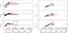 |
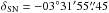
Fig. 4 Colour evolution of SN 2012aa and comparison with other events. All of the colours have been corrected for reddening. Left panel: four broad-lined SNe Ic (SNe 1998bw Clocchiatti et al. 2011; 2002ap, Foley et al. 2003; 2003jd Valenti et al. 2008a; and 2006aj Ferrero et al. 2006), along with the normal SN Ibc SN 2007uy (Roy et al. 2013) and two SLSNe Ic (SN 2007bi Young et al. 2010 and PTF12dam Nicholl et al. 2013) are compared with the colour evolution of SN 2012aa. The shaded region in the central panel ((V−R)0 colour) represents the colour evolution of SNe Ibc as discussed by Drout et al. (2011). Unlike normal and broad-lined SNe Ibc, SN 2012aa and SLSNe show evolution on longer timescales. Right panel: comparison with SLSNe (SNe 2012il, 2011ke, 2011kf, PTF 11hgi, and 11rks from Inserra et al. 2013; PTF 12dam from Nicholl et al. 2013; and SN 2010gx from Pastorello et al. 2010b). After maximum brightness, the colour of SNe Ibc appears to evolve quickly, whereas in SLSNe it evolves more slowly, becoming redder over a longer time. The sudden increment in the (B−V)0 (or (g−r)0) colour of SN 2012aa after +50 d is similar to the colour variation observed in SN 2010gx. |
4.3. Long-term photometry of the host galaxy
Figure 3 presents the long photometric monitoring of the host galaxy by CRTS, starting from ~2923 d before the discovery of SN 2012aa to + 515 d after discovery. The weighted mean magnitude of the host in V, indicated by the dotted line, is 19.11 ± 0.24; the long-dashed lines are 1σ and the short-dashed lines are 2σ limits. This value is consistent with the V-band measurement obtained years after the explosion (Sect. 2.1). The peak brightnesses of typical precursor events in massive stars varies roughly between − 10 and − 15 mag (Smith et al. 2010; Pastorello et al. 2010a; Smith et al. 2011). At the distance of SN 2012aa, this corresponds to an apparent brightness of ~22−25 mag, which is undetectable in the CRTS long-term monitoring.
In some of the very early-time (~2900 d) observations prior to the SN, we found that the measurements are marginally higher than the 2σ limit. Subtracting the mean flux of the host, this corresponds to a rise to ~20.75 mag, or ~− 17.59 mag on the absolute scale. This is about 3−7 mag more luminous than typical pre-SN outbursts of LBVs, and comparable only to the precursor activity of SN 1961V. If real, this early event caught by CRTS is more likely associated with some other SN that happened in the same host or is associated with nuclear activity in the host itself. However, we note that these early CRTS data were taken when the CSS-CCD system response was different10. This may also be why a higher flux is obtained for the object at early epochs.
5. Colour evolution and quasi-bolometric flux
Figure 4 presents the intrinsic colour evolution of SN 2012aa and a comparison with other SNe Ic and SLSNe. The left panel draws the comparison with SNe Ibc (e.g., SNe 1998bw, 2002ap, 2003jd, 2006aj, 2007uy) and Type I SLSNe (e.g., 2007bi, PTF12dam) in the Bessell system, while for better statistics a separate comparison between SN 2012aa and Type I SLSNe is shown in the right panel using Sloan colours. The Sloan colours of SN 2012aa have been calculated after converting Bessell magnitudes to Sloan magnitudes through “S-corrections” using the filter responses given by Ergon et al. (2014).
The difference in colours between SN 2012aa and other similar events (e.g., SN 2003jd, PTF12dam) at early epochs is below 0.5 mag. If we assume they have similar intrinsic colours, this confirms that our estimate of the line-of-sight extinction toward SN 2012aa is reasonable and thus establishes that SN 2012aa is indeed an intermediate-luminosity transient between CCSNe and SLSNe in terms of its peak absolute magnitude.
With a larger sample of SNe Ibc, Drout et al. (2011, see also the left panel of Fig. 4) found that the (V−Rc)0 colours of these SNe become redder (an effect of cooling; Piro & Nakar 2013; Taddia et al. 2015) within 5 d after explosion. Then they rapidly become bluer just before or around the peak (~20 d after explosion), and subsequently redder again starting 20 d post maximum. In contrast, the evolutionary timescale of SLSNe I is much longer. The (g−r)0, (r−i)0, and (r−z)0 colours evolve gradually from negative/zero values at around peak brightness to positive values (+0.5−+1 mag) by +50 d. Owing to a lack of data, both the early-time (before maximum brightness) and late-time (beyond +50 d) colour evolution of SLSNe is not well known. The few existing early-time and late-time observations of the Type I SLSNe 2011ke, 2011kf, and PTF12dam indicate that these SNe get bluer gradually well before their maxima, and keep roughly constant colour values beyond +50 d.
Since we do not have any multiband observations of SN 2012aa before peak, from the left panel of Fig. 4 it is difficult to assess whether this SN behaves like other CCSNe or not. Between +10 d and +50 d, the (B−V)0 colours of SN 2012aa are more similar to those of CCSNe than to those of the Type I SLSNe 2007bi and PTF12dam. The difference is negligible (and hence not conclusive) in (V−Rc)0 and (V−Ic)0 colours. A further comparison of SN 2012aa with a larger sample of SLSNe is presented in the right panel of Fig. 4. The increase in (g−r)0 of SN 2012aa is similar to that of SNe 2010gx, 2011ke, 2011kf, and PTF11rks. Like SN 2010gx, SN 2012aa also shows a jump in the (g−r)0 (and in (B−V)0) colour after +50 d, owing to a steeper decline in the blue filter.
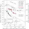 |
Fig. 5 BVRcIc quasi-bolometric light curve of SN 2012aa and other stripped-envelope CCSNe and SLSNe along with the luminous event SN 2010jl. The long dashed vertical line shows the epoch of V-band maximum light. The K-correction and cosmological time dilation effects have been taken into account. For the first two data points, we have only CRTS V-band data, while for the last four points there is incomplete coverage/detection in some bands. For these six epochs we have calculated the BVRcIc quasi-bolometric light curves after measuring the temporal evolution of (MBVRcIc−MV) as shown in the inset. |
The BVRcIc quasi-bolometric light curve has been constructed after accounting for the line-of-sight extinction, K-correction, and cosmological time dilation. A comparison of SN 2012aa with other SLSNe and CCSNe is presented in Fig. 5. The quasi-bolometric luminosities of SN 2012aa have been calculated for those epochs where the SN was detected in at least in two bands. For the epochs when SN was not observed in some band, the absolute magnitudes in corresponding bands were calculated by linear interpolation. It should be noted that for the first two epochs, we have only CRTS data, while for the last four points there is incomplete coverage/detections in all BVRcIc bands. For these six epochs we calculated the BVRcIc quasi-bolometric luminosities after measuring the temporal evolution of (MBVRcIc−MV) as shown in the inset of Fig. 5. Two different polynomials have been fitted to the dataset, calculated on the epochs for which MBVRcIc and MV were known. After excluding four deviant points we get the two following fits: for t< 50 d, (MBVRcIc−MV) = 0.0862−0.0018 t, while for t> 50 d, (MBVRcIc−MV) = −1.1125 + 0.0315 t−0.00016 t2, where t is the time elapsed after V-band maximum. The first fit was used to calculate MBVRcIc for the first two data points, while the second fit was used to calculate MBVRcIc for the last four epochs.
Fitting a third-order polynomial to the early part of the quasi-bolometric light curve sets the epoch of bolometric maximum about 7 d after V-band maximum, as mentioned in Sect. 4, or just 4 d after discovery. The rise and decline timescales for the quasi-bolometric light curve are respectively 34 d and 57 d, consistent with the corresponding values calculated from the V band (see Sect. 4.1).
In Fig. 5 we compare the BVRcIc quasi-bolometric light curve of SN 2012aa with those of SNe Ibc (e.g., SNe 1998bw, 2003jd, 2007uy) and the SLSN PTF12dam. For completeness, we also include the H-rich SLSNe 2006gy (Agnoletto et al. 2009) and CSS100217 (Drake et al. 2011), as well as the long-lived luminous transient Type IIn SN 2010jl (Zhang et al. 2012). It is clear that in terms of both peak luminosity and light-curve width, SN 2012aa is intermediate between SNe Ic and SLSNe I. It probably belongs to the class of luminous transients that are supported to some extent by an additional powering mechanism along with radioactive decay. In particular, the bumpy light curve strongly supports the CSM-interaction scenario. Between +60 d and +100 d after maximum brightness, the decline rate of the quasi-bolometric light of SN 2012aa is 0.02 mag d-1, steeper than the 56Co → 56Fe rate though consistent with the decline rates of SNe Ibc. Beyond +100 d the light curve of SN 2012aa became flatter.
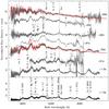 |
Fig. 6 Spectral evolution of SN 2012aa. All spectra were normalized to the average continuum flux density measured in the line-free region 6700−7000 Å and additive offsets were applied for clarity. The dotted vertical line shows the position of Hα. Phases are with respect to the date of maximum V-band light. The spectra obtained on +8 d and +51 d were modelled using SYNOW (red curves) to identify the important line features. |
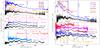 |
Fig. 7 Spectral comparison between SN 2012aa and other H-poor events. Phases are with respect to the date of maximum light. Left panel: similarities between SN 2012aa and the broad-lined Type Ic SNe 2003jd (Valenti et al. 2008a), 2006aj (Modjaz et al. 2014), and 2007gr (Valenti et al. 2008b), as well as the normal Type Ic SN 1994I (Modjaz et al. 2014), are shown. Spectra of SN 2012aa are similar, but redshifted relative to those of SN 2003jd. However, unlike the case for SN 2003jd, we can seeFe ii lines in SN 2012aa at early stages, quite similar to what was observed in SNe 1994I and 2007gr. Right panel: comparisons between SN 2012aa and Type Ic SLSNe (e.g., SN 2010gx, Pastorello et al. 2010b; SN 2007bi, Young et al. 2010; PTF12dam, SSS120810, Nicholl et al. 2013, 2014; and PTF09cnd, Quimby et al. 2011) are shown. The absence (or weakness) ofO ii andO iii lines in the early-time spectra of SN 2012aa distinguishes it from canonical Type Ic SLSNe. However, near +100 d, the spectra are similar to each other (except those of SN 2007bi), as shown in the lower half of this panel. |
6. Spectroscopic evolution of SN 2012aa
The upper panel of Fig. 6 presents the spectral evolution of SN 2012aa at seven phases, starting from +8 d to +113 d after maximum brightness. The spectra have been corrected for the redshift of the host galaxy (z = 0.083; see Sect. 3). In the lower panel, we show the +113 d spectrum once again with some important lines marked. The line identification is done mainly by comparing the spectra with previously published SN Ic and SLSN spectra having line identifications (Valenti et al. 2008a; Young et al. 2010; Nicholl et al. 2013). They are also based on models built using the fast and highly parameterized SN spectrum-synthesis code, SYNOW (Millard et al. 1999; Branch et al. 2002).
The position of narrow Hα is marked by a dotted vertical line. The narrow Hα in the +8, +22, +29, +91, and +113 d spectra is from the host galaxy. The separation between the SN and the galaxy center is ~1.96′′ (Sect. 7), comparable with the slit width. Thus, the detection of Hα is highly dependent on the slit orientation and seeing conditions on the night of observations. For example, in the observations on +47 d and +50 d, no host-galaxy line was found in the two-dimensional spectra of the SN. Similarly, the sharp spikes at ~5441 Å in the +22 d and +29 d rest-wavelength spectra are actually the footprints of telluric emission fromNa i D vapor (λλ5890, 5896) that was saturated during the observations. So, although the initial (<+50 d after maximum) spectra exhibit some relatively strong lines with weak broad components, which may resemble the electron-scattering effect during shock interaction, they are most likely emission lines from the host galaxy and/or unresolved telluric emissions in the low-resolution spectra.
6.1. Key features
The blackbody fit and SYNOW modelling of the spectra show that the blackbody temperature of the photosphere between +8 d and +113 d is between ~8000 K and 7000 K. The initial spectrum (+8 d) is dominated by a continuum with some broad lines. With time, the SN spectra become redder and the nebular lines start to appear. In Fig. 7, a comparison of the spectral evolution of SN 2012aa and that of SNe Ic and H-poor SLSNe is presented.
The initial spectrum (+8 d) of SN 2012aa is similar to (although redder than) that of the broad-lined Type Ic SNe 2003jd and 2006aj at − 2 d and − 5 d, respectively, relative to maximum brightness (see the top left panel in Fig. 7). We also compared the spectra of SN 2012aa taken at +8 d and +50 d after maximum with synthetic spectra generated with SYNOW. The spectra at late epochs are more emission-line dominated (because the ejecta became more optically thin), and SYNOW modelling becomes less useful. As shown in Fig. 6, most of the weak, broad lines in the bluer part of the +8 d spectrum are reproduced with broadFe ii (Gaussian FWHM ~ 14 000 km s-1); in addition, theCa ii H&K,Na i D, andCa ii λ8662 absorption dips are present. However, unlike broad-lined SNe Ic and more like normal SNe Ic (e.g., SNe 1994I and 2007gr), SN 2012aa starts to show narrower iron features much earlier after the epoch of maximum (Gaussian FWHM ofFe ii λλ4924, 5018, 5169 lines became ~5000 km s-1 by +22 d).
The noisy absorption feature at 6150 Å in the first spectrum can be reproduced either bySi ii at 12 500 km s-1 or by Hα at 20 000 km s-1, while the photospheric velocity is ~12 000 km s-1 (see Sect. 6.2). This feature can be blended withFe ii lines as well.
The +22 d and +50 d spectra of SN 2012aa are similar to the +26 d spectrum of SN 2003jd, with prominent features ofCa ii H&K,Fe ii blended withMg ii (and maybe withMg i ] λ4571 beyond +50 d), as well asCa ii ,O i , andO ii lines. By +47 d,Si ii absorption becomes more prominent. Finally, as shown in the bottom left panel of Fig. 7, unlike SNe 2012aa and 2003jd, beyond +100 d the normal SNe Ic (e.g., SNe 1994I and 2007gr) become optically thin, marked by the presence of strong nebular emission features of [O i ] λλ6300, 6364 and [Ca ii ].
In contrast to SN 2012aa, the spectra of Type I SLSNe near (or before) maximum exhibit an additional W-like absorption feature between 3500 and 4500 Å, which is the imprint ofO ii (Pastorello et al. 2010b; Quimby et al. 2011; Inserra et al. 2013). As shown in the right panel of Fig. 7, the early (+8 d) spectrum of SN 2012aa is redder than the +7 d spectrum of PTF12dam and the +10 d spectrum of SN 2010gx. The features in the blue part of the first spectrum of SN 2012aa are also not similar to those found in SN 2010gx and PTF12dam at comparable epochs. However, the late-epoch (~+ 113 d) spectrum of SN 2012aa is similar to that of SNe 2007bi, 2010gx, PTF09cnd, and PTF12dam.
Comparison of the spectral evolution of SN 2012aa with that of both SNe Ic and SLSNe suggests that the broad emission feature (Gaussian FWHM ≈ 14 000 km s-1) near Hα (marked “X” in the right panel of Fig. 7) could be the emergence of [O i ] λλ6300, 6364. It is prominent in the +47 d spectrum of SN 2012aa and marginally present already at +29 d. Although in comparison to other known events this feature is highly redshifted (~9500 km s-1 on +47 d) in SN 2012aa, a similar time-dependent redshift is also noticeable for other lines in SN 2012aa (see Sect. 6.3).
Alternatively, this feature could be blueshifted (1500−2500 km s-1) Hα emission that remains almost constant throughout its evolution. It becomes prominent by +47 d, contemporary with the peak of the secondary light-curve bump and consistent with the CSM-interaction scenario. Between +47 d and +113 d, the width (FWHM) of this feature remains at around 14 000 km s-1. The values of both the blueshift and FWHM would be higher than the corresponding values calculated for CSM-interaction powered SNe (see, e.g., Fransson et al. 2014). Moreover, we do not detect any other Balmer lines in the spectra, though it is also probable that they would be highly contaminated byFe ii and other metal lines, making them difficult to detect in low-resolution spectra.
It is noteworthy that a broad feature at similar rest wavelength was observed in a few other SLSNe (such as LSQ12dlf and SSS120810) during their early phases and identified as theSi ii λ6350 doublet (Nicholl et al. 2014; see also Fig. 7). However, unlike feature “X” (which was strong until +113 d), the feature in LSQ12dlf and SSS120810 was almost washed out by +60 d.
We next compare the blue part (3400−5600 Å) of the first spectrum of SN 2012aa with the early spectral evolution of SLSNe (e.g., SN 2010gx) and CCSNe (e.g., SNe 1994I, 2003jd, 2006aj; see Fig. 8). Although the broad features of SN 2012aa during this phase (such asCa ii ,Mg ii , andFe ii with Gaussian FWHM ≈ 12 000 km s-1) are similar to those in the +10 d spectrum of SN 2010gx, the early key features of SLSNe (likeO ii lines) are not detected in the spectra of SN 2012aa. The presence of theFe ii andMg ii blend (Gaussian FWHM ≈ 150 Å ) around 4800 Å in this early-time spectrum distinguishes it from canonical SLSNe and broad-lined CCSNe (like SNe 2003jd and 2006aj). At comparable epochs, both SLSNe and broad-lined SN Ic spectra show a very broad absorption dip (FWHM ≈ 350 Å in SN 2010gx), which is probably a blend ofFe ii multiplets. On the other hand, the Type Ic SNe 1994I and 2007gr exhibitFe ii andMg ii blends that are quite similar to those of SN 2012aa.
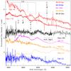 |
Fig. 8 Blue part (3400−5600 Å) of the early-time spectra of SN 2012aa and comparison with other SNe Ic and H-poor SLSNe. It is difficult to determine whether SN 2012aa belongs to the SLSN or the CCSN category. |
Furthermore, in terms of the timescales, the features that distinguish SN 2012aa from SLSNe are visible in the red part (>7000 Å) of the spectra. The lines [Ca ii ] λλ7291, 7324, [O ii ] λλ7319, 7330,O i λ7774,Ca ii λλ8498, 8542, 8662, and [C i ] λ8730, which are strong in SN 2012aa spectra starting from +50 d, are barely detected before +80 d in the SLSN samples presented by Inserra et al. (2013). Although theO i andCa ii near-infrared lines start appearing beyond +50 d in SLSNe, Nicholl et al. (2015) also noticed that these features (along with other forbidden lines like [Ca ii ]) become strong only at ≳+ 100 d after maximum. These lines are instead common in SNe Ibc, even just after maximum brightness (e.g., Millard et al. 1999; Branch et al. 2002; Valenti et al. 2008a; Roy et al. 2013), and also in SNe II during the late photospheric phase (Filippenko et al. 1994; Pastorello et al. 2004). In this sense, SN 2012aa is more similar to SNe Ic than to Type I SLSNe.
To summarize, although the overall spectral evolution of Type I SLSNe is similar to that of canonical SNe Ic, the timescales for SLSNe are much longer than for their corresponding low-luminosity versions. The nature of the SN 2012aa light curve is more similar to that of SLSNe, while the timescale (and nature) of its spectral evolution more closely resembles that of normal SNe Ic.
However, there are caveats. The Type I SLSNe like PTF11rks started to exhibitFe ii ,Mg ii , andSi ii features from ~+ 3 d post maximum, as is common in SNe Ic. Beyond +60 d the distinctFe ii multiplet features near 5000 Å were noticed in SLSN PTF11hgi (Inserra et al. 2013; Nicholl et al. 2015). These were not prominent in the broad-lined SNe Ic associated with engine-driven explosions such as SNe 1998bw, 2006aj, 2003dh, 2003jd, and 2003lw at comparable epochs, although present in the Type Ic SNe 1994I and 2007gr, and also in stripped-envelope SNe Ib like SN 2009jf (Valenti et al. 2011). It is also worth noting that the emission lines in SN 2012aa start appearing at a relatively early stage in comparison to what is seen for SLSNe, and there is no considerable change in the features beyond +50 d. Almost all features persist up to the epoch of the last (+113 d) spectrum with comparable line ratios, which is unusual in normal SNe Ic. In that sense, the timescale of SN 2012aa is longer than that of most normal SNe Ic.
6.2. Photospheric velocity
TheFe ii λλ4924, 5018, 5169 absorption lines throughout the spectral evolution helped us determine the photospheric velocity (vphot) of SN 2012aa. Figure 9 illustrates a comparison of the velocities of these metal lines in SN 2012aa with the photospheric velocities of other SNe Ic and SLSNe. Uncertainties are calculated by estimating the scatter in repeated measurement of the absorption dips; the error bars represent the 2σ variation. Although near peak brightness the velocities of individual lines are comparable with each other; at late stages a deviation in their velocities is noticed. The dashed line represents the average velocities of these three lines and can be considered as representative of the photospheric velocity of SN 2012aa.
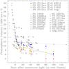 |
Fig. 9 Comparison of the photospheric velocity of SN 2012aa with that of SNe Ibc and SLSNe. Velocities ofFe ii λλ4924, 5018, 5169 absorption in SN 2012aa are indicated with filled squares, circles, and triangles, respectively. The dashed line represents the average photospheric velocity of SN 2012aa calculated from theFe ii lines. All of the transients labelled in the left column are SNe Ibc, while the SLSNe Ic are labelled in the right column. For all SLSNe, the velocities at individual epochs have been connected with dotted lines. The photospheric velocities (measured fromFe ii andSi ii lines) of other transients in the plot have been adopted from the literature: SN 2007bi from Young et al. (2010); all other SLSNe are from Nicholl et al. (2015); SNe 2002ap, 2006aj, and 2008D are from Mazzali et al. (2008); SNe 1994I and 1998bw are from Patat et al. (2001); SNe 2003jd, 2007gr, and PTF10qts are from Valenti et al. (2008a), Hunter et al. (2009), and Walker et al. (2014), respectively. |
The average evolution of these Fe lines sets vphot to ~11 400 km s-1 at maximum brightness. The comparison (Fig. 9) shows the SN 2012aa velocity evolution is comparable to that of SNe Ibc rather than to the shallow velocity profiles of SLSNe. The flattened velocity profiles of SLSNe and in contrast to that for CCSNe has been seen in moderate samples (~15 objects, Chomiuk et al. 2011; Nicholl et al. 2015; see also Fig. 9). Such a velocity evolution in SLSNe had been predicted as a consequence of the magnetar-driven explosion model; if the energy released by the spin-down magnetar is higher than the kinetic energy of the SN, the entire ejecta will be swept up in a dense shell and will propagate with a uniform velocity until the shell becomes optically thin to electron scattering on a timescale of 100 d after explosion (Kasen & Bildsten 2010). On the other hand, a power-law decline of the photospheric velocities in SNe Ibc is a consequence of homologous expansion. Since the average photospheric velocity profile of SN 2012aa is similar to that of CCSNe, a homologous expansion is more likely in SN 2012aa than a magnetar-driven scenario.
6.3. Line velocities
Figure 10 shows the velocity evolution of different lines at around 4571 Å, 5893 Å, 6300 Å, and 7774 Å. The zero velocity of each panel corresponds to the above-mentioned rest wavelengths (marked at the top of each panel).
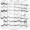 |
Fig. 10 Temporal evolution of some spectral windows in SN 2012aa. The zero velocity shown with a dotted line in each panel marks the rest wavelength of the corresponding element mentioned at the top of the panels. The flux density scale is relative. The flux of each line has been scaled in the same way as for the entire spectra mentioned in Fig. 6. The dashed lines are the boundaries between which the emission peaks and absorption dips get shifted during the SN evolution. The downward arrows in the second panel show the blueshift of theNa i D absorption. The arrow marked with “X” shows the emergence of [O i ] by +29 d. |
If the SN emission is not shock-dominated, the spherical homologous expansion of optically thick ejecta would produce a spectrum with simple P-Cygni line profiles that are a combination of emission and absorption features; the emission peak is always centered at the rest wavelength of the line (and hence at zero velocity in the rest frame), while the absorption dip gets blueshifted, which is a measure of outflow velocity. Unlike this simple P-Cygni feature, we noticed a velocity evolution of the emission components of several spectral lines in SN 2012aa. As shown in Fig. 10, near maximum light the emission feature near 4571 Å (tentatively marked as a blend ofFe ii andMg ii ) was blueshifted from the rest position by − 5000 km s-1. With time this feature became redshifted by 10 000 km s-1, and finally at +113 d it was redder with a projected velocity of ~+5000 km s-1. Similarly, after its emergence at around +29 d, the [O i ] λλ6300, 6364 doublet (marked by the “X” in the third panel) also exhibits a redshift of 10 000 km s-1, consistent with the redshift of the emission feature at 4571 Å. Similar velocity evolution of the emission lines could indicate an aspherical evolution of these line-forming regions. This kind of analysis depends on the assumption that we can identify single elements that dominate the time evolution of their spectral region. The redshift of the feature near 4571 Å may be caused by the emergence of theMg i ] emission line. However, in SNe Ibc at comparable epochs (≳110 d post maximum) the strength of this semi-forbidden line is often much less than that of other nebular lines (e.g., Taubenberger et al. 2009, their Fig. 1). In SN 2012aa at similar epochs this feature is stronger than that observed in SNe Ibc. Moreover, ~5000 km s-1 redshift with respect to its rest position at this stage (+113 d) of evolution makes this line quite unlikely to beMg i ] in a spherically expanding SN envelope.
The absorption dip of theFe ii plusMg ii blend is at ~− 18 200 km s-1 in the first spectrum, while in the last spectrum it is at ~− 13 200 km s-1. Similarly, the FWHM of [O i ] at +47 d is ~11 900 km s-1, and it decreased to ~9700 km s-1 by +113 d. Similarly, the absorption dip of theNa i D line is at ~13 000 km s-1 at +22 d and decreased to ~10 500 km s-1 by +113 d post maximum. Such values are higher than the photospheric velocity (Sect. 6.2), indicating that these line-emitting regions could be detached from the photosphere.
The shapes of line profiles of Fe-group elements and [O i ] are dependent on the distribution of 56Ni inside the ejecta and/or can be affected by blending (even for a symmetric distribution of 56Ni). Even with an extremely aspherical distribution of 56Ni inside spherical ejecta, the [O i ] profile can be distorted by ~3000 km s-1 (Maeda et al. 2008; Modjaz et al. 2008b). Thus, the highly redshifted lines in SN 2012aa probably indicate an extreme asphericity in the ejecta themselves, perhaps the ejection of a blob receding at ~10 000 km s-1.
TheO i λ7774 line, which started to emerge almost simultaneously with [O i ] λλ6300, 6364 (see fourth panel of Fig. 10), evolved like a canonical P-Cygni feature: the emission peak remained at around zero velocity, while the absorption dip was initially blueshifted by ~− 10 000 km s-1, slowed down, and finally stayed at ~− 5000 km s-1. This suggests a spherical homologous expansion of this particular line-emitting region and contrasts with the evolution of the “X” profile, if we assume it to be [O i ] λλ6300, 6364. We speculate that this situation can only happen under extreme asymmetry, when a blob enriched with [O i ] λλ6300, 6364 is ejected away from the expanding SN with a velocity of ~10 000 km s-1.
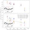 |
Fig. 11 Velocity evolution ofFe ii lines in SN 2012aa. The three linesFe ii λλ4924, 5018, 5169 are difficult to identify unambiguously. We found two different possibilities in SN 2012aa, shown here using the +50 d spectrum; the lines are respectively marked with blue, orange, and red arrows in the insets. Lower panel: the velocity evolution is a power law common in CCSNe. Upper panel: the velocity evolution has a shallow decline common in SLSNe. |
6.4. Fe II velocities
In Fig. 11, we show the +50 d spectrum of SN 2012aa, marking three absorption lines ofFe ii λ4924, λ5018, and λ5169 in blue, orange, and red, respectively. The lower panel illustrates that in one set of combinations theFe ii velocity profile is close to a power law, representing homologous expansion, and is comparable to the photospheric velocity profiles of CCSNe. This velocity is consistent with the profile of other elements, and we therefore consider it to be the representation of the photospheric velocity of SN 2012aa (used in Sects. 6.2 and 6.3). On the other hand, if we used a different set of absorption-line combinations (shown in the upper panel of the figure), we would get a shallow velocity profile more consistent with that of SLSNe (see Fig. 9).
Although the power-law profile is more feasible in SN 2012aa, the shallow decline cannot be completely ruled out. In this case the velocity profiles of individualFe ii lines are actually more mutually consistent, and in all SYNOW models we get a better fit forFe ii lines by keeping their velocities higher than the photospheric velocity, and evolving them as a detached shell. From the spectrum (Fig. 11, upper panel) we can also see that Gaussian FWHM values (~3000 km s-1) of theFe ii lines in this combination are more consistent with each other than the alternative combination (lower panel). If the shallow profile (upper panel) were maintained by theFe ii in SN 2012aa, along with a lower photospheric velocity profile (like in the lower panel), we would be able to draw the following conclusions.
The velocity ofFe ii lines at maximum brightness is ~18 000 km s-1, declines to ~16 000 km s-1 within 20 days, and remains constant at that value for the next 60 days, finally dropping to 12 000 km s-1 at 100 d after the peak. In this scenario, the velocity profile ofFe ii lines in SN 2012aa is much higher than the typical velocities of SLSNe (e.g., 10 500 ± 3100 km s-1; Nicholl et al. 2015) measured at a comparable phase. Higher bulk velocity along with a narrow velocity spread (FWHM) ofFe ii absorption lines is not common among SNe Ic; high velocities of the lines generally make the corresponding profiles broader (Modjaz et al. 2015).
7. Properties of the host galaxy
The spectral and photometric differences of SN 2012aa compared with the well-known canonical CCSNe and Type I SLSNe motivate us to investigate the nature of its host.
Figure 12 presents the spectrum of the host taken ~905 d after the SN discovery, when the SN had disappeared. It exhibits the Hα line along with [N ii ] λλ6548, 6584, [S ii ] λλ6716, 6731, Hβ, and [O ii ] λ3727, characteristic of a spiral galaxy with Sa/Sb/Sbc subclasses (Kennicutt 1992). Fixing the morphological index (T-type) parameter for this galaxy as 3.3 from the “Third Reference Catalog (RC3) of Bright Galaxies” (de Vaucouleurs et al. 1991) and assuming (from optical images) a position angle of ~0°, we calculate a typical deprojected dimension of the host as ~6′′, corresponding to a physical size of ~8 kpc. Thus, the host of SN 2012aa is much smaller than our own Milky Way Galaxy and other spiral hosts of nearby SNe Ibc.
Measurements of the overall metallicity of the host and that at the SN location are important for understanding the properties of the birth places of SN progenitors. The first entity can be measured either in an indirect way from the B-band luminosity of the host (Tremonti et al. 2004) or directly after calculating the [N ii ] λ6584/Hα ratio in the host nucleus (Pettini & Pagel 2004). These diagnostics have been used by several similar studies (e.g., Anderson et al. 2010; Taddia et al. 2013, and references therein).
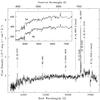 |
Fig. 12 Optical spectrum of the host-galaxy center taken with NOT +905 d after discovery of SN 2012aa. Prominent lines are marked. The spectrum suggests that the host is a typical star-forming galaxy of Type Sa/Sb/Sbc. From the observed wavelength of Hα, we measured the host-galaxy redshift to be z = 0.083. |
The apparent B magnitude of the host is 20.17 ± 0.06, which corresponds to an absolute magnitude of ~− 18.13. Using the empirical relationship between B-band luminosity and metallicity found for SDSS galaxies (Tremonti et al. 2004), we find the overall metallicity of the host to be [12 + log(O/H)]  dex. This implies the overall metallicity of the host, Z ≈ 0.78 Z⊙, where [12 + log(O/H)]⊙ ≈ 8.69 dex is the solar metallicity in terms of oxygen abundance (Asplund et al. 2009).
The second method is to calculate the metallicity from the [N ii ] λ6584/Hα ratio, the so-called N2 diagnostic (Pettini & Pagel 2004). Owing to the similar wavelengths of these lines, this method is neither dependent on the correct measurement of extinction nor affected by differential slit losses. From our +905 d spectrum, we measure this flux ratio to be 0.391, which gives the metallicity of the host of [12 + log (O/H)] ≈ 8.72 dex, which corresponds to Z ≈ 1.07 Z⊙.
Hence, the overall metallicity of the host is Zhost = 0.92 ± 0.34 Z⊙, which is consistent both with the solar metallicity and with the average metallicity of the star-forming galaxies hosting SNe IIP and normal SNe Ibc (Anderson et al. 2010).
The diagnostic tool known as a BPT diagram (Baldwin et al. 1981) is an important means for determining the nature of the host. It shows the distribution of galaxies in the log([N ii ]/Hα) vs. log([O iii ]/Hβ) plane. Different schemes have been proposed to classify the galaxies using SDSS data (e.g., Kewley et al. 2006). Using this tool, it has been found that SLSNe generally reside in galaxies that are considerably different from star-forming galaxies hosting CCSNe (see Sect. 9). We use the BPT diagram to diagnose the host of SN 2012aa. We measure log ([N ii ]/Hα) =−0.407, but [O iii ] emission is absent in the host spectrum. Considering the continuum flux level as the minimum possible flux of [O iii ] we find log([O iii ]/Hβ) ≲−0.796. These two quantities satisfy the inequality (see Kewley et al. 2006) log ([O iii ]/Hβ) < 0.61/[log ([N ii ]/Hα) − 0.05] + 1.3, which defines the region of star-forming galaxies in the BPT diagram. Thus, we conclude that the host of SN 2012aa is a normal star-forming galaxy. This is consistent with the conclusion drawn from the metallicity measurement.
8. Physical parameters
The SN can be powered either entirely by radioactive 56Ni →56Co decay or by CSM interaction (or both). Here we discuss the two scenarios for SN 2012aa.
8.1. Radioactive powering
We adopt the analytical relations of Arnett (1982) to estimate explosion parameters from the observables. Assuming the power source to be concentrated in the inner parts of the ejecta, the total ejected mass (Mej) and the amount of 56Ni produced during explosive nucleosynthesis can be derived from both the peak and tail luminosities of SN 2012aa. It can also be measured by fitting the light curve of SN 2012aa with the stretched and scaled light curve of SN 1998bw, for which the Ni mass and Mej are known (Cano 2013).
The BVRcIc quasi-bolometric light curve of SN 2012aa shows a declining tail with a rate of 0.02 mag d-1 from +60 d to +100 d. This is comparable to the decline rates of SNe Ibc (see Sect. 4.2). Under the assumption that for SN 2012aa this phase is mainly powered by radioactivity, the scaling relation to SN 1987A can be applied to estimate the amount of 56Ni. Assuming the rise time of SN 2012aa is ≳30 d, we can say that the luminosity of SN 2012aa is (L12aa)130 ≈ 2.4 × 1042 erg s-1 roughly 130 d after explosion. At a comparable phase, the BVRcIc luminosity of the well-studied Type II SN 1987A was (L87A)130 ≈ 1.2 × 1041 erg s-1. Assuming that in both events the γ rays from radioactive yields were fully trapped inside the ejecta at 130 d after the explosion, we can write (L12aa)130/ (L87A)130 ≈ (MNi)12aa/ (MNi)87A, and under the above-mentioned assumption we obtain a lower limit of the amount of radioactive Ni for SN 2012aa, (MNi)12aa ≈ 1.4 M⊙, where (MNi)87A = 0.075 M⊙ (Elmhamdi et al. 2003).
Following Arnett (1982), the amount of 56Ni can also be calculated from the peak luminosity after accounting for the peak width of the light curve, which is an estimate of the diffusion timescale. Using the same analytical approach, and taking only the rise time into account, Stritzinger & Leibundgut (2005) found the following relation for Type I events:
![\begin{eqnarray*} && M_{\rm Ni}/{{M}_\odot} = (L_{\rm peak}/{\rm erg}\,{\rm s}^{-1})/\\ &&\left[6.45\times10^{43}\,{\rm e}^{-t_r/8.8} + 1.45\times10^{43}\,{\rm e}^{-t_r/111.3}\right], \end{eqnarray*}](/articles/aa/full_html/2016/12/aa27947-15/aa27947-15-eq219.png) where tr is the rise time in days, MNi is in solar mass units, and Lpeak is the peak luminosity in erg s-1. However, this expression is more applicable for those cases where the rise time is comparable to the decline time and hence the diffusion timescale can be quantified only by tr. For different rise and decline times, tr can be replaced by the geometric mean (τm) of τris and τdec. For the quasi-bolometric curves, for SN 2012aa we get τm ≈ 44 d. Since Lpeak ≈ 1.6 × 1043 erg s-1, this implies MNi ≈ 1.6 M⊙, consistent with the value found from the late-time light curve.
where tr is the rise time in days, MNi is in solar mass units, and Lpeak is the peak luminosity in erg s-1. However, this expression is more applicable for those cases where the rise time is comparable to the decline time and hence the diffusion timescale can be quantified only by tr. For different rise and decline times, tr can be replaced by the geometric mean (τm) of τris and τdec. For the quasi-bolometric curves, for SN 2012aa we get τm ≈ 44 d. Since Lpeak ≈ 1.6 × 1043 erg s-1, this implies MNi ≈ 1.6 M⊙, consistent with the value found from the late-time light curve.
Moreover, considering both diffusion timescale and velocity at the peak, the amount of ejected mass can be derived (Arnett 1996; Nicholl et al. 2015) as  where vphot is the peak photospheric velocity in cm s-1 and k is the opacity. In the literature different values of k have been adopted, normally varying between 0.05 and 0.1. To maintain consistency with the approach of Cano (2013), we adopt k = 0.07 cm2 g-1. For τm ≈ 44 days and vphot = 11,400 kms, we then get Mej ≈ 24 M⊙.
Here it is important to note that this is the maximum possible amount of 56Ni produced by SN 2012aa if and only if the entire light curve is powered by radioactivity. Although the amount of 56Ni derived from the tail luminosity and peak luminosity are consistent with each other, the secondary peak in the light curve makes this scenario unlikely. The data during the late phases does not allow us to constrain the onset of the optically thin phase powered only by radioactive decay. If we consider that intrinsically the SN 2012aa light curve is symmetric around the radioactively powered peak while the slow decline is instead produced by CSM interaction, we can replace τm by τris = 34 d in the two above expressions and get Mej ≈ 14 M⊙ and MNi ≈ 1.3 M⊙.
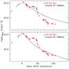 |
Fig. 13 BVRcIc quasi-bolometric light curve of SN 1998bw is fitted to that of SN 2012aa by stretching and scaling. Lower panel: for this fit the data points of SN 2012aa during its secondary bump have not been considered. Upper panel: for this fit the data points during the secondary bump have been considered. See text for details. |
In another approach (Cano 2013), we also use the BVRcIc quasi-bolometric light curve of SN 1998bw published by Clocchiatti et al. (2011) as a template and fit it to that of SN 2012aa by stretching along the time axis and scaling in luminosity (see Fig. 13). In the lower panel we have not considered the data points of SN 2012aa observed during the secondary peak, giving Mej = 10.9−11.7 M⊙ and MNi = 1.3−1.4 M⊙. These results are consistent with the values obtained from Arnett’s rule considering only τris. However, as shown in Fig. 13, this process cannot fit the very first observation. We also fit the peak of the light curve considering also the bump (upper panel, Fig. 13). Obviously, it will not fit the late part, but it can describe the rise well. The obtained values for this fit are Mej = 28.4−30.0 M⊙ and MNi = 1.2−1.3 M⊙. These values are reasonably consistent with results obtained by considering the higher velocity profile ofFe ii lines with peak vphot = 18 000 km s-1 and τris = 34 d: Mej = 22.9 M⊙ and MNi = 1.3 M⊙.
For the rest of this work, after comparing the spectroscopic and photometric properties of SN 2012aa with those of other CCSNe and SLSNe, we have adopted the following approximate values for the ejected mass and amount of 56Ni produced by SN 2012aa: Mej ≳ 14 M⊙ and MNi ≈ 1.3 M⊙. Hence, the kinetic energy of the explosion (Arnett 1996) is roughly EK = 0.3 Mejvphot2 ≈ 5.4 × 1051 erg.
8.2. CSM interaction powering
The presence of a secondary bump in the light curves implies that radioactivity is not the only power source for SN 2012aa. Another way to obtain such high luminosity is CSM interaction. For strong CSM interaction, a dense environment is required. Comparing the rise and decline timescales of SN 2012aa with those of other interacting SLSNe and SNe Ic (Nicholl et al. 2015, and references therein), suggests that ~5−10 M⊙ of CSM was expelled by the progenitor, while the amount of ejected mass could be ~10−15 M⊙.
We compare our light curves with results from recent hydrodynamical simulations from Sorokina et al. (2016), where the importance of CSM interaction in SLSNe was investigated. According to this study, an optical light curve with a sharp rise (~20 d) before peak along with a fast decline after +50 d is possible in an explosion with ejected mass of only 0.2 M⊙ and kinetic energy ~2 × 1051 erg within a 9.7 M⊙ CSM having a wind profile with index ~1.8. On the other hand, a longer rise time (~50 d) and shallow decline in the optical post-peak light curve was achieved by an explosion with ejected mass 5 M⊙ and kinetic energy ~4 × 1051 erg within a 49 M⊙ CSM.
The light-curve properties of SN 2012aa fall between these two categories. Fine tuning of the parameters could likely get a better match for the pure CSM interaction scenario, but we also note that the simulations of Sorokina et al. (2016) do not include the effects of 56Ni, which could be an oversimplification, and that the existence of a secondary bump requires the CSM to be distributed in a dense shell rather than in a constant wind. SN 2012aa could be an example where a combination of both radioactive decay and CSM interaction is responsible for the light-curve evolution.
8.3. Magnetar powering
A third scenario is the presence of a central engine, a proto-magnetar releasing spin energy that eventually powers the light curve over a long time. Several SLSN bolometric light curves have been modelled using this prescription. Here we have adopted the semi-analytical model developed by Inserra et al. (2013). We assumed that the secondary bump in SN 2012aa is produced by some other physical process; hence, when modelling we do not try to fit the data obtained during that period.We assumed that the photospheric velocity during the principal peak is ~12 000 km s-1, the kinetic energy of the explosion is ~1051 erg, and the rise time is 30−35 d. The best-fit model obtained by following Levenberg-Marquardt (LM) least-squares minimization technique (Moré 1978) is shown in the upper panel of Fig. 14, while the lower panel shows the residual. It gives the following values for the explosion parameters: Mej = 16.0 ± 1.7 M⊙, magnetic field of the proto-magnetar B = (6.5 ± 0.3) × 1014 G, and initial spin period P = 7.1 ± 0.6 ms. Apart from the bump, the model describes the overall broad observed light curve of SN 2012aa. The model deviates slightly (within the errors, however) from the observed light curve beyond +60 d past maximum.
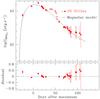 |
Fig. 14 Fitting the magnetar model to the observed BVRcIc quasi-bolometric light curve of SN 2012aa. We adopted the model proposed by Inserra et al. (2013). However, we only consider the power supplied by the magnetar, not that of radioactive decay. The errors associated with the observations have been calculated after propageting the errors in magnitudes only. While getting the best-fit model we have excluded the data that corresponds to the bump in the light curve (marked by the open circles). The Residual of the best-fit model has been shown in the lower panel along with the fitted data points (filled circles). Here Residual is defined as: Residual = (Observeddata−Modeldata) /Modeldata. For the best-fit model we found Mej = 16.0 ± 1.7 M⊙, the magnetic field of the proto-magnetar B = (6.5 ± 0.3) × 1014 G, and the initial spin period P = 7.1 ± 0.6 ms. |
9. Discussion in the context of other events
From the above analysis it seems that SN 2012aa is an intermediate object between normal SNe Ic and SLSNe I. In this section we discuss the optical characteristics of SN 2012aa in the context of SNe Ic and SLSNe.
9.1. Comparison of photometric characteristics
The Rc-band absolute magnitude at peak (MR ≈ −20 mag) of SN 2012aa is on the bright end, though consistent with that of the SN Ic distribution (− 19.0 ± 1.1 mag; Drout et al. 2011). However, its broader peak and higher tail luminosity require a larger amount of radioactive 56Ni and more ejected mass if modelled with the Arnett law. In addition, the presence of the secondary bump in the light curve requires some additional physical process.
As shown in Fig. 5, the peak bolometric luminosity of SN 2012aa is ~1.6 × 1043 erg s-1 (MBVRcIc ≈ −19.9 mag), which is higher than that of engine-driven explosions such as the Type Ic SNe 1998bw (~7.5 × 1042 erg s-1), 2006aj (~5.9 × 1042 erg s-1), 2003jd (~6.5 × 1042 erg s-1), and the normal Type Ib SN 2007uy (~6.4 × 1042 erg s-1). However, it is much less than the average peak luminosity (~8.2 × 1043 erg s-1 or MBol ≈ −21.7 mag) of Type I SLSNe (Quimby et al. 2013) and of slowly declining SLSNe exemplified by PTF12dam (Nicholl et al. 2013) in Fig. 5. In SLSN-I the typical decline rates after maximum brightness are much faster than the radioactive decay rate of 56Co. For example, in SN 2010gx the g, r, and i decline rates were γg ≈ 0.135, γr ≈ 0.084, and γi ≈ 0.086 mag d-1. Similar measurements for SNe Ibn like SN 2011hw give γB ≈ 0.058, γV ≈ 0.052, γR ≈ 0.055, and γI ≈ 0.047 mag d-1. It was argured that the steeper decline than radioactive decay in these SNe is due to powering by CSM interaction with no 56Ni or it is caused by substantial dust formation at late epochs (Pastorello et al. 2010b, 2015). On the other hand, in the slowly declining SLSNe (e.g., PTF12dam) or SLSN-R (e.g., SN 2007bi) the decline rate is much slower: for PTF12dam the values are γg ≈ 0.02, γr ≈ 0.014, and γi ≈ 0.015 mag d-1, while for SN 2007bi the values are γB ≈ 0.024, γV ≈ 0.018, γR ≈ 0.012, and γI ≈ 0.006 mag d-1. These values are comparable (but not identical) to 56Co decay.
By studying the evolution of bolometric light curves of SLSNe, Nicholl et al. (2015) found that for H-poor SLSNe-I, 20 ≲ τdec ≲ 40 d (i.e., 0.05 >Rdec> 0.03 mag d-1), while for SLSN-R τdec ~ 55−90 d (i.e., 0.02 >Rdec> 0.01 mag d-1). The rise timescales of these two sets of SNe are respectively 10 ≲ τris ≲ 25 d and 25 ≲ τris ≲ 40 d. They also found that for the entire sample τdec>τris, and generally τdec increases with τris, implying two possible distributions of SLSNe in the τris vs. τdec plane, where one set of SLSNe (with smaller values of τris and τdec) falls near the position of normal CCSNe.
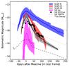 |
Fig. 15 Comparison of the SN 2012aa quasi-bolometric light curve with those of SLSNe Ic and SNe Ibc. The SLSN datasets are obtained from Inserra et al. (2013) and Nicholl et al. (2015), while the SN Ibc datasets are from Taddia et al. (2015). SLSN-R are distinctly different from SLSN-I. There may be two categories (A and B) of SLSN-I. The solid lines represent the mean of each population. The plot also presents the decay rate of 56Co and the well-observed Type II SN 1987A, which had a nebular decline consistent with 56Co decay. |
The rise and decline timescales of the bolometric light curve of SN 2012aa are τris = 34 d and τdec = 57 d, which implies that this SN is an event that falls between the two aforementioned distributions. Its decline (~0.03 mag d-1) before the secondary bump is similar to that of SLSN-I and SNe Ic, while the relatively slower decline (0.02 mag d-1) after +70 d is similar to SLSN-R and is not very different from that expected from 56Co decay. We also note that among the SLSNe-I (which behave similar to SNe Ic in the τris vs. τdec plane), some events (e.g., SNe 2011ke, 2012il, PTF10hgi, LSQ14mo; see Nicholl et al. 2015, their Fig. 1) show a decline trend after ~60 d past maximum that is similar to SN 2012aa (i.e., 0.02 mag d-1) and comparable to 56Co decay.
Figure 15 presents the light curves of different SNe Ibc and SLSNe I along with that of SN 2012aa11 as well as the Type II SN 1987A which has a late-time decline consistent with 56Co decay. Some SLSNe I start to show flattening in their light curves at earlier phases than others in this group. Before +60 d, they decline faster (≳0.03 mag d-1), while at later stages the slope is more shallow (~0.02 mag d-1). It seems that the events PTF10hgi, SN 2011ke, SN 2012aa, and SN 2012il belong to a subset that exhibits the photometric characteristics of both SLSNe-I (potentially shock dominated) and SLSNe-R (potentially radioactivity dominated).
Based on Fig. 15, we tentatively divide SLSN I into two categories (hereafter A and B). The SNe that fall inside the first set (category A) decline faster than the decay rate of 56Co, while the events that fall in the second set (category B) may show a radioactive decay phase (≳60 d after maximum light). At a considerable time after maximum (e.g., at +150 d as shown in figure), the second set becomes brighter than the first set, although dimmer than SLSNe-R. We also note that the mean peak width (measurement of the diffusion timescale) of category B is narrower than for category A. More extensive follow-up observations of these events at late phases are required to further understand any different subclasses of these stellar explosions.
9.2. Comparison of host properties
Using a sample of 23 SLSN hosts, Leloudas et al. (2015) found that H-poor SLSNe mostly occur in extreme emission-line galaxies (EELGs; Amorín et al. 2015), whereas SLSNe-II can be found in more massive, metal-rich, and relatively evolved galaxies. In contrast to H-poor SLSNe, broad-lined SNe Ic have not been found in EELGs and are associated with evolved star-forming galaxies (Modjaz et al. 2008a). In this context the host of SN 2012aa provides an example, with MB ≈ −18.13 mag and Zhost = 0.92 ± 0.34 Z⊙. This means that it is between the ordinary star-forming galaxies and the hosts of GRB-associated events, where the latter preferentially occur in low-luminosity and low-metallicity environments (Modjaz et al. 2008a).
With an extended galaxy sample, Anderson & Soto (2013) found that the hosts where only a single CCSN has been found have a median absolute magnitude as low as − 20.64 in B (see also Taddia et al. 2013, for the cumulative distribution of the B magnitudes of the host galaxies of CCSNe). The host of SN 2012aa has absolute B magnitude ~− 18.13. This implies that SN 2012aa occurred in a fainter galaxy than those that normally host CCSNe.
9.3. Investigating other possibilities
There are other scenarios which may produce a light curve and/or spectra similar to those observed in SN 2012aa.
As discussed in Sect. 1, TDEs also fill the luminosity and timescale gap between CCSNe and SLSNe. However, these events are generally expected to occur in galactic nuclei where the supermassive black hole (SMBH) resides. They could potentially be found at a location away from the center, if the entire system has two SMBHs. SN 2012aa exploded in the outskirts of its host, and in the late-time template image taken with the TNG we do not see any additional flux enhancement at the SN location. There is thus no evidence for a SMBH at the location of the SN. The spectral behaviour of SN 2012aa is also not comparable with those of known TDEs.
If the emission near Hα is indeed due to H, it could be preferable to call SN 2012aa a Type II event. Several SNe IIn and Ibn have been discovered with peak magnitudes between ~− 19 and − 20 (Zhang et al. 2012; Pastorello et al. 2016, and references therein). In all such cases, strong, narrow emission features (from unshocked CSM) with a broad component (from shocked CSM, predominantly H and/or He) have been observed. This was not seen in SN 2012aa. The impression of a narrow Hα line in the first three spectra is instead most likely caused by contamination by emission from the host center, which was unresolved from the SN during the observations. Spectral comparison with other events shows that SN 2012aa is of Type Ic. The colour evolution of SN 2012aa is also more similar to that of SNe Ibc rather than to SNe IIn, where a monotonic increase of colour with time is usually observed (Zhang et al. 2012).
As discussed in Sect. 1, the Type Ibc SN 2005bf and a few SLSNe I also showed double peaks in their light curves. In contrast, SN 2012aa exhibited a short-duration peak after the principal broader peak. In the relativistic jet or high-pressure bubble explosion scenarios, the short-duration bump is expected to occur before the broader peak (because of the shorter dynamical timescale). We can therefore rule out these two mechanisms for the formation of the secondary bump in SN 2012aa. Nevertheless, the presence of a spin-down magnetar as a central source of energy cannot be ruled out; the broader peak of SN 2012aa could be powered by a spin-down magnetar. However, to explain the secondary bump in SN 2012aa, an excess supply of energy from the central source would be required. An asymmetrically ejected 56Ni blob might also explain the light curve under some special ejecta geometry, but detailed modelling would be required to explore such a scenario.
The spectroscopic similarity of SNe 2003jd, 2006aj, and 2012aa (left panel of Fig. 7) makes it important to discuss the possible GRB/XRF connection with SN 2012aa. SN 2006aj was the counterpart of XRF 060218 (Cusumano et al. 2006), while SN 2003jd may have had a GRB connection, although a GRB was not detected (Valenti et al. 2008a). So far, no direct evidence of a GRB/XRF association with H-poor SLSNe has been reported, although the comparable host metallicities of these two types of events have been noticed (Lunnan et al. 2014; Leloudas et al. 2015). We have also searched the archive of the Interplanetary Network (IPN)12 for the possible detection of any GRB/XRF in the direction of SN 2012aa. However, no burst was detected in that direction. Thus, there is probably little or no GRB connection with SN 2012aa.
10. Conclusions
The nature of the progenitors and the explosion mechanism of SLSNe is still unclear. Whether there is a difference in the explosion mechanisms of SLSNe and canonical SNe Ibc is also unknown. In this context, the study of luminous events that fall between CCSNe and SLSNe in various respects is important. Here we have carried out optical photometric and spectroscopic observations of SN 2012aa over an period of 120 d. In this investigation, we proposed that SN 2012aa is a Type Ic SN that occurred in a dense medium, which made the event more luminous owing to SN-CSM interaction and resulting in a photometric evolution similar to that of H-poor SLSNe. Different aspects of this study include the following.
The peak bolometric luminosity of SN 2012aa is ~1.6 × 1043 erg (MBol ≈ −20 mag), which is less than the typical peak luminosity of SLSNe I, but larger than that of SNe Ic. The spectroscopic properties of SN 2012aa are similar to those of normal SNe Ic. However, its rise timescale (τris = 34 d) and decline timescale (τdec = 57 d) are more consistent with those of H-poor SLSNe.
The event shows a secondary bump in all optical bands between +40 d and +55 d after maximum brightness. It is more pronounced in the Rc and Ic bands than in the B and V bands.
Beyond +47 d after maximum brightness, we noticed an emission peak in the spectra at rest wavelength 6500 Å. There are two possibilities: either this is [O i ] λλ6300, 6364 or Hα in emission. In the first scenario, the line-emitting region is moving away with a projected velocity of ~9500 km s-1. In the second scenario the emission is Hα blueshifted by 3000 km s-1; since it appeared at late epochs, it is probably part of the CSM and was powered by interaction. The identification of Hα is consistent with other line profiles. On the other hand, comparison of spectra of SN 2012aa with those of other SNe Ic and SLSNe suggests that this particular feature is more likely [O i ] rather than Hα.
Assuming that only 56Ni decay is responsible for powering the SN, from the quasi-bolometric light curve we require roughly 1.3 M⊙ of 56Ni ejected in this explosion. The ejected mass is ~14 M⊙, implying a kinetic energy of ~5.4 × 1051 erg. On the other hand, if the entire explosion is CSM-interaction dominated, a similar explosion can be produced under the presence of CSM with a mass of ~5−10 M⊙.
We have also explored the possibility of the emergence of a magnetar. Assuming that the velocity of the ejecta near peak luminosity is ~12 000 km s-1, the kinetic energy of the explosion is ~1051 erg, and the rise time is 30−35 d, we find that the quasi-bolometric light curve of SN 2012aa can be fitted with a magnetar having a magnetic field of (6.5 ± 0.3) × 1014 G, an initial spin period of 7.1 ± 0.6 ms, and an explosion ejected mass of 16.0 ± 1.7 M⊙.
With a limited SN sample consisting of PTF10hgi, SN 2011ke, SN 2012aa, and SN 2012il, we find that there is a potential subset of SLSNe I showing a radioactivity-powered tail at relatively early times (~60 d after maximum brightness). This subset also has a narrower peak (i.e., smaller diffusion time) in comparison with other SLSN I/SLSN-R events.
The z ≈ 0.08 host of SN 2012aa is a star-forming (Sa/Sb/Sbc) galaxy. The overall metallicity (Zhost ≈ 0.92 ± 0.34 Z⊙) of the host is comparable to the solar metallicity and also to the metallicities of typical nearby spiral galaxies hosting SNe IIP and normal SNe Ibc.
A 2048 × 2048 pixel CCD camera having 24 × 24 μm pixels and a scale of  pixel-1, mounted at the f/13 Cassegrain focus of the telescope, was used for the observations. The gain and readout noise of the CCD camera are 10 electrons per analog-to-digital unit and 5.3 electrons, respectively. We performed the observations in a binned mode of 2 × 2 pixels.
We have used the mean values of the atmospheric extinction coefficients of the site (namely 0.28, 0.17, 0.11, and 0.07 mag per unit airmass for the B, V, Rc, and Ic bands, respectively, from Kumar et al. 2000) with typical standard deviations between the transformed and the standard magnitudes of Landolt stars of 0.04 mag in B, 0.02 mag in V and Rc, and 0.01 mag in Ic.
For each filter system, first the K-corrections were calculated for those epochs where spectra are available by following the methodology by Oke & Sandage (1968). The corresponding spectra were convolved using Johnson and Cousins filter response curves adopted by Ergon et al. (2014). Then the K-corrections for each photometric epoch was determined by interpolating the values calculated on the spectroscopic nights.
Bias and flat-fielding were performed on all frames. Cosmic rays were rejected with the Laplacial kernel detection method (van Dokkum 2001). Flux calibration was done using spectrophotometric fluxes from Hamuy et al. (1994). For a few cases where we did not observe any spectrophotometric standard stars, relative flux calibrations were performed.
The cosmological model with H0 = 69.6 km s-1 Mpc-1, Ωm = 0.286, and ΩΛ = 0.714 (Bennett et al. 2014) is assumed throughout the paper.
Rfall and Rtail are the values of Rdec calculated before and after Tneb. The values of Rfall in the BVRcIc bands for broad-lined SNe Ic such as SNe 1998bw (~0.11, 0.07, 0.06, and 0.04 mag d-1), 2002ap (~0.09, 0.06, 0.05, and 0.04 mag d-1), 2003jd (~0.09, 0.08, 0.07, 0.06 mag d-1), and 2006aj (~0.12, 0.07, 0.06, 0.05 mag d-1) are higher than Rtail (~0.02 mag d-1 in the BVRcIc bands for the above-mentioned CCSNe).
The conversion of the quasi-bolometric luminosity of SN 2012aa to Mgriz magnitude was done by following the relation (Nicholl et al. 2015) Mgriz = −2.5 log 10 [LBol/ (3.055 × 1035)] . Here LBol is the BVRcIc quasi-bolometric luminosity of the SN, with a further assumption that it is roughly equal to the quasi-bolometric luminosity measured in griz wavebands.
Acknowledgments
We thank all of the observers at ST who provided their valuable time and support for observations of SN 2012aa. We are grateful to the staff of the CT, IGO, TNG, NTT, Lick, and Keck-I telescopes for their kind cooperation when conducting the observations. This work is partially based on observations made with the NOT, operated by the Nordic Optical Telescope Scientific Association at the Observatorio del Roque de los Muchachos, La Palma, Spain, of the Instituto de Astrofisica de Canarias; on observations made with the Italian Telescopio Nazionale Galileo (TNG) operated on the island of La Palma by the Fundación Galileo Galilei of the INAF (Istituto Nazionale di Astrofisica) at the Spanish Observatorio del Roque de los Muchachos of the Instituto de Astrofisica de Canarias; and on observations made with NTT Telescope at the La Silla and Paranal Observatories within the European supernova collaboration involved in ESO-NTT large programme 184.D-1140 led by Stefano Benetti. Some of the data presented here were obtained at the W. M. Keck Observatory, which is operated as a scientific partnership among the California Institute of Technology, the University of California, and the National Aeronautics and Space Administration (NASA); the observatory was made possible by the generous financial support of the W. M. Keck Foundation. We thank G. Leloudas for a valuable discussion of a draft of this paper. J.M.S. is supported by an NSF Astronomy and Astrophysics Postdoctoral Fellowship under award AST-1302771. A.P., E.C., S.B., and L.T. are partially supported by the PRIN-INAF 2014 under the project “Transient Universe: unveiling new types of stellar explosions with PESSTO”. A.V.F.’s research is supported by the Christopher R. Redlich Fund, the TABASGO Foundation, and NSF grant AST-1211916. Research at Lick Observatory is partially supported by a generous gift from Google. This work has made use of the NASA/IPAC Extragalactic Database (NED), which is operated by the Jet Propulsion Laboratory, California Institute of Technology, under contract with NASA. We also used NASA’s Astrophysics Data System.
References
- Agnoletto, I., Benetti, S., Cappellaro, E., et al. 2009, ApJ, 691, 1348 [NASA ADS] [CrossRef] [Google Scholar]
- Amorín, R., Pérez-Montero, E., Contini, T., et al. 2015, A&A, 578, A105 [NASA ADS] [CrossRef] [EDP Sciences] [Google Scholar]
- Anderson, J. P., Covarrubias, R. A., James, P. A., Hamuy, M., & Habergham, S. M. 2010, MNRAS, 407, 2660 [NASA ADS] [CrossRef] [Google Scholar]
- Anderson, J. P., & Soto, M. 2013, A&A, 550, A69 [NASA ADS] [CrossRef] [EDP Sciences] [Google Scholar]
- Anupama, G. C., Sahu, D. K., Deng, J., et al. 2005, ApJ, 631, L125 [NASA ADS] [CrossRef] [Google Scholar]
- Arcavi, I., Gal-Yam, A., Sullivan, M., et al. 2014, ApJ, 793, 38 [NASA ADS] [CrossRef] [Google Scholar]
- Arcavi, I., Wolf, W. M., Howell, D. A., et al. 2016, ApJ, 819, 35 [NASA ADS] [CrossRef] [Google Scholar]
- Arnett, D. 1996, Supernovae and nucleosynthesis. An investigation of the history of matter, from the Big Bang to the present (Princeton University Press) [Google Scholar]
- Arnett, W. D. 1982, ApJ, 253, 785 [NASA ADS] [CrossRef] [Google Scholar]
- Asplund, M., Grevesse, N., Sauval, A. J., & Scott, P. 2009, ARA&A, 47, 481 [NASA ADS] [CrossRef] [Google Scholar]
- Baldwin, J. A., Phillips, M. M., & Terlevich, R. 1981, PASP, 93, 5 [NASA ADS] [CrossRef] [EDP Sciences] [Google Scholar]
- Barkat, Z., Rakavy, G., & Sack, N. 1967, Phys. Rev. Lett., 18, 379 [NASA ADS] [CrossRef] [Google Scholar]
- Ben-Ami, S., Gal-Yam, A., Mazzali, P. A., et al. 2014, ApJ, 785, 37 [NASA ADS] [CrossRef] [Google Scholar]
- Benetti, S., Nicholl, M., Cappellaro, E., et al. 2014, MNRAS, 441, 289 [NASA ADS] [CrossRef] [Google Scholar]
- Bennett, C. L., Larson, D., Weiland, J. L., & Hinshaw, G. 2014, ApJ, 794, 135 [NASA ADS] [CrossRef] [Google Scholar]
- Branch, D., Benetti, S., Kasen, D., et al. 2002, ApJ, 566, 1005 [NASA ADS] [CrossRef] [Google Scholar]
- Cano, Z. 2013, MNRAS, 434, 1098 [NASA ADS] [CrossRef] [Google Scholar]
- Cenko, S. B., Li, W., Filippenko, A. V., et al. 2012, Central Bureau Electronic Telegrams, 3015, 1 [NASA ADS] [Google Scholar]
- Chen, T.-W., Smartt, S. J., Jerkstrand, A., et al. 2015, MNRAS, 452, 1567 [NASA ADS] [CrossRef] [Google Scholar]
- Chevalier, R. A., & Irwin, C. M. 2011, ApJ, 729, L6 [Google Scholar]
- Chomiuk, L., Chornock, R., Soderberg, A. M., et al. 2011, ApJ, 743, 114 [NASA ADS] [CrossRef] [Google Scholar]
- Chugai, N. N. 2001, MNRAS, 326, 1448 [NASA ADS] [CrossRef] [Google Scholar]
- Clocchiatti, A., Suntzeff, N. B., Covarrubias, R., & Candia, P. 2011, AJ, 141, 163 [NASA ADS] [CrossRef] [Google Scholar]
- Cusumano, G., Barthelmy, S., Gehrels, N., et al. 2006, GRB Coordinates Network, 4775, 1 [NASA ADS] [Google Scholar]
- de Vaucouleurs, G., de Vaucouleurs, A., Corwin, Jr., H. G., et al. 1991, Third Reference Catalogue of Bright Galaxies, Vol. I: Explanations and references, Vol. II: Data for galaxies between 0h and 12h, Vol. III: Data for galaxies between 12h and 24h [Google Scholar]
- Drake, A. J., Djorgovski, S. G., Mahabal, A., et al. 2009, ApJ, 696, 870 [NASA ADS] [CrossRef] [MathSciNet] [Google Scholar]
- Drake, A. J., Djorgovski, S. G., Mahabal, A., et al. 2011, ApJ, 735, 106 [NASA ADS] [CrossRef] [Google Scholar]
- Drout, M. R., Soderberg, A. M., Gal-Yam, A., et al. 2011, ApJ, 741, 97 [NASA ADS] [CrossRef] [Google Scholar]
- Elmhamdi, A., Chugai, N. N., & Danziger, I. J. 2003, A&A, 404, 1077 [NASA ADS] [CrossRef] [EDP Sciences] [Google Scholar]
- Ergon, M., Sollerman, J., Fraser, M., et al. 2014, A&A, 562, A17 [NASA ADS] [CrossRef] [EDP Sciences] [Google Scholar]
- Ferrero, P., Kann, D. A., Zeh, A., et al. 2006, A&A, 457, 857 [NASA ADS] [CrossRef] [EDP Sciences] [Google Scholar]
- Filippenko, A. V. 1997, ARA&A, 35, 309 [NASA ADS] [CrossRef] [Google Scholar]
- Filippenko, A. V., Matheson, T., & Barth, A. J. 1994, AJ, 108, 2220 [NASA ADS] [CrossRef] [Google Scholar]
- Filippenko, A. V., Li, W. D., Treffers, R. R., & Modjaz, M. 2001, in Small Telescope Astronomy on Global Scales, eds. B. Paczynski, W.-P. Chen, & C. Lemme, IAU Colloq. 183, ASP Conf. Ser., 246, 121 [Google Scholar]
- Folatelli, G., Contreras, C., Phillips, M. M., et al. 2006, ApJ, 641, 1039 [NASA ADS] [CrossRef] [Google Scholar]
- Foley, R. J., Papenkova, M. S., Swift, B. J., et al. 2003, PASP, 115, 1220 [NASA ADS] [CrossRef] [Google Scholar]
- Fransson, C., Ergon, M., Challis, P. J., et al. 2014, ApJ, 797, 118 [NASA ADS] [CrossRef] [Google Scholar]
- Fraser, M., Magee, M., Kotak, R., et al. 2013, ApJ, 779, L8 [NASA ADS] [CrossRef] [Google Scholar]
- Gal-Yam, A. 2012, Science, 337, 927 [NASA ADS] [CrossRef] [PubMed] [Google Scholar]
- Gal-Yam, A., Mazzali, P., Ofek, E. O., et al. 2009, Nature, 462, 624 [NASA ADS] [CrossRef] [PubMed] [Google Scholar]
- Ginzburg, S., & Balberg, S. 2012, ApJ, 757, 178 [NASA ADS] [CrossRef] [Google Scholar]
- Gorbikov, E., Gal-Yam, A., Ofek, E. O., et al. 2014, MNRAS, 443, 671 [NASA ADS] [CrossRef] [Google Scholar]
- Graham, M. L., Sand, D. J., Valenti, S., et al. 2014, ApJ, 787, 163 [NASA ADS] [CrossRef] [Google Scholar]
- Greiner, J., Mazzali, P. A., Kann, D. A., et al. 2015, Nature, 523, 189 [NASA ADS] [CrossRef] [Google Scholar]
- Hamuy, M., Suntzeff, N. B., Heathcote, S. R., et al. 1994, PASP, 106, 566 [NASA ADS] [CrossRef] [Google Scholar]
- Hodapp, K. W., Kaiser, N., Aussel, H., et al. 2004, Astron. Nachr., 325, 636 [Google Scholar]
- Humphreys, R. M., Davidson, K., & Smith, N. 1999, PASP, 111, 1124 [NASA ADS] [CrossRef] [Google Scholar]
- Hunter, D. J., Valenti, S., Kotak, R., et al. 2009, A&A, 508, 371 [NASA ADS] [CrossRef] [EDP Sciences] [Google Scholar]
- Inserra, C., Smartt, S. J., Jerkstrand, A., et al. 2013, ApJ, 770, 128 [NASA ADS] [CrossRef] [Google Scholar]
- Kankare, E., Ergon, M., Bufano, F., et al. 2012, MNRAS, 424, 855 [NASA ADS] [CrossRef] [Google Scholar]
- Kann, D. A., Schady, P., Olivares E., F., et al. 2016, A&A, submitted [arXiv:1606.06791] [Google Scholar]
- Kasen, D. 2006, ApJ, 649, 939 [NASA ADS] [CrossRef] [Google Scholar]
- Kasen, D., & Bildsten, L. 2010, ApJ, 717, 245 [NASA ADS] [CrossRef] [Google Scholar]
- Kasen, D., Woosley, S. E., & Heger, A. 2011, ApJ, 734, 102 [NASA ADS] [CrossRef] [Google Scholar]
- Kasen, D., Metzger, B. D., & Bildsten, L. 2016, ApJ, 821, 36 [NASA ADS] [CrossRef] [Google Scholar]
- Kennicutt, Jr., R. C. 1992, ApJS, 79, 255 [NASA ADS] [CrossRef] [Google Scholar]
- Kewley, L. J., Groves, B., Kauffmann, G., & Heckman, T. 2006, MNRAS, 372, 961 [NASA ADS] [CrossRef] [Google Scholar]
- Kumar, B., Sagar, R., Rautela, B. S., Srivastava, J. B., & Srivastava, R. K. 2000, BASI, 28, 675 [NASA ADS] [Google Scholar]
- Landolt, A. U. 1992, AJ, 104, 340 [NASA ADS] [CrossRef] [Google Scholar]
- Leloudas, G., Schulze, S., Krühler, T., et al. 2015, MNRAS, 449, 917 [NASA ADS] [CrossRef] [Google Scholar]
- Lunnan, R., Chornock, R., Berger, E., et al. 2014, ApJ, 787, 138 [NASA ADS] [CrossRef] [Google Scholar]
- Maeda, K., Tanaka, M., Nomoto, K., et al. 2007, ApJ, 666, 1069 [NASA ADS] [CrossRef] [Google Scholar]
- Maeda, K., Kawabata, K., Mazzali, P. A., et al. 2008, Science, 319, 1220 [NASA ADS] [CrossRef] [PubMed] [Google Scholar]
- Martin, J. C., Hambsch, F.-J., Margutti, R., et al. 2015, AJ, 149, 9 [NASA ADS] [CrossRef] [Google Scholar]
- Mazzali, P. A., Valenti, S., Della Valle, M., et al. 2008, Science, 321, 1185 [NASA ADS] [CrossRef] [PubMed] [Google Scholar]
- McCrum, M., Smartt, S. J., Rest, A., et al. 2015, MNRAS, 448, 1206 [NASA ADS] [CrossRef] [Google Scholar]
- Milisavljevic, D., Soderberg, A. M., Margutti, R., et al. 2013, ApJ, 770, L38 [NASA ADS] [CrossRef] [Google Scholar]
- Millard, J., Branch, D., Baron, E., et al. 1999, ApJ, 527, 746 [NASA ADS] [CrossRef] [Google Scholar]
- Modjaz, M., Kewley, L., Kirshner, R. P., et al. 2008a, AJ, 135, 1136 [NASA ADS] [CrossRef] [Google Scholar]
- Modjaz, M., Kirshner, R. P., Blondin, S., Challis, P., & Matheson, T. 2008b, ApJ, 687, L9 [NASA ADS] [CrossRef] [Google Scholar]
- Modjaz, M., Blondin, S., Kirshner, R. P., et al. 2014, AJ, 147, 99 [NASA ADS] [CrossRef] [Google Scholar]
- Modjaz, M., Liu, Y. Q., Bianco, F. B., & Graur, O. 2015, ApJ, submitted [arXiv:1509.07124] [Google Scholar]
- Moré, J. J. 1978, The Levenberg-Marquardt algorithm: Implementation and theory, ed. G. A. Watson (Berlin, Heidelberg: Springer), 105 [Google Scholar]
- Moriya, T. J., Blinnikov, S. I., Tominaga, N., et al. 2013, MNRAS, 428, 1020 [NASA ADS] [CrossRef] [Google Scholar]
- Nicholl, M., & Smartt, S. J. 2016, MNRAS, 457, L79 [NASA ADS] [CrossRef] [Google Scholar]
- Nicholl, M., Smartt, S. J., Jerkstrand, A., et al. 2013, Nature, 502, 346 [NASA ADS] [CrossRef] [Google Scholar]
- Nicholl, M., Smartt, S. J., Jerkstrand, A., et al. 2014, MNRAS, 444, 2096 [NASA ADS] [CrossRef] [Google Scholar]
- Nicholl, M., Smartt, S. J., Jerkstrand, A., et al. 2015, MNRAS, 452, 3869 [NASA ADS] [CrossRef] [Google Scholar]
- Nomoto, K., Tominaga, N., Tanaka, M., Maeda, K., & Umeda, H. 2007, in Supernova 1987A: 20 Years After: Supernovae and Gamma-Ray Bursters, eds. S. Immler, K. Weiler, & R. McCray, AIP Conf. Ser., 937, 412 [Google Scholar]
- Ofek, E. O., Sullivan, M., Shaviv, N. J., et al. 2014, ApJ, 789, 104 [NASA ADS] [CrossRef] [Google Scholar]
- Oke, J. B., & Sandage, A. 1968, ApJ, 154, 21 [NASA ADS] [CrossRef] [Google Scholar]
- Pastorello, A., Zampieri, L., Turatto, M., et al. 2004, MNRAS, 347, 74 [NASA ADS] [CrossRef] [Google Scholar]
- Pastorello, A., Quimby, R. M., Smartt, S. J., et al. 2008, MNRAS, 389, 131 [NASA ADS] [CrossRef] [Google Scholar]
- Pastorello, A., Botticella, M. T., Trundle, C., et al. 2010a, MNRAS, 408, 181 [NASA ADS] [CrossRef] [Google Scholar]
- Pastorello, A., Smartt, S. J., Botticella, M. T., et al. 2010b, ApJ, 724, L16 [NASA ADS] [CrossRef] [Google Scholar]
- Pastorello, A., Cappellaro, E., Inserra, C., et al. 2013, ApJ, 767, 1 [NASA ADS] [CrossRef] [Google Scholar]
- Pastorello, A., Benetti, S., Brown, P. J., et al. 2015, MNRAS, 449, 1921 [NASA ADS] [CrossRef] [Google Scholar]
- Pastorello, A., Wang, X.-F., Ciabattari, F., et al. 2016, MNRAS, 456, 853 [NASA ADS] [CrossRef] [Google Scholar]
- Patat, F., Cappellaro, E., Danziger, J., et al. 2001, ApJ, 555, 900 [NASA ADS] [CrossRef] [Google Scholar]
- Pettini, M., & Pagel, B. E. J. 2004, MNRAS, 348, L59 [NASA ADS] [CrossRef] [Google Scholar]
- Piro, A. L., & Nakar, E. 2013, ApJ, 769, 67 [NASA ADS] [CrossRef] [Google Scholar]
- Poznanski, D., Prochaska, J. X., & Bloom, J. S. 2012, MNRAS, 426, 1465 [NASA ADS] [CrossRef] [Google Scholar]
- Quimby, R. M. 2006, Ph.D. Thesis, The University of Texas at Austin [Google Scholar]
- Quimby, R. M., Aldering, G., Wheeler, J. C., et al. 2007, ApJ, 668, L99 [NASA ADS] [CrossRef] [Google Scholar]
- Quimby, R. M., Kulkarni, S. R., Kasliwal, M. M., et al. 2011, Nature, 474, 487 [NASA ADS] [CrossRef] [Google Scholar]
- Quimby, R. M., Yuan, F., Akerlof, C., & Wheeler, J. C. 2013, MNRAS, 431, 912 [NASA ADS] [CrossRef] [Google Scholar]
- Rakavy, G., & Shaviv, G. 1967, ApJ, 148, 803 [NASA ADS] [CrossRef] [Google Scholar]
- Rau, A., Kulkarni, S. R., Law, N. M., et al. 2009, PASP, 121, 1334 [NASA ADS] [CrossRef] [Google Scholar]
- Rees, M. J. 1988, Nature, 333, 523 [NASA ADS] [CrossRef] [Google Scholar]
- Roy, R., Kumar, B., Moskvitin, A. S., et al. 2011, MNRAS, 414, 167 [NASA ADS] [CrossRef] [Google Scholar]
- Roy, R., Kumar, B., Maund, J. R., et al. 2013, MNRAS, 434, 2032 [NASA ADS] [CrossRef] [Google Scholar]
- Schlafly, E. F., & Finkbeiner, D. P. 2011, ApJ, 737, 103 [NASA ADS] [CrossRef] [Google Scholar]
- Smith, N. 2014, ARA&A, 52, 487 [NASA ADS] [CrossRef] [MathSciNet] [Google Scholar]
- Smith, N., & McCray, R. 2007, ApJL, 671, L17 [NASA ADS] [CrossRef] [Google Scholar]
- Smith, N., Li, W., Foley, R. J., et al. 2007, ApJ, 666, 1116 [NASA ADS] [CrossRef] [Google Scholar]
- Smith, N., Miller, A., Li, W., et al. 2010, AJ, 139, 1451 [NASA ADS] [CrossRef] [Google Scholar]
- Smith, N., Li, W., Silverman, J. M., Ganeshalingam, M., & Filippenko, A. V. 2011, MNRAS, 415, 773 [NASA ADS] [CrossRef] [Google Scholar]
- Smith, N., Mauerhan, J. C., Silverman, J. M., et al. 2012, MNRAS, 426, 1905 [NASA ADS] [CrossRef] [Google Scholar]
- Smith, N., Mauerhan, J. C., & Prieto, J. L. 2014, MNRAS, 438, 1191 [NASA ADS] [CrossRef] [Google Scholar]
- Sollerman, J., Cumming, R. J., & Lundqvist, P. 1998, ApJ, 493, 933 [NASA ADS] [CrossRef] [Google Scholar]
- Sorokina, E., Blinnikov, S., Nomoto, K., Quimby, R., & Tolstov, A. 2016, ApJ, 829, 17 [NASA ADS] [CrossRef] [Google Scholar]
- Stetson, P. B. 1987, PASP, 99, 191 [NASA ADS] [CrossRef] [Google Scholar]
- Stritzinger, M., & Leibundgut, B. 2005, A&A, 431, 423 [NASA ADS] [CrossRef] [EDP Sciences] [Google Scholar]
- Taddia, F., Sollerman, J., Razza, A., et al. 2013, A&A, 558, A143 [NASA ADS] [CrossRef] [EDP Sciences] [Google Scholar]
- Taddia, F., Sollerman, J., Leloudas, G., et al. 2015, A&A, 574, A60 [NASA ADS] [CrossRef] [EDP Sciences] [Google Scholar]
- Taubenberger, S., Valenti, S., Benetti, S., et al. 2009, MNRAS, 397, 677 [NASA ADS] [CrossRef] [Google Scholar]
- Tremonti, C. A., Heckman, T. M., Kauffmann, G., et al. 2004, ApJ, 613, 898 [NASA ADS] [CrossRef] [Google Scholar]
- Valenti, S., Benetti, S., Cappellaro, E., et al. 2008a, MNRAS, 383, 1485 [NASA ADS] [CrossRef] [Google Scholar]
- Valenti, S., Elias-Rosa, N., Taubenberger, S., et al. 2008b, ApJ, 673, L155 [NASA ADS] [CrossRef] [Google Scholar]
- Valenti, S., Fraser, M., Benetti, S., et al. 2011, MNRAS, 416, 3138 [NASA ADS] [CrossRef] [Google Scholar]
- van Dokkum, P. G. 2001, PASP, 113, 1420 [NASA ADS] [CrossRef] [Google Scholar]
- Vinkó, J., Yuan, F., Quimby, R. M., et al. 2015, ApJ, 798, 12 [NASA ADS] [CrossRef] [Google Scholar]
- Walker, E. S., Mazzali, P. A., Pian, E., et al. 2014, MNRAS, 442, 2768 [NASA ADS] [CrossRef] [Google Scholar]
- Woosley, S. E. 2010, ApJ, 719, L204 [NASA ADS] [CrossRef] [Google Scholar]
- Yan, L., Quimby, R., Ofek, E., et al. 2015, ApJ, 814, 108 [NASA ADS] [CrossRef] [Google Scholar]
- Young, D. R., Smartt, S. J., Valenti, S., et al. 2010, A&A, 512, A70 [NASA ADS] [CrossRef] [EDP Sciences] [Google Scholar]
- Zhang, T., Wang, X., Wu, C., et al. 2012, AJ, 144, 131 [NASA ADS] [CrossRef] [Google Scholar]
Appendix A: Additional table
CRTS photometry of SN 2012aa.
All Tables
All Figures
|
Fig. 1 Identification chart of SN 2012aa. The image is about 10′ on each side, taken in the Rc band with the 1.04 m Sampurnanand telescope at ARIES, Nainital. The local standard stars are numbered. North is up and east is to the left. The location of the target is marked “T”, as observed with the 8 m Gemini South telescope (bottom inset) on 2012 April 26, +88 d after discovery. The SN is resolved; its position and the host center are marked. The field was also observed with the 3 m TNG (top inset) on 2013 April 9, long after the SN had faded away. The SN location is not resolved in the TNG image. |
| In the text | |
|
Fig. 2 Optical light curves of SN 2012aa. The BVRcIc photometric measurements from ST, CT, and NTT are shown respectively with filled circles, squares, and triangles, while the CRTS measurements are open circles. The epochs are given with respect to the date of discovery. All the unfiltered CRTS magnitudes have been calibrated to the Johnson V-filter system using the local sequences. The solid line represents a third-order polynomial fit around the first broad peak observed in V, while the dotted lines represent third-order polynomial fits around the secondary peak in BVRcIc. The inset represents a comparison between the measurements from CRTS observations by using template subtraction (open stars) and flux subtraction (open circles). The solid line around the peak is again a third-order polynomial fit around the first peak using the measurements obtained from template subtraction. It is worth noting that the absolute-magnitude scale is corrected only for distance modulus (μ) to show the approximate luminosity. When determining a more accurate luminosity, reddening and the K-correction were also considered. See text for details. |
| In the text | |
|
Fig. 3 Long-term monitoring of the host of SN 2012aa. The CRTS data points represent photometric observations of the system (host + transient) from ~8 yr prior to the burst to ~1.5 yr after the burst. The dotted line represents the weighted (and scaled to V) mean magnitude (19.11 ± 0.24) of the host, calculated after excluding measurements when the transient was visible. Long-dashed lines are 1σ limits and short-dashed lines are 2σ limits. |
| In the text | |
|
Fig. 4 Colour evolution of SN 2012aa and comparison with other events. All of the colours have been corrected for reddening. Left panel: four broad-lined SNe Ic (SNe 1998bw Clocchiatti et al. 2011; 2002ap, Foley et al. 2003; 2003jd Valenti et al. 2008a; and 2006aj Ferrero et al. 2006), along with the normal SN Ibc SN 2007uy (Roy et al. 2013) and two SLSNe Ic (SN 2007bi Young et al. 2010 and PTF12dam Nicholl et al. 2013) are compared with the colour evolution of SN 2012aa. The shaded region in the central panel ((V−R)0 colour) represents the colour evolution of SNe Ibc as discussed by Drout et al. (2011). Unlike normal and broad-lined SNe Ibc, SN 2012aa and SLSNe show evolution on longer timescales. Right panel: comparison with SLSNe (SNe 2012il, 2011ke, 2011kf, PTF 11hgi, and 11rks from Inserra et al. 2013; PTF 12dam from Nicholl et al. 2013; and SN 2010gx from Pastorello et al. 2010b). After maximum brightness, the colour of SNe Ibc appears to evolve quickly, whereas in SLSNe it evolves more slowly, becoming redder over a longer time. The sudden increment in the (B−V)0 (or (g−r)0) colour of SN 2012aa after +50 d is similar to the colour variation observed in SN 2010gx. |
| In the text | |
|
Fig. 5 BVRcIc quasi-bolometric light curve of SN 2012aa and other stripped-envelope CCSNe and SLSNe along with the luminous event SN 2010jl. The long dashed vertical line shows the epoch of V-band maximum light. The K-correction and cosmological time dilation effects have been taken into account. For the first two data points, we have only CRTS V-band data, while for the last four points there is incomplete coverage/detection in some bands. For these six epochs we have calculated the BVRcIc quasi-bolometric light curves after measuring the temporal evolution of (MBVRcIc−MV) as shown in the inset. |
| In the text | |
|
Fig. 6 Spectral evolution of SN 2012aa. All spectra were normalized to the average continuum flux density measured in the line-free region 6700−7000 Å and additive offsets were applied for clarity. The dotted vertical line shows the position of Hα. Phases are with respect to the date of maximum V-band light. The spectra obtained on +8 d and +51 d were modelled using SYNOW (red curves) to identify the important line features. |
| In the text | |
|
Fig. 7 Spectral comparison between SN 2012aa and other H-poor events. Phases are with respect to the date of maximum light. Left panel: similarities between SN 2012aa and the broad-lined Type Ic SNe 2003jd (Valenti et al. 2008a), 2006aj (Modjaz et al. 2014), and 2007gr (Valenti et al. 2008b), as well as the normal Type Ic SN 1994I (Modjaz et al. 2014), are shown. Spectra of SN 2012aa are similar, but redshifted relative to those of SN 2003jd. However, unlike the case for SN 2003jd, we can seeFe ii lines in SN 2012aa at early stages, quite similar to what was observed in SNe 1994I and 2007gr. Right panel: comparisons between SN 2012aa and Type Ic SLSNe (e.g., SN 2010gx, Pastorello et al. 2010b; SN 2007bi, Young et al. 2010; PTF12dam, SSS120810, Nicholl et al. 2013, 2014; and PTF09cnd, Quimby et al. 2011) are shown. The absence (or weakness) ofO ii andO iii lines in the early-time spectra of SN 2012aa distinguishes it from canonical Type Ic SLSNe. However, near +100 d, the spectra are similar to each other (except those of SN 2007bi), as shown in the lower half of this panel. |
| In the text | |
|
Fig. 8 Blue part (3400−5600 Å) of the early-time spectra of SN 2012aa and comparison with other SNe Ic and H-poor SLSNe. It is difficult to determine whether SN 2012aa belongs to the SLSN or the CCSN category. |
| In the text | |
|
Fig. 9 Comparison of the photospheric velocity of SN 2012aa with that of SNe Ibc and SLSNe. Velocities ofFe ii λλ4924, 5018, 5169 absorption in SN 2012aa are indicated with filled squares, circles, and triangles, respectively. The dashed line represents the average photospheric velocity of SN 2012aa calculated from theFe ii lines. All of the transients labelled in the left column are SNe Ibc, while the SLSNe Ic are labelled in the right column. For all SLSNe, the velocities at individual epochs have been connected with dotted lines. The photospheric velocities (measured fromFe ii andSi ii lines) of other transients in the plot have been adopted from the literature: SN 2007bi from Young et al. (2010); all other SLSNe are from Nicholl et al. (2015); SNe 2002ap, 2006aj, and 2008D are from Mazzali et al. (2008); SNe 1994I and 1998bw are from Patat et al. (2001); SNe 2003jd, 2007gr, and PTF10qts are from Valenti et al. (2008a), Hunter et al. (2009), and Walker et al. (2014), respectively. |
| In the text | |
|
Fig. 10 Temporal evolution of some spectral windows in SN 2012aa. The zero velocity shown with a dotted line in each panel marks the rest wavelength of the corresponding element mentioned at the top of the panels. The flux density scale is relative. The flux of each line has been scaled in the same way as for the entire spectra mentioned in Fig. 6. The dashed lines are the boundaries between which the emission peaks and absorption dips get shifted during the SN evolution. The downward arrows in the second panel show the blueshift of theNa i D absorption. The arrow marked with “X” shows the emergence of [O i ] by +29 d. |
| In the text | |
|
Fig. 11 Velocity evolution ofFe ii lines in SN 2012aa. The three linesFe ii λλ4924, 5018, 5169 are difficult to identify unambiguously. We found two different possibilities in SN 2012aa, shown here using the +50 d spectrum; the lines are respectively marked with blue, orange, and red arrows in the insets. Lower panel: the velocity evolution is a power law common in CCSNe. Upper panel: the velocity evolution has a shallow decline common in SLSNe. |
| In the text | |
|
Fig. 12 Optical spectrum of the host-galaxy center taken with NOT +905 d after discovery of SN 2012aa. Prominent lines are marked. The spectrum suggests that the host is a typical star-forming galaxy of Type Sa/Sb/Sbc. From the observed wavelength of Hα, we measured the host-galaxy redshift to be z = 0.083. |
| In the text | |
|
Fig. 13 BVRcIc quasi-bolometric light curve of SN 1998bw is fitted to that of SN 2012aa by stretching and scaling. Lower panel: for this fit the data points of SN 2012aa during its secondary bump have not been considered. Upper panel: for this fit the data points during the secondary bump have been considered. See text for details. |
| In the text | |
|
Fig. 14 Fitting the magnetar model to the observed BVRcIc quasi-bolometric light curve of SN 2012aa. We adopted the model proposed by Inserra et al. (2013). However, we only consider the power supplied by the magnetar, not that of radioactive decay. The errors associated with the observations have been calculated after propageting the errors in magnitudes only. While getting the best-fit model we have excluded the data that corresponds to the bump in the light curve (marked by the open circles). The Residual of the best-fit model has been shown in the lower panel along with the fitted data points (filled circles). Here Residual is defined as: Residual = (Observeddata−Modeldata) /Modeldata. For the best-fit model we found Mej = 16.0 ± 1.7 M⊙, the magnetic field of the proto-magnetar B = (6.5 ± 0.3) × 1014 G, and the initial spin period P = 7.1 ± 0.6 ms. |
| In the text | |
|
Fig. 15 Comparison of the SN 2012aa quasi-bolometric light curve with those of SLSNe Ic and SNe Ibc. The SLSN datasets are obtained from Inserra et al. (2013) and Nicholl et al. (2015), while the SN Ibc datasets are from Taddia et al. (2015). SLSN-R are distinctly different from SLSN-I. There may be two categories (A and B) of SLSN-I. The solid lines represent the mean of each population. The plot also presents the decay rate of 56Co and the well-observed Type II SN 1987A, which had a nebular decline consistent with 56Co decay. |
| In the text | |
Current usage metrics show cumulative count of Article Views (full-text article views including HTML views, PDF and ePub downloads, according to the available data) and Abstracts Views on Vision4Press platform.
Data correspond to usage on the plateform after 2015. The current usage metrics is available 48-96 hours after online publication and is updated daily on week days.
Initial download of the metrics may take a while.