© ESO, 2016

1. Introduction

Understanding how stars rotate is essential in describing and modelling many aspect of stellar evolution. From spectroscopy observations we can only get the projected velocity, v sin i, where i is the inclination angle with respect to the line of sight. Furthermore, in order to deconvolve (disentangle or unfold) the rotational velocity distribution function, an assumption on the distribution of rotational axes is required. The standard practice is to assume that the distribution of stellar axes is uniformly (randomly) distributed over the sphere. Using this assumption Chandrasekhar & Münch (1950) studied the integral equation that describes the distribution of “true” (v) and apparent (v sin i) rotational velocities, deriving a formal solution, which is proportional to a derivative of an Abel’s Integral. Chandrasekhar & Münch (1950) method is not usually applied, because the differentiation of the formal solution can lead to misleading results due to intrinsic numerical problems associated to the derivative of the Abel’s integral.

Curé et al. (2014) extended the work of Chandrasekhar & Münch (1950) integrating the formal solution, and obtained the cumulative distribution function (CDF) for the rotational velocities. This CDF is attained in only one step demonstrating the robustness to this method.

While the CDF identifies the distribution of the speed of rotation, it is sometimes useful to have the probability density function (PDF) for easy handling and to directly appreciate certain properties of the distribution (e.g., the maximum, its symmetry and its variability, etc.). It is also known that the observed values of the projected rotational velocities are provided with measurement error. The aim of this work is to propose a methodology that directly provides the PDF, taking into account the measurement errors and avoiding numerical problems arising from the derivative of the CDF. Regularization methods are techniques widely used to deconvolve inverse problems. Image processing, geophysics and machine learning are some of the areas where they are usually applied (Bouhamidi 2007; Deng et al. 2013; Fomel 2007). Among the regularization methods we find: truncated singular value decomposition (TSVD), selective singular value decomposition (SSVD) and the Tikhonov regularization method (Hansen 2010).

In this article we obtain the estimated probability distribution function directly from the Fredholm integral by means of the Tikhonov regularization method.

After its introduction by Tikhonov (1943) to solve integral equation problems, this method (known as Ridge Regression in statistics) has been developed and extensively used ever since (see, e.g., Tikhonov 1963, 1995; Tikhonov & Arsenin 1977; Eggermont 1993; and Hansen 2010). It allows for an increase in the numerical stability and for errors of measurement to be taken into account.

This article is structured as follows: in Sect. 2 we briefly present the mathematical description of the method and describe a procedure for calculating the Tikhonov factor. In Sect. 3, we perform Monte Carlo simulations to show the robustness of this method. In Sect. 4, a real sample of cluster stars is deconvolved using Tikhonov regularization, confidence intervals are calculated using a bootstrap method, and a comparison is made between our PDF results and both those obtained with the Lucy (1974) method and CDF results from the work of Curé et al. (2014). Our conclusions and plans for future work are presented in the final section.

2. Tikhonov regularization method

Many inverse problems in physics and astronomy are given in terms of the Fredholm integral of the first kind (Lucy 1994; Hansen 2010). Namely: ${\mathit{f}}_{\mathit{Y}}\mathrm{\left(}\mathit{y}\mathrm{\right)}\mathrm{=}\mathrm{\int }\mathit{p}\mathrm{(}\mathit{y}\hspace{0.17em}\mathrm{|}\hspace{0.17em}\mathit{x}\mathrm{)}\hspace{0.17em}{\mathit{f}}_{\mathit{X}}\mathrm{(}\mathit{x}\mathrm{)}\mathrm{d}\mathit{x}\mathit{.}$(1)Here f_Y is a function accessible to observation and f_X is the function of interest. The kernel p(y | x) of this integral is related to the remoteness of the measurement process; in this case, the projection of the distribution of stellar axes.

Chandrasekhar & Münch (1950) were the first to consider the integral equation governing the distribution of “true” and apparent (projected) rotational velocities of stars, y = x sin i, where x = v is the rotational speed and i is the inclination angle with respect to the line of sight. Assuming a uniform distribution of stellar axes over the sphere (see Curé et al. 2014, for details), this integral equation (Eq. (1)) reads as follows: ${\mathit{f}}_{\mathit{Y}}\mathrm{\left(}\mathit{y}\mathrm{\right)}\mathrm{=}{\mathrm{\int }}_{\mathit{y}}^{\mathrm{\infty }}\frac{\mathit{y}}{\mathit{x}\sqrt{{\mathit{x}}^{\mathrm{2}}\mathrm{-}{\mathit{y}}^{\mathrm{2}}}}\hspace{0.17em}{\mathit{f}}_{\mathit{X}}\mathrm{\left(}\mathit{x}\mathrm{\right)}\mathrm{d}\mathit{x}\mathit{.}$(2)Expressing Eq. (2) in matrix form (by a quadrature discretization of the problem), we get: $\mathit{Y}\hspace{0.17em}\mathrm{=}\hspace{0.17em}\mathit{A}\hspace{0.17em}\mathit{X}\mathit{.}$(3)Now, A is a matrix representing the kernel p(y | x), Y is a vector representing the density of projected rotational velocities f_Y(y) and X is the unknown vector representing the density of “true” rotational velocities f_X(x).

Since the observed data are measured with error, the last equation is an example of a discrete ill-posed problem, that is, small errors in the measured data can produce large variations in the recovered function which make the solution unstable (Ivanov et al. 2002, and references therein). Nevertheless, in the decades following the work of Chandrasekhar & Münch (1950), much mathematical theory on this kind of problem has been developed. Among others, one of the most common methods is the Tikhonov regularisation method (Tikhonov & Arsenin 1977; Tikhonov et al. 1995; Hansen 2010).

The standard method to solve Eq. (3) is to apply ordinary least squares (OLS), that is, min { | | AX−Y | | ² }, where ||·|| represents the euclidean norm. However, for ill-posed problems this method fails in the sense that it can produce unstable estimators. In order to avoid this problem the Tikhonov regularization method imposes a regularization term to be included in the minimization process, namely: $\begin{array}{c}\min \end{array}\mathrm{\left\{}\mathrm{\right|}\mathrm{|}\mathit{A}\hspace{0.17em}\mathit{X}\mathrm{-}\mathit{Y}\mathrm{|}{\mathrm{|}}^{\mathrm{2}}\mathrm{\}}\mathrm{\to }\begin{array}{c}\min \end{array}\mathrm{\{}\mathrm{\left|}\mathrm{\right|}\mathit{A}\hspace{0.17em}\mathit{X}\mathrm{-}\mathit{Y}\mathrm{|}{\mathrm{|}}^{\mathrm{2}}\mathrm{+}{\mathit{\lambda }}^{\mathrm{2}}\hspace{0.17em}\mathrm{|}\mathrm{|}\mathit{L}\hspace{0.17em}\mathrm{(}\mathit{X}\mathrm{-}{\mathit{X}}_{\mathrm{0}}\mathrm{\left)}\mathrm{\right|}{\mathrm{|}}^{\mathrm{2}}\mathrm{\}}\mathit{,}$(4)where λ is the Tikhonov factor. The standard definition for the L matrix is L = I, where I is the identity matrix and X₀ is an initial estimation, setting X₀ = 0, when there is no previous information. There exist different quantitative approaches to obtain the Tikhonov factor, for example, Generalized Cross-Validation (GCV), L-curve Method, Discrepancy Principle, and Restricted Maximum Likelihood. More details of these are explained in, Press et al. (2007), Hansen (2010) and Tikhonov & Arsenin (1977), for example. Once the λ-value is attained, the solution X_λ of the regularized problem by the Tikhonov method is given by: ${\mathit{X}}_{\mathit{\lambda }}\mathrm{=}\mathrm{(}{\mathit{A}}^{\mathit{T}}\mathit{A}\mathrm{+}{\mathit{\lambda }}^{\mathrm{2}}\mathit{I}{\mathrm{)}}^{-1}{\mathit{A}}^{\mathit{T}}\mathit{Y}\mathit{.}$(5)In this article we use the Tikhonov regularization method using singular value decomposition (see Appendix A for details) to deconvolve the distribution of the rotational stellar velocities.

In the data analyzed in this article the L-curve method failed, that is, we do not obtain the “L” shape in the L-curve plot, but only the horizontal part of it (see details in Appendix B). For this reason we propose the method described below to select the Tikhonov factor based on the fact that, when λ → 0, X_λ tends to the exact solution X, the difference between two regularized solutions tends to 0. In Monte Carlo runs (Sect. 3) the Tikhonov factor has been calculated with our proposed method (see below). We proved (Sect. 3) empirically that the Tikhonov estimator we obtained is unbiased and consistent; both desirable properties of any statistical estimator.

We determine the value of the Tikhonov factor, λ, using the following iterative procedure, which turned out to be fast and efficient in obtaining the regularization parameter in the case of smooth solutions:

• i)

  We start with an initial value of λ (λ = λ₀).

• ii)

  In each following iteration we reduce the value of λ by a factor f, (λ_j = f^jλ₀), we use typically f = 0.99.

• iii)

  At iteration step j we calculate the difference between the corresponding regularization solutions: φ = | | X_λj−X_λj−1 | |.

• iv)

  If φ is small enough, that is, φ<ϵ, we stop the iterative process and get the value of λ. Typically a value of ϵ = 10^-7 has been used in this procedure.

In Appendix B, we show the criteria for selecting λ₀ and factor f.

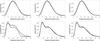Fig. 1 Upper panels: univariate Maxwellian distribution, with parameter σ = 8, is shown with a solid line in all upper panels; black squares connected by dashed lines represent the mean of the nMC = 1000 samples of Tikhonov regularization. Results are for: ns = 30 with σϵ = 0.5 (upper left), ns = 100 with σϵ = 1 (upper center) and ns = 1000 with σϵ = 2 (upper right). Lower panels: bivariate Maxwellian distributions are shown by a solid line in all lower panels, with parameters σ1 = 5 and σ2 = 15 and amplitudes A = 0.7 and B = 0.3. Black squares connected by a dashed line show the estimated PDFs obtained by Tikhonov regularization. Results are for: ns = 30 with σϵ = 0.5 (lower left), ns = 300 with σϵ = 1 (lower center) and ns = 1000 with σϵ = 2 (lower right).

3. Monte Carlo simulation

In this section we present the results of Monte Carlo numerical simulations to assess the performance of the Tikhonov regularization method in deconvolving rotational velocity distribution from the Fredhoml integral. Our Monte Carlo runs consist of n_MC = 1000 independent replications for each chosen scenario, where we considered two specific distributions of rotational velocities. Therefore, we simulate 30 different cases, described as follows:

• a)

  Unimodal distribution: we chose a Maxwellian distribution${\mathit{f}}_{\mathrm{M}}\mathrm{\left(}\mathit{x}\mathrm{\right)}\mathrm{=}\sqrt{\frac{\mathrm{2}}{\mathit{\pi }}}\hspace{0.17em}\frac{\mathrm{1}}{{\mathit{\sigma }}^{\mathrm{3}}}\hspace{0.17em}{\mathit{x}}^{\mathrm{2}}{\mathrm{e}}^{\mathrm{-}\frac{{\mathit{x}}^{\mathrm{2}}}{\mathrm{2}{\mathit{\sigma }}^{\mathrm{2}}}}\mathit{,} \mathit{x}\mathit{>}\mathrm{0}\mathit{,}$(6)with parameter σ = 8, which is the same distribution used in Curé et al. (2014). Furthermore, we considered three different cases, each one including an additive error from a uniform distribution U [−σ_ϵ,σ_ϵ], with PDF given by f_U(x) = 1/(2σ_ϵ) for −σ_ϵ ≤ x ≤ σ_ϵ. The chosen values of σ_ϵ are σ_ϵ = 0.5,1,2 (km s^-1).

• b)

  Bimodal distribution: for a mix of two Maxwellian distributions ${\mathit{f}}_{\mathrm{2}\mathit{M}}\mathrm{\left(}\mathit{x}\mathrm{\right)}\mathrm{=}\sqrt{\frac{\mathrm{2}}{\mathit{\pi }}}\hspace{0.17em}\frac{{\mathit{x}}^{\mathrm{2}}}{\mathit{A}\mathrm{+}\mathit{B}}\left(\frac{\mathit{A}}{{\mathit{\sigma }}_{\mathrm{1}}^{\mathrm{3}}}{\mathrm{e}}^{\mathrm{-}\frac{{\mathit{x}}^{\mathrm{2}}}{\mathrm{2}{\mathit{\sigma }}_{\mathrm{1}}^{\mathrm{2}}}}\mathrm{+}\frac{\mathit{B}}{{\mathit{\sigma }}_{\mathrm{2}}^{\mathrm{3}}}{\mathrm{e}}^{\mathrm{-}\frac{{\mathit{x}}^{\mathrm{2}}}{\mathrm{2}{\mathit{\sigma }}_{\mathrm{2}}^{\mathrm{2}}}}\right)\mathit{,} \mathit{x}\mathit{>}\mathrm{0}\mathit{,}$(7)dispersion parameters are: σ₁ = 5 and σ₂ = 15, and amplitudes: A = 0.3 and B = 0.7. We consider the same additive error cases as for the unimodal distribution.

Furthermore, for both uni- and bimodal cases, we consider five sample lengths n_s: n_s = 30,100,300,1000,10 000.

For each independent Monte Carlo sample two samples needed to be simulated, one from the distribution of the rotational velocities (uni- or bimodal) and another for the kernel, p(y | x), representing the distribution of the inclination angles in the Fredholm integral (Eq. (2)). Then, we multiplied each element of the first sample with the corresponding element of the second sample and added the error term. This gave the final sample of v sin i for each scenario. The following step was to estimate the PDF of the projected rotational velocities with a Kernel Density Estimator (KDE, Silverman 1986). Using a grid of n_g points we discretized the Fredholm integral obtaining the linear system (Eq. (4)). With this data we calculated the Tikhonov factor λ using the procedure described above and obtained the Tikhonov regularization solution, X_λ, which is the estimated PDF of rotational speeds.

Figure 1 upper panels show, using a solid line, the original Maxwellian distribution (Eq. (6)) together with the mean estimated PDF of all Monte Carlo simulations (black squares connected by a dashed line) for different values of σ_ϵ and n_s. It is clearly shown that sample lengths of order n_s ~ 30 give acceptable results when compared with the original sample. For larger sample lengths, n_s ≳ 100, the agreement between the original distribution and the mean of the estimated PDFs is almost exact. Although the mean estimated distribution is slightly shifted to lower velocities. Lower panels of Fig. 1 show the original bimodal mixed Maxwellian distributions (in a solid line) together with the mean estimated PDF (black squares connected by a dashed line). When a sample length is of the order n_s ~ 30, a difference between the estimated PDF and the original PDF is observed. Nevertheless, the Tikhonov regularized solution retrieves the bimodality and delivers ther approximate position of the maximum of both components, but gives a false estimate of the tail of the original distribution.

In the other cases (n_s ≳ 100) the mean of the Tikhonov regularization solutions is very close to the original mixture of Maxwellian distributions, although the estimated value of the amplitudes is slightly lower (first distribution) and slightly higher (second distribution) than the original one.

In order to quantify the error of the estimated PDF, we calculated (following Curé et al. 2014) the mean integrated square error (MISE), that is: $\mathrm{MISE}\mathrm{=}\frac{\mathrm{1}}{{\mathit{n}}_{\mathrm{MC}}}\sum _{\mathit{j}\mathrm{=}\mathrm{1}}^{{\mathit{n}}_{\mathrm{MC}}}\left(\frac{\mathrm{1}}{{\mathit{n}}_{\mathrm{g}}}\sum _{\mathit{i}\mathrm{=}\mathrm{1}}^{{\mathit{n}}_{\mathrm{g}}}\mathrm{\left(}\widehat{{\mathit{f}}_{\mathit{j}}}\mathrm{\right(}{\mathit{x}}_{\mathit{i}}\mathrm{)}\mathrm{-}\mathit{f}\mathrm{(}{\mathit{x}}_{\mathit{i}}\mathrm{)}{\mathrm{)}}^{\mathrm{2}}\right)\mathit{,}$(8)where f(x) represents the original distribution function of rotational speeds and represents the estimated Tikhonov regularization density of the j-run in Monte Carlo simulations.

In the left panel of Fig. 2 we plotted the MISE as a function of sample length for σ_ϵ = 0.5. In the other cases (σ_ϵ = 1, 2) the MISE value is very similar to values MISE ≲ 10^-4. Also it can be seen that as the sample size increases, MISE tends to zero, that is, when n_s → ∞.

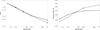Fig. 2 Left panel: value of MISE (black dots) from the estimated PDF for univariate distributions (solid line) and bivariate distributions (dashed line) both using σϵ = 0.5. Right panel: value of Tikhonov factor λ as a function of sample size for the cases where σϵ = 2. See text for details.

The right panel in Fig. 2 shows Tikhonov factor as a function of sample size. These factors are of the same order of magnitude for both types of distribution (uni- and bimodal). Our simulations confirm for all sample lengths and different σ_ϵ values that the Tikhonov factor (λ) is almost independent of the magnitude of the error σ_ϵ. Furthermore, since the Tikhonov parameter changes only slightly as a function of sample size, we can consider the Tikhonov factor as being almost independent of the sample length, n_s.

To confirm this result, we performed MC simulations with a fixed value of λ. The range of λ was from 0.002 to 0.01 with a step of Δ_λ = 0.001. We calculated the MISE from n_MC = 1000 samples, each with a size of n_s = 1000 for each value of λ. For the unimodal Maxwellian distribution the values of the MISE vary, increasing from 7.319 × 10^-5 to 7.320 × 10^-5 for this range of λ, an almost negligible difference. In the case of a bimodal Maxwellian distribution the scenario is very similar. Using the same range of λ, the MISE values vary, increasing from 4.717 × 10^-5 to 4.718 × 10^-5. Similar behaviour is found when n_s = 30,100,300,10 000, supporting our claim that the Tikhonov factor (λ) is almost independent of the sample size.

By means of the average of the estimated PDFs we can estimate the expected value for the Tikhonov regularization solution. In all cases, the mean of the estimated PDFs is very close to the original unimodal or bimodal distributions, and this mean probability density function is closer to the true PDF when increasing the sample size.

This fact shows, empirically, that the studied estimator is asymptotically unbiased. Therefore, since MISE tends to zero when n_s tends to infinity, it is implied that the variance of the Tikhonov regularization estimator tends to zero as well and hence is a consistent estimator.

4. Deconvolving a real sample

In this section, we perform the following steps: (i) apply the Tikhonov regularization method to a sample of measured v sin i data of cluster stars in order to estimate the rotational velocity probability density distribution; and (ii) compare the application of different methods to deconvolve the velocity distribution together with previous non-parametric results from the literature.

4.1. Tarantula sample

We select the Tarantula sample for single O-type stars from the VLT Flames Tarantula Survey, where Ramírez-Agudelo et al. (2013) deconvolved the rotational velocity distribution using the Lucy (1974) method (see also Richardson 1972). This sample contains 216 stars with v sin i data from 40 km s^-1 up to 610 km s^-1. Following Ramírez-Agudelo et al. (2013) for comparison purposes, we also omitted the two largest values (outliers) of the sample. To build the Y vector, we used the KDE method with the following bandwidths (Silverman 1986, pages 45 and 47): $\begin{array}{ccc}{\mathit{h}}_{\mathrm{1}}& \mathrm{=}& \mathrm{0.79}\hspace{0.17em}\mathit{IQR}\hspace{0.17em}{\mathit{n}}_{\mathrm{s}}^{\mathrm{-}\mathrm{1}\mathit{/}\mathrm{5}}\\ {\mathit{h}}_{\mathrm{2}}& \mathrm{=}& \mathrm{0.9}\hspace{0.17em}\begin{array}{c}\min \end{array}\mathrm{\{}\mathrm{\Sigma }\mathit{,IQR}\mathit{/}\mathrm{1.34}\mathrm{\}}\hspace{0.17em}{\mathit{n}}_{\mathrm{s}}^{\mathrm{-}\mathrm{1}\mathit{/}\mathrm{5}}\mathit{,}\end{array}$here, IQR is the interquartile range, Σ is the standard deviation of the sample and n_s is the sample length.

Figure 3 shows, by a solid line, the rotational velocity distribution after Tikhonov regularization. Our procedure for Tikhonov factor determination gives a value of λ = 0.0174 for a step of Δx = 2 km s^-1. Figure 3 also shows the confidence intervals calculated using a bootstrap method (n_BS = 3000, Efron & Tibshirani 1993). The lower is the bandwidth, the wider is the confidence interval. The “bump” around 400 to 450 km s^-1 is wider in our case ranging from 340 km s^-1 to 480 km s^-1. This discrepancy is probably due to the use of the KDE method with a Gaussian kernel in Y.

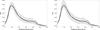Fig. 3 Estimated PDF from the Tarantula sample (solid lines). Both panels with λ = 0.0174 and Δx = 2 km s-1, Left panel with bandwidth h1 = 35.676 and right panel with bandwidth h2 = 30.313. Gray-shaded regions represent the 2.5% (lower) and 97.5% (upper) confidence intervals calculated using a bootstrap method. Dashed lines show the PDF (from Ramírez-Agudelo et al. 2013) obtained using the Lucy (1974) method.

4.2. Comparing results

For the Tarantula sample, we calculate the CDF by direct integration of the PDF obtained via the Tikhonov regularization method and compare this to the CDF calculated using the method described by Curé et al. (2014). Figure 4 shows both CDFs. Their agreement is remarkable. In addition to our results for the PDF, Fig. 3 also shows the PDF (dashed lines) obtained from Ramírez-Agudelo et al. (2013, see their Fig. 17) calculated using the Lucy (1974) method. It can clearly be seen that Lucy-PDF lies inside our confidence interval.

In order to evaluate whether or not both estimated PDFs correspond to the same distribution, we obtained the q–q plot and calculated the respective quantiles. Figure 5 shows the q–q plot of these densities, confirming that both come from the same probability distribution.

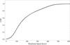Fig. 4 Estimated cumulative rotational velocity distribution function for the Tarantula sample (solid line) obtained using Tikhonov regularization using a spacing of Δx = 2 km s-1 for the velocities. Dots connected by dashed lines show the CDF calculated using the Curé et al. (2014) method with a spacing of Δx = 10 km s-1.

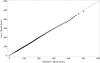Fig. 5 q-q plot from the Tarantula sample, black dots represent the quantiles of each distribution, one calculated using the Tikhonov regularization method and the other calculated using the Lucy method (data from Ramírez-Agudelo et al. 2013).

5. Conclusions

In this work we have obtained the estimated probability distribution function of “true” rotational velocities using the Tikhonov regularization method. Furthermore, this estimated PDF uses a Tikhonov parameter λ obtained by means of an iterative method with a specific stopping criterion in comparison to the widely used iterative method of Lucy (1974).

Through Monte Carlo numerical simulations we assess the proposed method in two cases: when the rotational velocity distribution is described by a Maxwell distribution and for a mixture of two Maxwell distributions. For each situation different scenarios were evaluated obtaining satisfactory results for all of them, except for n_s = 30, when the velocities are described by a mixture of two Maxwellian distributions.

This method retrieves the typical rotational velocity distribution for uni- and bimodal distributions. We showed, empirically, that the studied estimator is asymptotically unbiased and its variance tends to zero. Furthermore, we use the MISE as a measure of goodness of fit of the estimated PDF, which is approximately equal to or less than 10^-4 for all sample sizes and tends to zero when n_s tends to infinity.

We apply this method to a set of observed data from the Tarantula cluster (Ramírez-Agudelo et al. 2013). The estimated PDF from the Tikhonov regularization method agreed very well with the PDF obtained using the Lucy method, as shown by the q-q plot, demonstrating the method’s ability to deconvolve rotational velocities distribution.

In comparison with the method that delivers the CDF described by Cure et al. (2014), Tikhonov regularization solution gives, by direct integration of the PDF, almost the same non–parametric estimation of the true underlying cumulative distribution function of rotational velocities.

To summarize, we previously developed a method to obtain the CDF of “true” rotational velocities (Curé et al. 2014). This current publication presents the Tikhonov regularization method for obtaining the corresponding PDF directly from the Fredhoml integral. Both methods calculate in a simple and straightforward way (PDF, CDF), without any assumptions of the underlying distribution.

Future work: we would like to develop a general function of the kernel of the Fredholm integral, p(y | x), in order to describe an arbitrary orientation of rotational axes. Thus, we can study the distribution of rotational speeds relaxing the standard assumption of uniformity of stellar axes.

Acknowledgments

A.C. thanks the support from the Instituto de Estadística, Pontificia Universidad Católica de Valparaíso. P.E. thanks the support from the Advanced Center for Electrical and Electronic Engineering, AC3E, Basal Fund Conicyt FB0008. M.C. thanks the support from the Centro de Astrofísica de Valparaíso and the Centro Interdiciplinario de Estudios Atmosféricos y Astroestadística. J.C. and D.R. thanks project “Métodos de deconvolución aplicados a la astronomía”, Ministerio de Educación – Secretaría de Políticas and Universitarias, the Universidad Nacional de General Sarmiento and the Universidad de Buenos Aires for their financial support. D.R. also acknowledges the support of the project PIP11420090100165, CONICET.

References

Appendix A: The Tikhonov regularization method

In this Appendix we give a brief description of the Tikhonov regularization method closely following Burger (2007) and Eggermont (1993). Suppose that we have a linear system of the form ${A}\hspace{0.17em}{X}\mathrm{=}{Y}\mathit{,}$(A.1)with a matrix A ∈ R^{n × n}, and vectors X,Y ∈ Rⁿ. Suppose additionally that A is a symmetrical, positive definite matrix. In this case, from spectral theory for symmetrical matrices there exist eigenvalues, 0 <μ₁ ≤ ··· ≤ μ_n and corresponding eigenvectors u_i ∈ Rⁿ, with the euclidean norm | | u_i | | = 1, such that ${A}\mathrm{=}\sum _{\mathit{i}\mathrm{=}\mathrm{1}}^{\mathit{n}}{\mathit{\mu }}_{\mathit{i}}{{u}}_{\mathit{i}}{{u}}_{\mathit{i}}^{\mathit{T}}\mathit{,}$(A.2)where we consider u_i ∈ R^{n × 1}. Since the solution of (A.1) is given by: ${X}\mathrm{=}\sum _{\mathit{i}\mathrm{=}\mathrm{1}}^{\mathit{n}}{\mathit{\mu }}_{\mathit{i}}^{-1}{{u}}_{\mathit{i}}{{u}}_{\mathit{i}}^{\mathit{T}}\mathit{,}$(A.3)small eigenvalues of A can cause numerical difficulties when they are arbitrarily close to zero and the problem is ill-posed. The condition number κ: = μ_n/μ₁, is a measure of the stability of the system. For simplicity we shall assume that μ_n = 1 then κ = 1 /μ₁. When we have data with error Y_δ instead of Y, satisfying | | Y_δ−Y | | <δ, we obtain a solution X_δ and the error in the solution is: $\mathrm{\left|}\mathrm{\right|}{{X}}_{\mathit{\delta }}\mathrm{-}{X}\mathrm{|}{\mathrm{|}}^{\mathrm{2}}\mathrm{=}\sum _{\mathit{i}\mathrm{=}\mathrm{1}}^{\mathit{n}}{\mathit{\mu }}_{\mathit{i}}^{-2}\mathrm{|}{{u}}_{\mathit{i}}^{\mathit{T}}\mathrm{(}{{Y}}_{\mathit{\delta }}\mathrm{-}{Y}\mathrm{)}{\mathrm{|}}^{\mathrm{2}}\mathrm{\le }{\mathit{\mu }}_{\mathrm{1}}^{-2}\mathrm{\left|}\mathrm{\right|}{{Y}}_{\mathit{\delta }}\mathrm{-}{Y}\mathrm{|}{\mathrm{|}}^{\mathrm{2}}\mathit{,}$(A.4)then | | X_δ−X | | ² ≤ κδ.

One observes that with increasing condition number the error amplification increases simultaneously. Often the nature of the error is unknown, then it is necessary used a method to solve the linear system that deals with error effects. The regularization methods face this problem efficiently. If matrix A is positive semi-definite, its eigenvalues are non-negative, but it can have a zero eigenvalue. In this case, let μ_m be the smallest positive eigenvalue, then the solution of (A.1) becomes: ${X}\mathrm{=}\sum _{\mathit{i}\mathrm{=}\mathit{m}}^{\mathit{n}}{\mathit{\mu }}_{\mathit{i}}^{-1}{{u}}_{\mathit{i}}{{u}}_{\mathit{i}}^{\mathit{T}}\mathit{,}$(A.5)and the problem is solvable if and only if ${{u}}_{\mathit{i}}^{\mathit{T}}{Y}\mathrm{=}\mathrm{0}$ for i<m.

For data with error, we can use the projection PY_δ onto the range of A. This analysis can be extended to a general matrix A ∈ R^{n × m} by considering the associated system A^T AX = A^T Y, being that the matrix A^T A is always symmetrical, positive and semi-definite.

In order to shift away from zero the smallest eigenvalues of this matrix A^T A, it seems natural to approximate A^T A for a family of matrices A_λ: = A^T A + λI, whose eigenvalues are μ_i + λ, where μ_is are the eigenvalues of A^T A.

We obtain an approximated solution ${{X}}_{\mathit{\lambda }}\mathrm{=}{{A}}_{\mathit{\lambda }}^{-1}\hspace{0.17em}{{A}}^{\mathit{T}}\hspace{0.17em}{Y}$ and for data with error we have ${{X}}_{\mathit{\lambda ,\delta }}\mathrm{=}{{A}}_{\mathit{\lambda }}^{-1}\hspace{0.17em}{{A}}^{\mathit{T}}\hspace{0.17em}{{Y}}_{\mathit{\delta }}$. The error of the estimation is then $\mathrm{\left|}\mathrm{\right|}{X}\mathrm{-}{{X}}_{\mathit{\lambda ,\delta }}\mathrm{|}{\mathrm{|}}^{\mathrm{2}}\mathrm{\le }\mathrm{|}\mathrm{|}{X}\mathrm{-}{{X}}_{\mathit{\lambda }}\mathrm{|}{\mathrm{|}}^{\mathrm{2}}\mathrm{+}\mathrm{\left|}\mathrm{\right|}{{X}}_{\mathit{\lambda }}\mathrm{-}{{X}}_{\mathit{\lambda ,\delta }}\mathrm{|}{\mathrm{|}}^{\mathrm{2}}\mathit{.}$(A.6)The first term on the right side corresponds to the approximation error and the second term corresponds to the error in data. Using spectral theory (Burger 2007), we obtain: $\mathrm{\left|}\mathrm{\right|}{X}\mathrm{-}{{X}}_{\mathit{\lambda ,\delta }}\mathrm{|}{\mathrm{|}}^{\mathrm{2}}\mathrm{\le }\frac{\mathit{\lambda }}{{\mathit{\mu }}_{\mathrm{1}}\mathrm{(}{\mathit{\mu }}_{\mathrm{1}}\mathrm{+}\mathit{\lambda }\mathrm{)}}\mathrm{(}\mathrm{\left|}\mathrm{\right|}{{Y}}_{\mathit{\delta }}\mathrm{\left|}\mathrm{\right|}\mathrm{+}\mathit{\delta }\mathrm{)}\mathrm{+}\frac{\mathit{\delta }}{\mathrm{(}{\mathit{\mu }}_{\mathrm{1}}\mathrm{+}\mathit{\lambda }\mathrm{)}}\mathrm{·}$(A.7)The first term on the right side decreases when λ tends to zero while the second term on the right side increases when λ tends to zero. Thus, we have to find an estimation of λ that is a compromise between the error of the approximation and the error from measurements.

The solution of the Tikhonov regularization can be obtained also from the Singular Value Descomposition (SVD) of matrix A. In this case, we write a general matrix A ∈ R^{m × n} with rank n in the form: ${{A}}^{\mathit{T}}{A}\mathrm{=}\sum _{\mathit{i}\mathrm{=}\mathrm{1}}^{\mathit{n}}{{u}}_{\mathit{i}}{\mathit{\sigma }}_{\mathit{i}}{\mathit{v}}_{\mathit{i}}^{\mathit{T}}\mathit{,}$(A.8)where u_i and v_i are orthonormal vectors of dimensions m and n respectively, and σ_i ≥ 0 are the singular values of A^T A such that σ₁ ≥ σ₂ ≥ ··· ≥ σ_n> 0. Under this decomposition the Tikhonov solution is given by: ${{X}}_{\mathit{\lambda }}\mathrm{=}\sum _{\mathit{i}\mathrm{=}\mathrm{1}}^{\mathit{n}}{\mathit{f}}_{\mathit{i}}\frac{{{u}}_{\mathit{i}}^{\mathit{T}}{Y}}{{\mathit{\sigma }}_{\mathit{i}}}{\mathit{v}}_{\mathit{i}}\mathit{,}$(A.9)where f_i, i = 1,··· ,n are defined by f_i = σ_i/ (σ_i + λ²).

As we mentioned in Sect. 2 there are several methods to estimate λ. The most frequently used are the L-curve Criterion, the Discrepancy Principle and Generalized Cross Validation.

The L-curve is a plot of $\log \mathrm{\left(}\mathrm{\right|}\mathrm{|}{A}\hspace{0.17em}{{X}}_{\mathit{\lambda }}\mathrm{-}{Y}\mathrm{|}{\mathrm{|}}_{\mathrm{2}}^{\mathrm{2}}\mathrm{)}$ versus $\log \mathrm{\left(}\mathrm{\right|}\mathrm{\left|}{{X}}_{\mathit{\lambda }}\mathrm{\right|}{\mathrm{|}}_{\mathrm{2}}^{\mathrm{2}}\mathrm{)}$, the logarithm of two square euclidean norm, for different values of the Tikhonov factor λ. This plot has the characteristic “L” shape (see Fig. B.1). According to Hansen (2010) the Tikhonov solution X_λ can be decomposed as ${{X}}_{\mathit{\lambda }}\mathrm{=}\overline{{X}}{}_{\mathit{\lambda }}\mathrm{+}{{X}}_{\mathit{\lambda ,e}}$, where $\overline{{X}}{}_{\mathit{\lambda }}\mathrm{=}\mathrm{(}{{A}}^{\mathit{T}}\hspace{0.17em}{A}\mathrm{+}{\mathit{\lambda }}^{\mathrm{2}}\mathit{I}{\mathrm{)}}^{-1}\hspace{0.17em}{{A}}^{\mathit{T}}{Y}$ is the regularized version of the exact solution X, and X_λ,e = (A^T A + λ²I)^-1A^T e is the solution obtained by applying Tikhonov regularization to the error component e. For small values of λ, the error dominates the L-curve because the regularized solution X_λ is dominated by X_λ,e and for large values of λ, X_λ is dominated by $\overline{{X}}{}_{\mathit{\lambda }}$, the unperturbed term. The λ chosen achieves a compromise between the two parts, allocated in the corner of the L-curve. The L-curve criterion for choosing the regularization factor is one of the most frequently used methods. The advantages are robustness and ability to manage observations with correlated errors. The limitations of the L-curve are the reconstruction of very smooth, exact solutions and treatment with a large amount of data (Hansen 2010).

Appendix B: Determination of regularization parameters

When we apply the L-curve method to different v sin i samples, the obtained values of the Tikhonov factor (λ) are “large”. The large size of these values is due to the small values of the coefficients in singular value decomposition with almost constant singular values around 1, requiring the addition of too many terms to increase the norm of X (the vertical part of the “L” shape, see Fig. B.1). We suspect that the reason for this is the smoothness of the solution (Hansen 2010). For the Tarantula sample (Sect. 4), the Tikhonov parameter delivered by the L-Curve, and the GCV methods, are the same, λ = 0.2956.

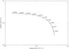Fig. B.1 L-curve plot for the data obtained by the Monte Carlo sample for a unimodal distribution. Horizontal axis shows $\log \mathrm{\left(}\mathrm{\right|}\mathrm{|}{A}\hspace{0.17em}{{X}}_{\mathit{\lambda }}\mathrm{-}{Y}\mathrm{|}{\mathrm{|}}_{\mathrm{2}}^{\mathrm{2}}\mathrm{)}$, i.e., the residuals of the regularization. Vertical axis shows $\log \mathrm{\left(}\mathrm{\right|}\mathrm{\left|}{{X}}_{\mathit{\lambda }}\mathrm{\right|}{\mathrm{|}}_{\mathrm{2}}^{\mathrm{2}}\mathrm{)}$, i.e., the norm of the regularization. Thihkonov parameter values (λ) are overplotted to the corresponding data points. Only the horizontal part of the typical “L” shape is shown. This situation occurs with very smooth exact solutions. See text for details.

Here we show how to determine the value of λ₀ and the choice of factor (f) to select the parameters λ of the Thikhonov method.

As we stated at the end of Sect. 2, we start with an initial value of λ₀ and calculate the Tikonov method to obtain the PDF, (X_λ(1)), then we multiply λ₀ by a factor f and obtain a new value of λ = λ(1) = λ₀ × f, and another PDF (X_λ(2)), after applying Tikhonov method. After “m” iterations we have a set of {λ(1),λ(2),...,λ(m)}.

Defining φ(j) as: 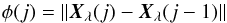$\mathit{\phi }\mathrm{\left(}\mathit{j}\mathrm{\right)}\mathrm{=}\mathrm{\parallel }{{X}}_{\mathit{\lambda }}\mathrm{\left(}\mathit{j}\mathrm{\right)}\mathrm{-}{{X}}_{\mathit{\lambda }}\mathrm{(}\mathit{j}\mathrm{-}\mathrm{1}\mathrm{)}\mathrm{\parallel }$(B.1)where ∥·∥ represents the euclidian norm. After these “m” iterations we also have a set of {φ(2),φ(3),...,φ(m)}. The iteration stops when the value of φ(m) is less than a certain value of ϵ. In our case we chose ϵ = 10^-7.

Figure B.2 shows, log (λ) versus log (φ) for different values of λ₀ and f, for the Tarantula sample. The initial values of λ₀ are: λ₀ = 10, shown as a dotted line in all three curves; λ₀ = 1, shown as dashed lines and λ₀ = 0.1, as solid lines.

For a given value of f, all three curves are superimposed, showing that the final value of λ is independent of the starting value λ₀. Therefore we chose to start our calculations with λ₀ = 0.1. On the other hand, the critical parameter here is f; the lower this value, the lower the final value of λ, when φ(m) ≤ ϵ. Considering that λ is of the order λ² in Eq. (5), a very small parameter λ should be avoided in order to have a non-zero regularization term. Thus we select f = 0.99 as our default value to obtain the Tikhonov parameter λ.

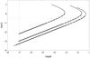Fig. B.2 log (λ) versus log (φ). Factor f varies from f = 0.99 (left), f = 0.75 (center) to f = 0.5 (right). Each of these curves starts with three initial values of λ0, dotted line (λ0 = 10), dashed line (λ0 = 1) and solid line (λ0 = 0.1). See text for details. The vertical gray solid line shows the selected value of ϵ = 10-7 as a criterion to finish the iteration process. The horizontal gray solid line shows the value of λ = 0.2956 (log (λ) = −0.53) obtained using the L–Curve or GCV methods.

It is clearly seen in Fig. B.2, that for log (λ) = −0.53, that is, the value obtained by the L–Curve or GCV method (horizontal gray line) corresponds to a very “high” value of ϵ. If f = 0.99 then ϵ = 1.8 × 10^-4, value much larger than ϵ = 10^-7, which is our criterion to stop this iteration process.

All Figures

Fig. 1 Upper panels: univariate Maxwellian distribution, with parameter σ = 8, is shown with a solid line in all upper panels; black squares connected by dashed lines represent the mean of the nMC = 1000 samples of Tikhonov regularization. Results are for: ns = 30 with σϵ = 0.5 (upper left), ns = 100 with σϵ = 1 (upper center) and ns = 1000 with σϵ = 2 (upper right). Lower panels: bivariate Maxwellian distributions are shown by a solid line in all lower panels, with parameters σ1 = 5 and σ2 = 15 and amplitudes A = 0.7 and B = 0.3. Black squares connected by a dashed line show the estimated PDFs obtained by Tikhonov regularization. Results are for: ns = 30 with σϵ = 0.5 (lower left), ns = 300 with σϵ = 1 (lower center) and ns = 1000 with σϵ = 2 (lower right).

In the text

	Fig. 2 Left panel: value of MISE (black dots) from the estimated PDF for univariate distributions (solid line) and bivariate distributions (dashed line) both using σϵ = 0.5. Right panel: value of Tikhonov factor λ as a function of sample size for the cases where σϵ = 2. See text for details.
In the text

Fig. 3 Estimated PDF from the Tarantula sample (solid lines). Both panels with λ = 0.0174 and Δx = 2 km s-1, Left panel with bandwidth h1 = 35.676 and right panel with bandwidth h2 = 30.313. Gray-shaded regions represent the 2.5% (lower) and 97.5% (upper) confidence intervals calculated using a bootstrap method. Dashed lines show the PDF (from Ramírez-Agudelo et al. 2013) obtained using the Lucy (1974) method.

In the text

	Fig. 4 Estimated cumulative rotational velocity distribution function for the Tarantula sample (solid line) obtained using Tikhonov regularization using a spacing of Δx = 2 km s-1 for the velocities. Dots connected by dashed lines show the CDF calculated using the Curé et al. (2014) method with a spacing of Δx = 10 km s-1.
In the text

	Fig. 5 q-q plot from the Tarantula sample, black dots represent the quantiles of each distribution, one calculated using the Tikhonov regularization method and the other calculated using the Lucy method (data from Ramírez-Agudelo et al. 2013).
In the text

Fig. B.1 L-curve plot for the data obtained by the Monte Carlo sample for a unimodal distribution. Horizontal axis shows $\log \mathrm{\left(}\mathrm{\right|}\mathrm{|}{A}\hspace{0.17em}{{X}}_{\mathit{\lambda }}\mathrm{-}{Y}\mathrm{|}{\mathrm{|}}_{\mathrm{2}}^{\mathrm{2}}\mathrm{)}$, i.e., the residuals of the regularization. Vertical axis shows $\log \mathrm{\left(}\mathrm{\right|}\mathrm{\left|}{{X}}_{\mathit{\lambda }}\mathrm{\right|}{\mathrm{|}}_{\mathrm{2}}^{\mathrm{2}}\mathrm{)}$, i.e., the norm of the regularization. Thihkonov parameter values (λ) are overplotted to the corresponding data points. Only the horizontal part of the typical “L” shape is shown. This situation occurs with very smooth exact solutions. See text for details.

In the text

Fig. B.2 log (λ) versus log (φ). Factor f varies from f = 0.99 (left), f = 0.75 (center) to f = 0.5 (right). Each of these curves starts with three initial values of λ0, dotted line (λ0 = 10), dashed line (λ0 = 1) and solid line (λ0 = 0.1). See text for details. The vertical gray solid line shows the selected value of ϵ = 10-7 as a criterion to finish the iteration process. The horizontal gray solid line shows the value of λ = 0.2956 (log (λ) = −0.53) obtained using the L–Curve or GCV methods.

In the text

References

- Bouhamidi, A., & Jbilou, K. 2007, J. Comput. Appl. Math., 206, 86 [NASA ADS] [CrossRef] [Google Scholar]
- Burger, M. 2007, Inverse Problems, Lecture Notes, Winter 2007/08 (University Muenster) [Google Scholar]
- Chandrasekhar, S., & Münch, G. 1950, ApJ, 111, 142 [NASA ADS] [CrossRef] [MathSciNet] [Google Scholar]
- Curé, M., Rial, D. F., Christen, A., & Cassetti, J. 2014, A&A, 565, A85 [NASA ADS] [CrossRef] [EDP Sciences] [Google Scholar]
- Deng, L.-J., Huang, T.-Z., Zhao, L., & Wang, S. 2013, J. Opt. Soc. Am. A, 30, 5 [Google Scholar]
- Efron, B., & Tibshirani, R. J. 1993, An Introduction to the Bootstrap (Chapman & Hall CRC) [Google Scholar]
- Eggermont, P. P. B. 1993, SIAM J. Math. Anal., 24, 6 [CrossRef] [Google Scholar]
- Fomel, S. 2007, Geophysics, 72, 29 [NASA ADS] [Google Scholar]
- Hansen, P. C. 2010, Discrete Inverse Problems: Insight and Algorithms (SIAM) [Google Scholar]
- Ivanov, V., Vasin, V., & Tanana, V. 2002, Theory of linear ill-posed problems and its applications (Utrecht, Boston: VSP) [Google Scholar]
- Lucy, L. B. 1974, AJ, 79, 745 [NASA ADS] [CrossRef] [Google Scholar]
- Lucy, L. B. 1994, Rev. Mod. Astron., 7, 31 [NASA ADS] [Google Scholar]
- Press, W. H., Teukolsky, S. A., Vetterling, W. T., & Flannery, B. P. 2007, Numerical recipes (Cambridge University Press) [Google Scholar]
- Ramírez-Agudelo, O. H., Simón-Díaz, S., Sana, H., et al. 2013, A&A, 560, A29 [NASA ADS] [CrossRef] [EDP Sciences] [Google Scholar]
- Richardson, W. H. 1972, J. Opt. Soc. America, 62, 55 [Google Scholar]
- Silverman, B. W. 1986, Density estimation for statistics and data analysis. Monographs on Statistics and Applied Probability No. 26 (London: Chapman and Hall) [Google Scholar]
- Tikhonov, A. N. 1943, C. R. (Doklady) Acad. Sci. URSS (N. S.), 39, 176 [Google Scholar]
- Tikhonov, A. N. 1963, Soviet Math Dokl 4, 1035, English translation of Dokl Akad Nauk SSSR, 151, 501 [Google Scholar]
- Tikhonov, A. N., & Arsenin, V. Y. 1977, Solution of Ill-posed Problems (Washington: Winston & Sons) [Google Scholar]
- Tikhonov, A. N., Goncharsky, A. V., Stepanov, V. V., & Yagola, A. G. 1995, Numerical Methods for the Solution of Ill-Posed Problems (Kluwer Academic Publishers) [Google Scholar]