| Issue |
A&A
Volume 595, November 2016
|
|
|---|---|---|
| Article Number | A65 | |
| Number of page(s) | 14 | |
| Section | Extragalactic astronomy | |
| DOI | https://doi.org/10.1051/0004-6361/201628970 | |
| Published online | 31 October 2016 | |
Atomic-to-molecular gas phase transition triggered by the radio jet in Centaurus A⋆,⋆⋆
1 LERMA, Observatoire de Paris, CNRS, UPMC, PSL Univ., 61 avenue de l’Observatoire, 75014 Paris, France
e-mail: This email address is being protected from spambots. You need JavaScript enabled to view it.
2 Collège de France, 11 place Marcelin Berthelot, 75005 Paris, France
3 CRAL, Observatoire de Lyon, CNRS, Université Lyon 1, 9 Avenue Ch. André, 69561 Saint-Genis-Laval Cedex, France
Received: 19 May 2016
Accepted: 29 July 2016
Abstract
NGC 5128 (Centaurus A) is one of the best example to study AGN-feedback in the local Universe. At 13.5 kpc from the galaxy, optical filaments with recent star formation are lying along the radio-jet direction. We used the Atacama Pathfinder EXperiment (APEX) to map the CO(2−1) emission all along the filaments structure. Molecular gas mass of (8.2 ± 0.5) × 107 M⊙ was found over the 4.2 kpc-structure which represents about 3% of the total gas mass of the NGC 5128 cold gas content. Two dusty mostly molecular structures are identified, following the optical filaments. The region corresponds to the crossing of the radio jet with the northern H i shell, coming from a past galaxy merger. One filament is located at the border of the H i shell, while the other is entirely molecular, and devoid of H i gas. The molecular mass is comparable to the H i mass in the shell, suggesting a scenario where the atomic gas was shocked and transformed in molecular clouds by the radio jet. Comparison with combined far-IR Herschel and UV GALEX estimation of star formation rates in the same regions leads to depletion times of more than 10 Gyr. The filaments are thus less efficient than discs in converting molecular gas into stars. Kinetic energy injection triggered by shocks all along the jet and gas interface is a possible process that appears to be consistent with MUSE line ratio diagnostics derived in a smaller region of the northern filaments. Whether the AGN is the sole origin of this energy input and what is the dominant (mechanical vs. radiative) mode for this process is however still to be investigated.
Key words: methods: data analysis / galaxies: individual: Centaurus A / galaxies: evolution / galaxies: star formation / galaxies: interactions / radio lines: galaxies
This publication is based on data acquired with the Atacama Pathfinder Experiment (APEX) under programme ID 096.B-0892.
The reduced APEX spectra (FITS files) are only available at the CDS via anonymous ftp to cdsarc.u-strasbg.fr (130.79.128.5) or via http://cdsarc.u-strasbg.fr/viz-bin/qcat?J/A+A/595/A65
© ESO, 2016
1. Introduction
Understanding the detailed processes involved in the interaction between the interstellar medium (ISM) and intra-cluster medium (ICM) of the radio jets is a key missing piece in the scenario of AGN-regulated galaxy growth. In radio galaxies, interaction between radio jets and the surrounding ISM is suspected to regulate star formation (“negative” feedback; Bower et al. 2006; Croton et al. 2006). But it has also sometimes been claimed to locally enhance the star formation (“positive” feedback; Croft et al. 2006; Bogdán et al. 2011).
Interaction of a jet with molecular gas is very likely to be present along filaments surrounding NGC 5128 (also known as Centaurus A). This giant nearby early-type galaxy lies at the heart of a moderately rich group of galaxies. It hosts a massive disc of dust, gas and young stars in its central regions (Israel 1998). This disc of gas presents a misalignment in CO (Espada et al. 2009), likely due to a recent merger event. The galaxy NGC 5128 is surrounded by faint arc-like stellar shells (at a radius of several kpc around the galaxy) where H i gas has been detected (Schiminovich et al. 1994) and CO emission has been observed at the intersection with the radio jet (Charmandaris et al. 2000). In addition, Auld et al. (2012) detected large amount of dust (~ 105 M⊙) around the northern shell region.
Optically bright filaments are observed in the direction of the radio jet (Blanco et al. 1975; Graham & Price 1981; Morganti et al. 1991). These filaments are thought to be the place of star formation as confirmed by GALEX data (Auld et al. 2012) and young stars (Rejkuba et al. 2001). These so-called inner and outer filaments are located at a distance of ~ 7.7 kpc and ~ 13.5 kpc, respectively. The inner filament lies at the top of the inner radio lobe and could be the result of a weak cocoon-driven bow shock that propagates through the diffuse interstellar medium, triggering star formation (Crockett et al. 2012). Huge X-ray filaments are present in the northern middle radio lobe (Kraft et al. 2009), at the north of the outer filaments, and could result from a jet-cloud interaction where cold, dense clouds have been shock heated to X-ray temperatures. Finally, the inner and outer filaments show distinct kinematical components, a well-defined knotty filament and a more diffuse structure, as highlighted by optical excitation lines (VIMOS and MUSE; Santoro et al. 2015a,b; Hamer et al. 2015). Recently Santoro et al. (2016) identified a star-forming cloud in the MUSE data that contains several H ii regions. Some of these regions are currently forming stars whereas star formation seems to have recently stopped in the others.
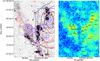 |
Fig. 1 Left: far-UV image of the outer filaments from GALEX (Neff et al. 2015). The black and red contours correspond to the H i and the Herschel-SPIRE 250μm emission (Schiminovich et al. 1994; Auld et al. 2012), respectively. The blue box corresponds the region observed by Charmandaris et al. (2000) with SEST, and the dashed boxes show the field of view of MUSE observations (Santoro et al. 2015b). The circles show the position observed with APEX (CO(2−1) beam). The magenta circles show the non-detections. The regions of Table A.2 are labelled with their number. Right: map of the Herschel-SPIRE 250μm emission. The APEX spectra are overlaid in black. |
In Salomé et al. (2016), we conducted a study of the outer filaments based on archival data. We compared the molecular gas reservoir (via CO with SEST and ALMA archival data) to star-formation tracers far-UV (FUV) with GALEX, far-IR with Herschel. We concentrated on a small region of 130′′ ~ 2 kpc and found that star formation seems to be very inefficient, with large depletion times. In addition, ALMA data revealed the presence of three distinct unresolved and dynamically separated clumps. The virial parameter  (Bertoldi & McKee 1992) of the ALMA clumps (~ 10 − 16) indicates that an input of kinetic energy may have occurred and could explain why these clouds appear inefficient in forming stars despite their surface density NH2 ≥ 1020cm-2. Here we extend this study to larger scales (~ 255′′ ~ 4.2 kpc), based on new CO(2−1) observations with APEX.
For consistency with our previous paper on Centaurus A (Salomé et al. 2016), we used the distance of 3.42 Mpc derived by Ferrarese et al. (2007), leading to a scaling conversion of 16.5pc/′′. However, a recent review of measurements by Harris et al. (2010) has led to a more precise value of 3.8 Mpc. This difference translates into a 10% difference in the spatial scale, and an underestimate of about 20% of the masses and star-formation rates. Nevertheless it does not change the star-formation efficiency (SFE).
2. Observations
Millimetre observations of the CO(2−1) emission were made with the APEX telescope in September 2015 (20 positions) and December 2015 (11 positions). At redshift z = 0.001826, this line is observable at a frequency of 230.118 GHz, which leads to a primary beam of 27.4′′ ~ 450pc. We mapped the whole filaments with 31 pointings. The observations were made with the SHeFI/APEX-1 receiver1 and backends XFFTS (bandwidths of 2.5 GHz; resolution of 88.5 kHz). The typical system temperature was 145 − 180K.
The data were reduced using the IRAM package CLASS. After rejecting bad spectra, a linear baseline was subtracted from the average spectrum; for detections, the baseline was subtracted at velocities outside the range of the emission line. Then, each spectrum was smoothed to a spectral resolution of ~ 12.5 km s-1. During a first run (September), 20 positions were observed with a homogeneous rms of ~ 3mK. Some of the positions were then re-observed (second run) to improve the sensitivity to a rms of ~ 2mK. Finally, 11 new positions were observed during the second run with a rms of ~ 2 − 3mK except if the signal was strong enough (positions 23 and 24). The observations are summarised in Table A.1 and the resulting spectra are plotted in Fig. B.1.
3. Results
3.1. CO emission
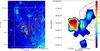 |
Fig. 2 Left: Hα emission of the northern region of Centaurus A with CTIO. The H i emission (VLA; white contours), the CO(2−1) emission (APEX; red contours) and the FUV emission (GALEX; black contours) are overlaid. Right: intensity map of the CO(2−1) emission from APEX in K km s-1, with the H i emission overlaid in black contours. The white box on the left shows the region of the right panel. |
3.1.1. CO detection and star formation
CO emission was detected for 26 of the 31 positions. The CO detections follow the dust emission and are distributed along the UV filaments. The undetected positions are regions 1, 21, 28, 29, and 31 (see Fig. 1 and Table A.2), all of which lie outside the dusty area revealed by Herschel. Region 1 is at the top-north, close to the ALMA detected clumps, in a region where the CO emission is fading, at the edge of the dusty area. Region 21 is between two main east vs. west CO-bright regions. This suggests that those two main regions are clearly separated. However the nearby region 22 is well-detected in CO. The two branches of the northern filaments seen in the optical may thus hide an underlying continuous molecular reservoir. More sensitive observations will confirm this possibility. Regions 28, 29, 31 constitute a continuous north-south region at the very bottom tip of the filaments. The southern part of the filaments seems to be CO free or at least CO poor. One region (30) is however detected in this structure. It corresponds to the position of the only bright star-forming UV-clump of the southern structure.
Some positions detected in CO do not show UV emission, probably due to dust extinction. In addition, positions 16−20 and 23−25 also present Hα emission (CTIO; see Fig. 2). But the lack of Hα emission in the rest of the filaments can be explained by the narrow-band filter of CTIO, the emission being outside the observing band. CO emission is stronger in the eastern part of the filaments (right panel of Fig. 1). The larger molecular mass (9 − 12 × 106 M⊙) that we derived in this eastern region indicates that several giant molecular clouds (GMC) associations are located there.
Estimating the  with the formula from Solomon et al. (1997) and the CO(2−1)/CO(1−0) ratio of 0.55 from Charmandaris et al. (2000), and applying a standard Milky Way αCO = 4.6M⊙ (K km s-1pc2)-1 (Solomon et al. 1997), we derived molecular gas masses of a few 105 − 107 M⊙. For non-detections, we calculated an upper limit at 3σ with a line width of 30 km s-1, similar to the neighbours’ positions.
The star-formation rate (SFR) has been derived from the FUV (GALEX) and IR (Herschel) emission in regions of 27.4′′ too (see Salomé et al. (2016) for the details). We also derived the molecular depletion times,  , of all the APEX positions. Detailed results for each position are summarised in Tables A.2 and A.3. In the whole region that has been observed with APEX, we found a total molecular gas mass MH2 = (8.2 ± 0.5) × 107 M⊙, about five times higher that the mass found by Charmandaris et al. (2000). Although the region presented here is larger than that of Charmandaris et al. (2000), we did not expect such a difference in mass as they observed the peak of H i emission. The difference comes from the large amount of gas found outside the H i cloud. A combination of the IR and FUV emission gives a star-formation rate SFR = (1.08 ± 0.12) × 10-3 M⊙yr-1. This gives a molecular depletion time in the filaments tdep = 75.5 ± 13.0Gyr, indicating that the star formation is very inefficient in the filaments.
3.1.2. Comparison between ALMA and APEX data
Position 1 has the same coordinates as the ALMA data published by Salomé et al. (2016). However, the three detected clumps lie outside the primary beam of ALMA. They are therefore contained in position 2. The ALMA emission was claimed to be SCOΔv ~ 3.0 Jy km s-1 and the position 2 with APEX has an intensity ICO ~ 0.636K km s-1. The APEX Jy/K conversion factor of 32.5 gives a CO flux SCOΔv ~ 20.7 Jy km s-1 thus the ratio of the APEX and ALMA fluxes is approximately seven. If we assume that the CO emission only consists of clumps then there could be approximately seven times more clumps in the APEX beam. Therefore position 2 would contain approximately 21 clumps of mass ~ 5 × 10⁴ M⊙2. The ALMA data can resolve spatial scales up to ~ 18′′ (baselines of 18.4 − 250.8m) therefore the signal is unlikely filtered by the small baseline coverage.
3.1.3. Molecular-to-atomic mass ratio
The outer filaments lie in projection at the interface between the radio jet of Centaurus A and the H i shell. Using the VLA data from Schiminovich et al. (1994), we could derive H2/H i mass ratios at different positions in the filaments. As the resolution of the VLA data (40′′ × 78′′) is lower than the APEX data, we combined several pointings from APEX that are contained in a single VLA beam. The eastern part of the filaments was not detected in H i therefore we used the rms of 2 mJy and a line width of 80 km s-1 (Schiminovich et al. 1994) to derive upper limits at 3σ. We conclude that the filaments are mostly molecular (see Table 1), except for positions 12−14 and 26−27 which lie outside the UV emitting region.
H i and H2 masses in combinations of APEX pointings.
3.1.4. Probability distribution function
We derived the probability distribution function (PDF) of the H2 column density of the APEX pointings (Fig. 3), following Druard et al. (2014). For the 31 APEX pointings, we derived the column density by assuming an homogeneous emission over 450 × 450pc2. Even if there is very few statistics and a lack of resolution, the PDF starts to follow a log-normal distribution: 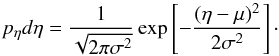 (1)The best fitting result characterises the log-normal by the mean μ = − 0.80 and standard deviation σ = 0.96. The log-normal shape of the PDF indicates that the structure of the molecular gas is dominated by turbulence. However, we do not have a enough statistical sample at small scales to determine the contribution of gravitation (power-law). This will be possible by resolving the GMC at high resolution with forthcoming ALMA observations.
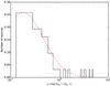 |
Fig. 3 Probability distribution function of the H2 column density of the APEX pointings. The x-axis shows the normalised column density. The red dashed line shows the best fitting log-normal function (Eq. (1)) with σ = 0.96 and μ = − 0.80. |
3.2. An inefficient star formation
We calculated molecular gas and SFR surface densities (ΣH2, ΣSFR) for all the positions (see Table A.3). Both quantities were smoothed over the APEX 27.4′′ beam. We then plotted the ΣSFR vs. ΣH2 diagram (Fig. 4). As mentioned before, the star formation seems very inefficient, with depletion times of the order of tens of Gyr. Nevertheless, the positions seem to follow a Schmidt-Kennicutt law  (Kennicutt 1998), lying lower than star-forming spiral galaxies.
The outer filaments of Centaurus A contain large amounts of molecular gas with a small SFE. Thus star formation is rather inefficient in the filaments. However, star-formation tracers like dust and UV emission are definitely detected, and only detected in the filaments. The presence of young stars (Rejkuba et al. 2001) also indicates that these regions are the place of recent star formation, triggered in a fairly large molecular gas reservoir.
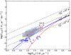 |
Fig. 4 ΣSFR vs. ΣH2 for the different regions of CO emission observed with APEX (blue). The black crosses correspond to the central galaxy and the entire filaments (ΣH2 ~ 16.4M⊙pc-2; ΣSFR ~ 2.17 × 10⁻⁴ M⊙yr-1kpc-2). The diagonal dashed lines show lines of constant molecular gas depletion times of, from top to bottom, 108, 109, and 1010yr. We overlay the contours of Leroy et al. (2013) for nearby spiral galaxies. The red and blue lines represent Eq. (2) for the different set of parameters presented below. |
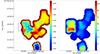 |
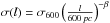
Fig. 5 Peak velocity (left) and velocity dispersion (right) map of the CO(2−1) emission from APEX. The velocities are relative to the systemic 547 km s-1 value. In the left panel, the boxes represent the fields of view observed with VIMOS (small; Santoro et al. 2015a) and MUSE (large; Santoro et al. 2015b). |
Renaud et al. (2012) developed a model to study the effect of turbulence on the SFE. We adapted their model by hypothesising that the SFR volume density ρSFR is simply proportional to the molecular gas volume density: ρSFR = ϵSFEρH2 above a threshold gas density ρ0. Without stellar feedback, the theoretical law between ΣSFR and ΣH2 for a gas distribution given by Eq. (1) is: 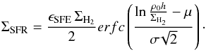 (2)We fixed ϵSFE = 1/2 × 109yr-1 and h = 450pc (the size of the APEX beam), and explore different set of parameters (σ, μ, ρ0). We found that the region with the larger depletion times (the massive regions in the east) are best fitted by σ = 1.5, μ = 0.58, ρ0 = 100cm-3, whereas the region in the west may be fitted by σ = 2.5, μ = 4.58, ρ0 = 103cm-3. However the fits are highly degenerate and different sets of parameters may fit the same regions (e.g. the blue dashed line in Fig. 4). This analysis needs better constraints on the PDF that will then constrain the parameters of Eq. (2).
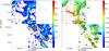 |
Fig. 6 Left: Hα-[N ii] flux map, with the GALEX FUV emission overlaid in black contours. Right: peak velocity map of the Hα-[N ii] emission from MUSE, relative to Centaurus A. The contours shows the Hα-[N ii] flux. The field of view of the MUSE data corresponds to the larger blue boxes in Fig. 5. The APEX 27.4′′ beams are represented by the circles. |
3.3. Dynamics and morphology of the filaments
The overall CO(2−1) emission of the filaments is blueshifted compared to the central galaxy with peak velocities between − 200 and − 300 km s-1 in Centaurus A rest frame (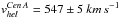 ; Graham 1978). The filaments show velocity gradients (Fig. 5), where the northern part of the filaments has the highest blueshifted velocities with respect to the systemic velocity. The eastern part presents higher velocities (v = − 244.8 km s-1) than the western region (v = − 205.7 km s-1). The CO(2−1) emission is also broader in the east with ⟨Δv⟩ = 69.7 km s-1, whereas the average velocity dispersion in the west is Δv = 42.5 km s-1. It is difficult to distinguish whether the velocity dispersion is produced by turbulence or by the proper motion of several clouds along the line of sight. The larger molecular mass (a few 106 M⊙) combined with the broad emission lines in the east of the filaments indicates that the second solution is more probable. Incoming ALMA data will provide a clear view of the clump distribution.
The APEX pointings do not accurately cover the MUSE observations. Nevertheless we observed part of the Hα emission (Fig. 6). The right panel of Fig. 6 shows the velocity of the Hα-[N ii] emission, relative to Centaurus A. At the location of the CO emission, part of the Hα emission presents velocities of the order of the CO emission ones. The molecular and ionised components may thus be spatially and dynamically associated. A more accurate correlation requires a more homogeneous coverage of the CO emission at similar spatial resolution to that of the MUSE data.
Oosterloo & Morganti (2005) computed a position-velocity (PV) diagram of the H i gas along a slit oriented perpendicularly to the jet. The H i cloud shows a velocity gradient all along its extension. At a distance of 30′′ − 60′′ from the centre of the slit, the authors found a change in the slope of the velocity gradient that they interpreted as a direct effect of the jet interaction with the H i. The CO data along the same slit (Fig. 7) show that (1) the large scale H i velocity gradient is also seen in CO and that it seems to extend further out to the east side as shown by the bright CO spot at ~ 120′′ (following the dashed line); (2) the break in the slope of the H i velocity gradient is also seen in CO. Molecular and atomic gas thus seems to be dynamically associated.
If, as claimed by Oosterloo & Morganti (2005) and Santoro et al. (2015a), the change in velocity is due to the interaction of the radio-jet with the gas, then the gas projected velocity deceleration also affects the molecular components. The jet is expected to accelerate the gas but, a simple change in the orientation of the gas velocity vector induced by the jet can explain this behaviour, the higher velocity having a smaller projection along the line of sight.
3.4. Excitation of the filaments
The optically bright part of the outer filaments was observed with the Multi Unit Spectroscopic Explorer (MUSE) on the VLT (Henault et al. 2003) during the Science Verification period (Program 60.A-9341(A) on 25 June 2014, Santoro et al. 2015b). The observations consisted of two fields, each consisting of three pointings (6 pointings in total) of 1000s each, with a 90°rotation between each. We took the data from the archive and reduced them with version 0.18.1 of the MUSE data reduction pipeline and the European Southern Observatory Recipe Execution Tool (ESOREX v. 3.10.2) command-line interface. The final data cube was then sky subtracted using a 20′′ × 20′′ region of the FOV free from line emission and stars to produce the sky model. We extracted a cube that covers a velocity range of 120 000 km s-1. This cube covers all of the principal line complexes with a constant spectral sampling of 0.6Å (~ 30 km s-1 at the wavelength of Hα). We also extracted an individual cube that covers the Hα-[N ii] lines in the velocity range − 700 to 250 km s-1, relative to the systemic 547 km s-1 value. This velocity range covers the three components identified by Santoro et al. (2015b), here in Fig. 6. We corrected for pointing offsets after the rotation by matching the positions of bright stars within the field of view before combining the pointings from each field. The two fields were then combined to produce a single data cube.
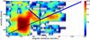 |
Fig. 7 PV diagram of the CO emission (in mK) centred in α = 13h26m15s, δ = −42:49:00 over the same slit orientation as Oosterloo & Morganti (2005) with a width of 4.2′ (taking all the CO emission). The blue lines represent the H i cloud velocity gradient. The dashed line represents the continuity of this velocity gradient over the CO emission. The position of the radio jet is shown by the vertical black line. |
We computed pixel-by-pixel BPT diagrams based on the Hα, [N ii], Hβ, [O iii], [O i] and [S ii] lines (Fig. 8; Baldwin et al. 1981; Kewley et al. 2006). We aimed to look at the distribution of the excitation processes. Each line was fitted by a Gaussian at each spatial resolution element (see Hamer et al. 2014, for the details) in order to measure the flux. Figure 10 shows maps of the different regions regarding the excitation process. Most of the filaments seem to be excited by energy injection from the radio jet or shocks. Those large regions contains smaller inclusions that are excited by star formation, similar to that has been claimed by Santoro et al. (2016). The star-forming regions spatially coincide with the filaments seen in FUV with GALEX. Conversely, the regions excited by the radio jet or shocks are brighter in Hα. Optical line ratios were then extracted only in the velocity range corresponding to the CO velocities. Those optical diagnostics show that the gas is excited by AGN/shocks in some APEX pointings, and excited by star formation in others. Both processes are at play in position 25. The star-forming region of Santoro et al. (2016) is spatially and dynamically coincident with molecular gas in position 20.
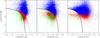 |
Fig. 8 Pixel-by-pixel BPT diagrams of the filaments with MUSE. The black line in the left panel represents the empirical separation of star formation (green) and AGN/shock-ionised regions (blue). The dotted line on the left and the solid lines in the other panels show the extreme upper limit for star formation (Kewley et al. 2006). The red points correspond to the composite regime. |
4. Discussion
The low star formation efficiency – We found in Fig. 4 that the depletion time of the molecular gas in the filaments was longer than the Hubble time. This means a very low efficiency of forming stars with respect to discs. It must be emphasised, however, that the geometry of the filaments is far from disc-like. Molecular gas is clumpy along filaments that are distributed in a larger volume than discs. Therefore the density of filaments is probably small in the northern shell. The average total gas volumic density must be smaller than the typical volume density in galactic disc. The efficiency is also likely to depend on the pressure and the surface density of star (e.g. Blitz & Rosolowsky 2006), which is, on average, low in the filaments. With respect to the H i shell outside the radio jet, the impact of the AGN has been to convert the gas from the H i to H2 phase, and to increase its SFE anyway.
Metallicity effects – The CO/H2 conversion factor is known to be linked to the metallicity. At low metallicity, a standard αCO would underestimate the mass of the molecular gas (Wolfire et al. 2010). In a previous paper (Salomé et al. 2016), we corrected the αCO factor following the method by Leroy et al. (2013), by assuming a constant oxygen abundance within the filaments. However, we show in this paper that the physical conditions of the gas are not uniform in the filaments. Therefore the metallicity may be subject to significant variations, leading to a different αCO along the filaments. Nevertheless, the metallicity ranges deduced from MUSE data are always subsolar (Salomé et al. 2016), so the corresponding αCO should be equal or larger than the standard value we used. The molecular gas masses derived here are thus at worst underestimated leading to even less efficient star formation in the filaments.
Star formation tracers – The star formation rate was estimated by a combination of the IR and FUV emission, the FUV being emitted by massive young OB stars, and the IR being the thermal emission of dust (Kennicutt & Evans 2012, and references therein). However, dust absorbs both the FUV and Hα emission so part of dust heating is likely due to the jet or shock excitation, and not related to star formation. Therefore the star formation rates may be overestimated, leading to the same conclusion as above.
Influence of resolution – Resolution may have effects on the star formation law. Schruba et al. (2010) showed that, at resolution smaller than a few hundreds parsecs, molecular gas and star-formation tracers start to be spatially decorrelated therefore, depending on which regions the aperture is centred (CO emission or star formation tracers), the dependence of ΣSFR on ΣH2 will vary significantly. By combining APEX beams to simulate lower resolutions, we did not find significant change of the depletion time when changing the resolution, contrary to Schruba et al. (2010).
We then explored the evolution of the scatter of log tdep with the resolution. Leroy et al. (2013) derived the relation  where the index β is related to the correlation of star formation with the environment. We calculated the scatter of log tdep in the east and west of the filaments separately, for different combinations of the APEX beams. We found that the APEX pointings in the eastern filament are forming star rather independently (β ~ 0.9) whereas star formation in the west seems to be correlated with the environment (β ~ 0.35) (see Fig. 9 and Leroy et al. 2013, for the details). This tends to indicate that the radio jet could play a more important role in star formation in the western part of the filaments.
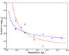 |
Fig. 9 Rms scatter in |

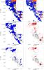 |
Fig. 10 Map of the excitation processes in the field of view of MUSE. Top: RGB map with star formation in green, AGN or shocks in blue, composite in red. The contours show the UV emission from GALEX (black; left) and the Hα-[N ii] emission from MUSE (white; right). Middle: separation of the AGN or shocks excitation (left), and the SF+composite excitation (right). Bottom: separation of the AGN or shocks excitation (left), and the SF+composite excitation (right) for the velocity range of the CO emission (− 256.8 <v< − 194.5 km s-1; relative to Centaurus A). The APEX beams are represented by the circles. |
5. Conclusion
The Atacama Pathfinder EXperiment (APEX) was used to map the full region of Centaurus A’s northern filaments (5′ × 4′). This map follows the optical, UV and dusty elongated structure. At a distance of 13.5 kpc from NGC 5128, the observed region is ~ 4.2 kpc-long. The CO(2−1) emission is detected with a resolution of 450 pc in almost all the 31 targeted positions. The undetected regions are lying at the edges of the filaments and deeper observations will determine the accurate limits of emission where the signal is seen to be fading away. The molecular gas mass is found to lie in two separated prominent structures: the eastern region (the brightest) and the western region. Those two structures follow the optically identified east and west arms of the northern filaments. Emission is however found in between these two filaments (region 22) suggesting a possibly larger underlying cold molecular gas reservoir. The southern tip of the filaments, where a large UV spot lies, is much more CO-poor. This region lies at the edge of the H i shell. The low molecular gas mass may therefore be explained by the gas-poor nature of the region. It might also be explained by a high ionisation of gas, although no clue supports this hypothesis.
Charmandaris et al. (2000) pointed and found CO emission in the H i cloud only (called shell S1 and S2). The CO emission is in fact: (i) much more extended and following the whole optical filaments; (ii) approximately five times more massive with (8.2 ± 0.5) × 107 M⊙ in the whole filaments versus 1.7 × 10⁷ M⊙ in Shell S1 only. The filaments molecular content represents about 3−5% of the total gas mass of the entire galaxy, 1.4 − 2.7 × 10⁹ M⊙ found by Herschel and CO mapping (Parkin et al. 2012); (iii) mostly molecular with a small atomic-to-molecular gas fraction and with the brightest emission being far outside the H i cloud itself. All the CO(2−1)-detected regions are found to be dust-rich.
Archival Herschel far-UV and GALEX UV data were used to determine the star formation rates inside the CO-detected regions. After discussing possible effects of spatial resolution and metallicity, we conclude that the SFE is very low in the northern filaments. Even if traces of recent star formation are claimed in this region (with the presence of young stars), the mass of the molecular gas reservoir available is huge compared to standard SFE. This suggests that some processes may prevent the star formation to proceed in the cold gas. Statistical studies with higher resolution CO data all along the filaments are underway (ALMA cycle 3 project) and will shed light on possibly local effects. Salomé et al. (2016) analyses of very first ALMA archival data already showed that the molecular gas is clumpy and likely not gravitationally bounded. New ALMA data will be used to study whether this tendency extends to the whole filaments or not, as well as the very first trends determined here in the CO mass distribution function. High spatial resolution mapping of the linewidths distribution will also help identifying the star formation quenching mechanism.
A possible process that may prevent the molecular gas to form stars is kinetic energy injection from the larger scale dynamics at play in this system. The CO velocity field found with APEX is consistent with the recent findings (Oosterloo & Morganti 2005; and VIMOS data from Santoro et al. 2015a) of shears in the filaments that may be interpreted as a direct effect of the AGN-jet interaction on the underlying gas distribution. The comparison with MUSE data clearly shows the presence of different excitation mechanisms, AGN and/or shocks being the dominant process in the northern filaments, with localised H ii dominated regions.
The low SFE of the molecular filaments, with respect to discs, might also be interpreted by a volumic effect. Discs are much thinner that the gaseous shell in the halo of Centaurus A, and therefore the molecular gas density lower in average, for the same surface density. Maybe the most interesting impact of the radio jet on the gaseous shell is to compress the gas and trigger the phase transition from atomic to molecular gas. Outside of the radio jet, the fraction of H2 gas was only of the order of 0.2, while the gas had become entirely molecular in the jet. A radio-jet H i ram pressure stripping scenario is unlikely to explain the unbalanced H2/H i ratio in the two filaments. In such a case, the molecular gas content is expected to be the same between the western and eastern filaments. Conversely, we found a much larger amount of molecular gas in the eastern filaments (atomic-free). This is certainly the way the AGN and its jets can have a positive feedback effect on the star formation in NGC 5128.
Note added in proof. After the submission of this paper, we became aware of a similar study by Morganti et al. (2016) with APEX, although with fewer data.
As discussed in a corrigendum, there is a mistake in Salomé et al. (2016). We underestimated the mass of the clumps as we forgot to take into account the CO(2−1)/CO(1−0) ratio.
Acknowledgments
We thank Carlos de Breuck, Katharina Immer and APEX operators for their support for the observations. We also thank the referee for helpful comments.
The Atacama Pathfinder EXperiment (APEX) is a collaboration between the Max-Planck-Institut für Radioastronomie, the European Southern Observatory, and the Onsala Space Observatory.
Based on observations made with ESO Telescopes at the La Silla Paranal Observatory under programme 60.A-9341A.
We acknowledge financial support from “Programme National de Cosmologie and Galaxies” (PNCG) of CNRS/INSU, France.
References
- Auld, R., Smith, M. W. L., Bendo, G., et al. 2012, MNRAS, 420, 1882 [NASA ADS] [CrossRef] [Google Scholar]
- Baldwin, J. A., Phillips, M. M., & Terlevich, R. 1981, PASP, 93, 5 [NASA ADS] [CrossRef] [EDP Sciences] [Google Scholar]
- Bertoldi, F., & McKee, C. F. 1992, ApJ, 395, 140 [NASA ADS] [CrossRef] [Google Scholar]
- Blanco, V. M., Graham, J. A., Lasker, B. M., & Osmer, P. S. 1975, ApJ, 198, L63 [NASA ADS] [CrossRef] [Google Scholar]
- Blitz, L., & Rosolowsky, E. 2006, ApJ, 650, 933 [NASA ADS] [CrossRef] [Google Scholar]
- Bogdán, A., Kraft, R. P., Forman, W. R., et al. 2011, ApJ, 743, 59 [NASA ADS] [CrossRef] [Google Scholar]
- Bower, R. G., Benson, A. J., Malbon, R., et al. 2006, MNRAS, 370, 645 [NASA ADS] [CrossRef] [Google Scholar]
- Charmandaris, V., Combes, F., & van der Hulst, J. M. 2000, A&A, 356, L1 [NASA ADS] [Google Scholar]
- Crockett, R. M., Shabala, S. S., Kaviraj, S., et al. 2012, MNRAS, 421, 1603 [NASA ADS] [CrossRef] [Google Scholar]
- Croft, S., van Breugel, W., de Vries, W., et al. 2006, ApJ, 647, 1040 [NASA ADS] [CrossRef] [Google Scholar]
- Croton, D. J., Springel, V., White, S. D. M., et al. 2006, MNRAS, 365, 11 [NASA ADS] [CrossRef] [Google Scholar]
- Druard, C., Braine, J., Schuster, K. F., et al. 2014, A&A, 567, A118 [NASA ADS] [CrossRef] [EDP Sciences] [Google Scholar]
- Espada, D., Matsushita, S., Peck, A., et al. 2009, ApJ, 695, 116 [NASA ADS] [CrossRef] [Google Scholar]
- Ferrarese, L., Mould, J. R., Stetson, P. B., et al. 2007, ApJ, 654, 186 [NASA ADS] [CrossRef] [Google Scholar]
- Graham, J. A. 1978, PASP, 90, 237 [NASA ADS] [CrossRef] [Google Scholar]
- Graham, J. A., & Price, R. M. 1981, ApJ, 247, 813 [NASA ADS] [CrossRef] [Google Scholar]
- Hamer, S., Salomé, P., Combes, F., & Salomé, Q. 2015, A&A, 575, L3 [NASA ADS] [CrossRef] [EDP Sciences] [Google Scholar]
- Hamer, S. L., Edge, A. C., Swinbank, A. M., et al. 2014, MNRAS, 437, 862 [NASA ADS] [CrossRef] [Google Scholar]
- Harris, G. L. H., Rejkuba, M., & Harris, W. E. 2010, PASA, 27, 457 [NASA ADS] [CrossRef] [Google Scholar]
- Henault, F., Bacon, R., Bonneville, C., et al. 2003, in Instrument Design and Performance for Optical/Infrared Ground-based Telescopes, eds. M. Iye, & A. F. M. Moorwood, 4841, 1096 [Google Scholar]
- Israel, F. 1998, A&ARv, 8, 237 [NASA ADS] [CrossRef] [Google Scholar]
- Kennicutt, Jr., R. C. 1998, ApJ, 498, 541 [NASA ADS] [CrossRef] [Google Scholar]
- Kennicutt, R. C., & Evans, N. J. 2012, ARA&A, 50, 531 [NASA ADS] [CrossRef] [Google Scholar]
- Kewley, L. J., Groves, B., Kauffmann, G., & Heckman, T. 2006, MNRAS, 372, 961 [NASA ADS] [CrossRef] [Google Scholar]
- Kraft, R. P., Forman, W. R., Hardcastle, M. J., et al. 2009, ApJ, 698, 2036 [NASA ADS] [CrossRef] [Google Scholar]
- Leroy, A. K., Walter, F., Sandstrom, K., et al. 2013, AJ, 146, 19 [NASA ADS] [CrossRef] [Google Scholar]
- Morganti, R., Robinson, A., Fosbury, R. A. E., et al. 1991, MNRAS, 249, 91 [NASA ADS] [Google Scholar]
- Morganti, R., Oosterloo, T., Oonk, J. B. R., Santoro, F., & Tadhunter, C. 2016, A&A, 592, L9 [NASA ADS] [CrossRef] [EDP Sciences] [Google Scholar]
- Neff, S. G., Eilek, J. A., & Owen, F. N. 2015, ApJ, 802, 88 [NASA ADS] [CrossRef] [Google Scholar]
- Oosterloo, T. A., & Morganti, R. 2005, A&A, 429, 469 [NASA ADS] [CrossRef] [EDP Sciences] [Google Scholar]
- Parkin, T. J., Wilson, C. D., Foyle, K., et al. 2012, MNRAS, 422, 2291 [NASA ADS] [CrossRef] [Google Scholar]
- Rejkuba, M., Minniti, D., Silva, D. R., & Bedding, T. R. 2001, A&A, 379, 781 [NASA ADS] [CrossRef] [EDP Sciences] [Google Scholar]
- Renaud, F., Kraljic, K., & Bournaud, F. 2012, ApJ, 760, L16 [NASA ADS] [CrossRef] [Google Scholar]
- Salomé, Q., Salomé, P., Combes, F., Hamer, S., & Heywood, I. 2016, A&A, 586, A45; Corrigendum, 593, C5 [NASA ADS] [CrossRef] [EDP Sciences] [Google Scholar]
- Santoro, F., Oonk, J. B. R., Morganti, R., & Oosterloo, T. 2015a, A&A, 574, A89 [NASA ADS] [CrossRef] [EDP Sciences] [Google Scholar]
- Santoro, F., Oonk, J. B. R., Morganti, R., Oosterloo, T. A., & Tremblay, G. 2015b, A&A, 575, L4 [NASA ADS] [CrossRef] [EDP Sciences] [Google Scholar]
- Santoro, F., Oonk, J. B. R., Morganti, R., Oosterloo, T. A., & Tadhunter, C. 2016, A&A, 590, A37 [NASA ADS] [CrossRef] [EDP Sciences] [Google Scholar]
- Schiminovich, D., van Gorkom, J. H., van der Hulst, J. M., & Kasow, S. 1994, ApJ, 423, L101 [NASA ADS] [CrossRef] [Google Scholar]
- Schruba, A., Leroy, A. K., Walter, F., Sandstrom, K., & Rosolowsky, E. 2010, ApJ, 722, 1699 [NASA ADS] [CrossRef] [Google Scholar]
- Solomon, P. M., Downes, D., Radford, S. J. E., & Barrett, J. W. 1997, ApJ, 478, 144 [NASA ADS] [CrossRef] [Google Scholar]
- Wolfire, M. G., Hollenbach, D., & McKee, C. F. 2010, ApJ, 716, 1191 [NASA ADS] [CrossRef] [Google Scholar]
Appendix A: Additional tables
Journal of observations with APEX.
CO luminosities and molecular masses in the regions observed with APEX.
Molecular gas masses, SFR and  in regions of 27′′ around the APEX pointings.
Appendix B: APEX spectra of CO(2−1) emission
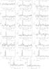 |
Fig. B.1 CO(2−1) spectra of all the positions observed with APEX. The vertical blue and red lines indicate velocities of − 300 and − 200km.s-1. |
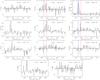 |
Fig. B.1 continued. |
All Tables
All Figures
|
Fig. 1 Left: far-UV image of the outer filaments from GALEX (Neff et al. 2015). The black and red contours correspond to the H i and the Herschel-SPIRE 250μm emission (Schiminovich et al. 1994; Auld et al. 2012), respectively. The blue box corresponds the region observed by Charmandaris et al. (2000) with SEST, and the dashed boxes show the field of view of MUSE observations (Santoro et al. 2015b). The circles show the position observed with APEX (CO(2−1) beam). The magenta circles show the non-detections. The regions of Table A.2 are labelled with their number. Right: map of the Herschel-SPIRE 250μm emission. The APEX spectra are overlaid in black. |
| In the text | |
|
Fig. 2 Left: Hα emission of the northern region of Centaurus A with CTIO. The H i emission (VLA; white contours), the CO(2−1) emission (APEX; red contours) and the FUV emission (GALEX; black contours) are overlaid. Right: intensity map of the CO(2−1) emission from APEX in K km s-1, with the H i emission overlaid in black contours. The white box on the left shows the region of the right panel. |
| In the text | |
|
Fig. 3 Probability distribution function of the H2 column density of the APEX pointings. The x-axis shows the normalised column density. The red dashed line shows the best fitting log-normal function (Eq. (1)) with σ = 0.96 and μ = − 0.80. |
| In the text | |
|
Fig. 4 ΣSFR vs. ΣH2 for the different regions of CO emission observed with APEX (blue). The black crosses correspond to the central galaxy and the entire filaments (ΣH2 ~ 16.4M⊙pc-2; ΣSFR ~ 2.17 × 10⁻⁴ M⊙yr-1kpc-2). The diagonal dashed lines show lines of constant molecular gas depletion times of, from top to bottom, 108, 109, and 1010yr. We overlay the contours of Leroy et al. (2013) for nearby spiral galaxies. The red and blue lines represent Eq. (2) for the different set of parameters presented below. |
| In the text | |
|
Fig. 5 Peak velocity (left) and velocity dispersion (right) map of the CO(2−1) emission from APEX. The velocities are relative to the systemic 547 km s-1 value. In the left panel, the boxes represent the fields of view observed with VIMOS (small; Santoro et al. 2015a) and MUSE (large; Santoro et al. 2015b). |
| In the text | |
|
Fig. 6 Left: Hα-[N ii] flux map, with the GALEX FUV emission overlaid in black contours. Right: peak velocity map of the Hα-[N ii] emission from MUSE, relative to Centaurus A. The contours shows the Hα-[N ii] flux. The field of view of the MUSE data corresponds to the larger blue boxes in Fig. 5. The APEX 27.4′′ beams are represented by the circles. |
| In the text | |
|
Fig. 7 PV diagram of the CO emission (in mK) centred in α = 13h26m15s, δ = −42:49:00 over the same slit orientation as Oosterloo & Morganti (2005) with a width of 4.2′ (taking all the CO emission). The blue lines represent the H i cloud velocity gradient. The dashed line represents the continuity of this velocity gradient over the CO emission. The position of the radio jet is shown by the vertical black line. |
| In the text | |
|
Fig. 8 Pixel-by-pixel BPT diagrams of the filaments with MUSE. The black line in the left panel represents the empirical separation of star formation (green) and AGN/shock-ionised regions (blue). The dotted line on the left and the solid lines in the other panels show the extreme upper limit for star formation (Kewley et al. 2006). The red points correspond to the composite regime. |
| In the text | |
|
Fig. 9 Rms scatter in |
| In the text | |
|
Fig. 10 Map of the excitation processes in the field of view of MUSE. Top: RGB map with star formation in green, AGN or shocks in blue, composite in red. The contours show the UV emission from GALEX (black; left) and the Hα-[N ii] emission from MUSE (white; right). Middle: separation of the AGN or shocks excitation (left), and the SF+composite excitation (right). Bottom: separation of the AGN or shocks excitation (left), and the SF+composite excitation (right) for the velocity range of the CO emission (− 256.8 <v< − 194.5 km s-1; relative to Centaurus A). The APEX beams are represented by the circles. |
| In the text | |
|
Fig. B.1 CO(2−1) spectra of all the positions observed with APEX. The vertical blue and red lines indicate velocities of − 300 and − 200km.s-1. |
| In the text | |
|
Fig. B.1 continued. |
| In the text | |
Current usage metrics show cumulative count of Article Views (full-text article views including HTML views, PDF and ePub downloads, according to the available data) and Abstracts Views on Vision4Press platform.
Data correspond to usage on the plateform after 2015. The current usage metrics is available 48-96 hours after online publication and is updated daily on week days.
Initial download of the metrics may take a while.