| Issue |
A&A
Volume 595, November 2016
|
|
|---|---|---|
| Article Number | A8 | |
| Number of page(s) | 5 | |
| Section | The Sun | |
| DOI | https://doi.org/10.1051/0004-6361/201628673 | |
| Published online | 24 October 2016 | |
Solar-cycle variation of the rotational shear near the solar surface
1 Max-Planck-Institut für Sonnensystemforschung, Justus-von-Liebig-Weg 3, 37077 Göttingen, Germany
e-mail: This email address is being protected from spambots. You need JavaScript enabled to view it.
2 Institut für Astrophysik, Georg-August-Universität Göttingen, 37077 Göttingen, Germany
Received: 8 April 2016
Accepted: 5 August 2016
Abstract
Context. Helioseismology has revealed that the angular velocity of the Sun increases with depth in the outermost 35 Mm of the Sun. Recently, we have shown that the logarithmic radial gradient (dlnΩ/dlnr) in the upper 10 Mm is close to −1 from the equator to 60° latitude.
Aims. We aim to measure the temporal variation of the rotational shear over solar cycle 23 and the rising phase of cycle 24 (1996−2015).
Methods. We used f mode frequency splitting data spanning 1996 to 2011 from the Michelson Doppler Imager (MDI) and 2010 to 2015 from the Helioseismic Magnetic Imager (HMI). In a first for such studies, the f mode frequency splitting data were obtained from 360-day time series. We used the same method as in our previous work for measuring dlnΩ/dlnr from the equator to 80° latitude in the outer 13 Mm of the Sun. Then, we calculated the variation of the gradient at annual cadence relative to the average over 1996 to 2015.
Results. We found the rotational shear at low latitudes (0° to 30°) to vary in-phase with the solar activity, varying by ~± 10% over the period 1996 to 2015. At high latitudes (60° to 80°), we found rotational shear to vary in anti-phase with the solar activity. By comparing the radial gradient obtained from the splittings of the 360-day and the corresponding 72-day time series of HMI and MDI data, we suggest that the splittings obtained from the 72-day HMI time series suffer from systematic errors.
Conclusions. We provide a quantitative measurement of the temporal variation of the outer part of the near surface shear layer which may provide useful constraints on dynamo models and differential rotation theory.
Key words: Sun: helioseismology / Sun: interior / Sun: rotation
© ESO, 2016
1. Introduction
One of the major challenges in solar physics is to understand the physics behind the 11-year solar cycle. In many dynamo models, which attempt to explain the solar cycle, the differential rotation of the Sun plays an important role (see the reviews by Brandenburg & Subramanian 2005; and Charbonneau 2010).
In an αΩ dynamo, rotational shear is responsible for the Ω-effect which generates toroidal magnetic field from a poloidal magnetic field. The time variation of the shear has a direct influence on the magnetic field generation in the Sun as it may provide non-linear feedback on the dynamo mechanism (Küker et al. 1999). Additionally, the radial shear in the near-surface shear layer is a potential explanation for the equatorward migration of the activity belt during the solar cycle (Brandenburg 2005). Hence, providing quantitative information about the radial gradient of the rotation close to the surface of the Sun is indispensable. Measurements of the radial shear can also deliver constraints on differential rotation models (e.g., Kitchatinov & Rüdiger 2005). Kitchatinov (2016) recently related the near-surface shear to the subsurface magnetic field. Therefore, the time variation of the shear with the solar cycle may also help estimate the strength of the magnetic field below the surface at different phases of the cycle.
The radial shear can be measured by several helioseismic techniques; see Thompson et al. (1996), Schou et al. (1998), and the latest reviews of global and local helioseismology by Howe (2009) and Gizon et al. (2010), respectively. Corbard & Thompson (2002) showed that the logarithmic radial gradient in the outer 16 Mm of the Sun is close to −1 up to 30° latitude and becomes positive above 55° latitude. However, Barekat et al. (2014, hereafter BSG), found no indication of a change of sign at this latitude.
Antia et al. (2008) studied the time variation of the radial and latitudinal shear during solar cycle 23. They used 12 years (1996−2007) of p mode and f mode frequency splitting data from the Michelson Doppler Imager (MDI; Scherrer et al. 1995) on board the Solar and Heliospheric Observatory (SOHO). They also used 13 years (1995−2007) of p mode frequency splitting data from the Global Oscillation Network Group (GONG). They applied a two-dimensional regularized least square method (Antia et al. 1998) for inferring the rotation rate. Then, they studied the time variation of both radial and latitudinal shears at several depths and latitudes. They found that the variation of the radial shear is about 20% of its average value at low latitudes at 14 Mm and below.
Summary of 15 years of the MDI and five years (16−20) of the HMI data.
In this work, we investigate the solar cycle variation of the radial gradient of the rotation in the outer 13 Mm of the Sun using f modes. We use 19 consecutive years of frequency splitting data corresponding to the entire solar cycle 23 (1996−2010) and the rising phase of cycle 24 (2010−2015). These data are obtained from 360-day time series from the Medium-l program of MDI and from the Helioseismic and Magnetic Imager (HMI; Schou et al. 2012) on board the Solar Dynamics Observatory. These data are different from what we used in BSG in which the splittings were obtained from 72-day time series. Therefore, we compare the gradient obtained from these two different data sets in Sect. 4.1 before we investigate the time variation of the gradient in Sect. 4.2.
2. Observational data
We consider only f modes. We denote mode frequency by νlm where l and m are the spherical harmonic degree and for azimuthal order, respectively. We use 18 odd a-coefficients for each l (Schou et al. 1994) obtained from MDI and HMI data, which are defined by  (1)where νl is the mean multiplet frequency, and
  are orthogonal polynomials of degree j. We use two sets of data of each instrument; the a-coefficients which are obtained from 72-day and 360-day time series, resulting in four data sets:
-
MDI360: 15 sets obtained from 360-day MDI (1996−2011);
-
HMI360: 5 sets obtained from 360-day HMI (2010−2015);
-
MDI72: 74 sets obtained from 72-day MDI (1996−2011);
-
HMI72: 25 sets obtained from 72-day HMI (2010−2015).
We summarize the number of modes found in each data set in Table 1. The differences between the splittings obtained from 360-day and 72-day time series of MDI data were investigated in great detail by Larson & Schou (2015), who also provide further details on the analysis.
The MDI72 and HMI72 are used only for the comparison between the results obtained from these data sets and the corresponding results obtained from data sets MDI360 and HMI360. We note here that each 360-day time series is the combination of the five corresponding 72-day ones except for the third data set in Table 1, which was made from three non-consecutive 72 day time series (Larson & Schou 2015) because of problems with the SOHO spacecraft.
3. Method
Our method for measuring the radial gradient is identical to the one used by BSG. We explain our method here succinctly and refer the reader to BSG for detailed explanation. We model the rotation rate as changing linearly with depth  (2)where r is the distance to the center of the Sun normalized by its photospheric radius (R⊙), u is the cosine of co-latitude and, Ω0(u) and Ω1(u) are the rotation rate at the surface and the slope, respectively. Then, we perform a forward problem using the relation between the a-coefficients and Ω which is given by
  (3)where Kls are kernels. We obtain
  (4)where the βls are the total integrals of the radial component of the kernels (see Eq. (4) in BSG) and
  is the central of gravity of the radial kernels. The ⟨⟩ denotes latitudinal averages. Next, we perform an error-weighted least square fit of
  versus
  to determine ⟨ Ω0 ⟩ s and ⟨ Ω1 ⟩ s for each data set.
In the last step of our analysis, we apply the inversion method used by Schou (1999) to ⟨ Ω0 ⟩ s and ⟨ Ω1 ⟩ s to infer the rotation rate at each target latitude u0 and from this obtain dlnΩ/dlnr.
4. Results
Figure 1 shows the radial gradient obtained from the MDI360 and the HMI360 data sets. Also shown in Fig. 1 and summarized in Table 2 is the value of the 19 year (1996−2015) time average of dlnΩ/dlnr. Going from the equator, this average fluctuates between −0.97 and −0.9 up to 50° latitude, above which it steadily increases with latitude. We included data sets 15 and 16 in the average even though they have 288 days of overlap.
Figure 1 also shows consecutive five year time averages of dlnΩ/dlnr which roughly represent different phases of two solar cycles. There is evidence of the solar cycle variation of dlnΩ/dlnr at low and high latitudes. These results lead us to investigate the temporal variation of dlnΩ/dlnr with annual cadence. We show the results in Sect. 4.2.
We note that the time averaged value obtained from the HMI360 data set does not show the same trend as the one measured in BSG above 60° latitude using the first 20 sets of HMI72 (see Fig. 2 of BSG). We explore the difference between our results and BSG of each instrument in detail in the next section.
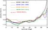 |
Fig. 1 Time average of the logarithmic radial gradient versus target latitude. Black, blue, and orange lines represent each consecutive five year time average of dlnΩ/dlnr obtained from MDI360. The green line shows the same quantity obtained from HMI360. The red dashed line shows the 19 year (1996−2015) time average of dlnΩ/dlnr. The error bars are 1σ. The errors on the orange and blue lines are similar to the black one. The errors on the red dashed line are similar to the thickness of the line. |
4.1. Results obtained from 72-day vs. 360-day data
In this section, we compare the radial gradient derived from splittings obtained from 360-day time series and 72-day time series from both MDI and HMI. First, we show the results of MDI data and then HMI.
The first panel of Fig. 2 shows the 15 year (1996−2011) time average of the radial gradient obtained from data sets MDI360 and MDI72. The result from data set MDI72 is identical to the MDI result found by BSG. For the MDI data, the absolute value of dlnΩ/dlnr is about 5% smaller than the values found by BSG. This difference can be explained by the fact that using MDI360 and HMI360 data sets enables us to probe roughly 3 Mm deeper than using data sets MDI72 and HMI72. As a consequence,  is not linear in r any more, as shown in Fig. 3, which in turn means that the fitted values depend on the modes included.
The maximum value of l = 300 is the same for all data sets, but the minimum value of l is different; see Table 1. Therefore, we compare the results obtained from each set in MDI360 with those from the corresponding five sets of MDI72, using only the common modes. The result is shown in the first panel of Fig. 2. For this comparison we excluded the last data set of MDI72 because it is after the last set in MDI360.
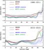 |
Fig. 2 Comparison of time averages of dlnΩ/dlnr versus target latitude using 15 years of MDI data (upper panel) and five years of HMI data (lower panel). In both panels, black and blue lines show results obtained from splittings from 360-day time series of all and common modes (see, Sect. 4.1), respectively. The red and green lines show the results obtained from 72-day time series of all and common modes, respectively. The dotted lines mark the constant values of −0.9 and −1 at all latitudes. The error bars are 1σ. |
 |
Fig. 3
|

Considering only common modes causes us to exclude more than half of the modes from each data set in MDI360 (see last column of Table 1). The difference between the results obtained from MDI360 and MDI72 are reduced substantially and they are now in agreement to better than 1σ up to 50° latitude. This difference increases gradually toward higher latitudes which shows that the results above 50° latitude are not reliable. We note that one would expect the results to be consistent to better than 1σ, as they are obtained from the same underlying data. Thus there is clear evidence that the splitting data suffer from systematic errors.
We applied the same comparison to sets HMI360 and HMI72. The five year time averages from using both all and only the common modes are shown in the bottom panel of Fig. 2. There is a significant discrepancy between the two results obtained from sets HMI360 and HMI72 above 60° latitude which does not disappear even when comparing the results obtained from the common modes. This shows that the HMI data are even more affected by systematic errors than the MDI data.
For HMI data, we carry out further analysis by comparing the results derived from common modes of each year. Except for the first and last year the difference between the results persists. The perfect agreement of the results in the last year encourage us to compare common modes between these two data sets. This comparison shows that the difference between a3 and a5 of those data sets are significant. In average, the values of a3 of HMI360 is larger and a5 is smaller than the corresponding HMI72 ones by about 3σ. There are also clear systematic errors in those coefficients with larger discrepancies in the earlier than in the later years.
Unfortunately, these comparisons do not tell us what causes the systematic errors or how to correct them. Understanding this will require a more detailed analysis (Larson & Schou, in prep.). However, our results suggest that HMI72 suffer from systematic errors as the results obtained using HMI360 are not significantly different from the results of data sets MDI360 and MDI72. Moreover, we expect that the splittings obtained from longer time series have better quality as the peaks are better resolved (Larson & Schou 2015).
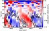 |
Fig. 4 Time variation of dlnΩ/dlnr relative to its 19 year time average. The thin stripe in the plot shows the result obtained from data set 15 overploted on data set 16 as there is 288 days overlap between these two data sets. The contours show the two hemisphere averaged butterfly diagram of the sunspot area of 5 per millionths of a hemisphere (courtesy of D. Hathaway; see http://solarscience.msfc.nasa.gov/greenwch.shtml). |
4.2. Solar cycle variation of the radial gradient
We measure the variation of dlnΩ/dlnr relative to its time averaged value from 1996 to 2015 using data sets MDI360 and HMI360. We show the results in Fig. 4 together with the butterfly diagram. These measurements reveal two cyclic patterns; one at low latitudes from the equator to about 40° latitude and one above 60° latitude. There is no clear signal between about 40° and 60° latitude.
Below 40°, there exist bands where the rotation gradient is about 10% larger and smaller than the average. As illustrated by the butterfly diagram in Fig. 4, the band with steeper than average gradient (blue in Fig. 4) follows the activity belt quite closely. These bands are also similar to the torsional oscillation signal (see, e.g., Howe et al. 2006; Antia et al. 2008).
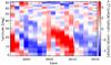 |
Fig. 5 Statistical significance in change of dlnΩ/dlnr relative to its average values at different latitudes and time. σ is the error on dlnΩ/dlnr of each year. |
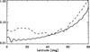 |
Fig. 6 Comparison between the standard deviation of the time variation of the radial shear relative to its time averaged value (dashed line) and the time averaged error of the shear (solid line) obtained from data sets MDI360 and HMI360. |
The temporal variation of dlnΩ/dlnr at high latitudes is more than 10% of its average value and has the opposite behavior to that at low latitudes. However, as we pointed out eirlier the measured values of the gradient above 50° latitude are not reliable, so any results here have to be interpreted with caution.
The statistical significance of these signals is shown in Fig. 5 and the standard deviation in time and the time averaged errors in Fig. 6. The measured signals are statistically significant at low and high latitudes as they are at the 3 to 8σ level, while they are indeed not significant between 40° and 60° latitude.
We note here that the results obtained from MDI360 and HMI360 are only different by about 1% when using modes with  , corresponding roughly to the range used by the 72-day analysis and over which the rotation rate changes linearly with depth.
It is well known that the phase and amplitude of the solar cycle variations of the rotation rate vary with depth and latitude (Vorontsov et al. 2002; Basu & Antia 2003; Howe et al. 2005; Antia et al. 2008), but the temporal variation of the gradient has not been previously reported over the same depth range as used in this work.
Antia et al. (2008) found a similar pattern with similar amplitude of the temporal variation of the radial gradient at 0.98 R⊙ as ours. They used the first eight odd a-coefficients obtained from MDI p and f modes and GONG p modes spanning 1995 to 2007. Despite the similarity in pattern and amplitude, the sign of the change in the gradient of their results is opposite to ours. They saw that sunspots occurred where the absolute value of the gradient is smaller than the average value which is the opposite of what we see. This difference might come from the fact that we are measuring the temporal variation around 0.99 R⊙ while they measured it at 0.98 R⊙. We also note that Antia et al. (2008) used the earlier version of the MDI data (see Larson & Schou 2015 and BSG) which might explain the discrepancy that Antia et al. (2008) saw between GONG and MDI data at 0.98 R⊙ and shallower layers.
5. Conclusion
We make measurements of the radial gradient over 19 years (1996−2015) corresponding to solar cycle 23 and the rising phase of cycle 24 in the outer 13 Mm of the Sun. We use recently available f mode frequency splittings data obtained from 360-day time series of MDI spanning 1996 to 2011 and HMI spanning 2010 to 2015. The values of the radial gradient derived from MDI360 and HMI360 fluctuate between −0.97 and −0.9 up to 50° latitude. These values are a few percent larger than measured values by BSG which are obtained from MDI72 and HMI72. It turns out that this difference comes from the fact that the angular velocity does not change linearly with depth to deeper than about 10 Mm below the surface.
We also compare the radial gradient obtained from common modes of two different data sets of each instrument. These comparisons reveal that the measured values of dlnΩ/dlnr above 50° latitude are not reliable. Another important finding is that there are considerable systematic errors in HMI data that needs further investigation.
By measuring the variation of rotational shear relative to its 19 year time averaged value we find two cyclic patterns at low (0° to 30°) and at high (60° to 80°) latitudes with similar period of the solar cycle. Both patterns show bands of larger and smaller than average shear moving toward the equator and poles at low and high latitudes, respectively. The relative change in the shear is about 10% at low latitudes and 20% at high latitudes. Although the values of dlnΩ/dlnr above 50° are not reliable, the temporal variation of dlnΩ/dlnr is significant above 60° latitudes. This finding may have important implications for dynamo models as this variation is considerable compared to the torsional oscillation (Antia et al. 2008).
The cyclic behavior of the shear at low latitudes agrees with the recent theoretical work by Kitchatinov (2016) who showed that the strength of the shear increases because of the presence of the strong magnetic field. Therefore accurate measurements of the shear might be a way of determining of the sub-surface magnetic field.
Acknowledgments
We thank T. P. Larson for discussions regarding details of the HMI data, and A. Birch for various discussions and his useful comments about the paper. L. Gizon acknowledges support from the Center for Space Science at the NYU Abu Dhabi Institute. SOHO is a project of international cooperation between ESA and NASA. The HMI data are courtesy of NASA/SDO and the HMI science team.
References
- Antia, H. M., Basu, S., & Chitre, S. M. 1998, MNRAS, 298, 543 [NASA ADS] [CrossRef] [Google Scholar]
- Antia, H. M., Basu, S., & Chitre, S. M. 2008, ApJ, 681, 680 [NASA ADS] [CrossRef] [Google Scholar]
- Barekat, A., Schou, J., & Gizon, L. 2014, A&A, 570, L12 [NASA ADS] [CrossRef] [EDP Sciences] [Google Scholar]
- Basu, S., & Antia, H. M. 2003, ApJ, 585, 553 [NASA ADS] [CrossRef] [Google Scholar]
- Brandenburg, A. 2005, ApJ, 625, 539 [Google Scholar]
- Brandenburg, A., & Subramanian, K. 2005, Phys. Rep., 417, 1 [NASA ADS] [CrossRef] [Google Scholar]
- Charbonneau, P. 2010, Liv. Rev. Sol. Phys., 7, 3 [Google Scholar]
- Corbard, T., & Thompson, M. J. 2002, Sol. Phys., 205, 211 [NASA ADS] [CrossRef] [Google Scholar]
- Gizon, L., Birch, A. C., & Spruit, H. C. 2010, ARA&A, 48, 289 [Google Scholar]
- Howe, R. 2009, Liv. Rev. Sol. Phys., 6 [Google Scholar]
- Howe, R., Christensen-Dalsgaard, J., Hill, F., et al. 2005, ApJ, 634, 1405 [NASA ADS] [CrossRef] [Google Scholar]
- Howe, R., Komm, R., Hill, F., et al. 2006, Sol. Phys., 235, 1 [NASA ADS] [CrossRef] [Google Scholar]
- Kitchatinov, L. L. 2016, Astron. Lett., 42, 339 [NASA ADS] [CrossRef] [Google Scholar]
- Kitchatinov, L. L., & Rüdiger, G. 2005, Astron. Nachr., 326, 379 [NASA ADS] [CrossRef] [Google Scholar]
- Küker, M., Arlt, R., & Rüdiger, G. 1999, A&A, 343, 977 [NASA ADS] [Google Scholar]
- Larson, T. P., & Schou, J. 2015, Sol. Phys., 290, 3221 [NASA ADS] [CrossRef] [Google Scholar]
- Scherrer, P. H., Bogart, R. S., Bush, R. I., et al. 1995, Sol. Phys., 162, 129 [Google Scholar]
- Schou, J. 1999, ApJ, 523, L181 [NASA ADS] [CrossRef] [Google Scholar]
- Schou, J., Christensen-Dalsgaard, J., & Thompson, M. J. 1994, ApJ, 433, 389 [NASA ADS] [CrossRef] [Google Scholar]
- Schou, J., Antia, H. M., Basu, S., et al. 1998, ApJ, 505, 390 [NASA ADS] [CrossRef] [Google Scholar]
- Schou, J., Scherrer, P. H., Bush, R. I., et al. 2012, Sol. Phys., 275, 229 [Google Scholar]
- Thompson, M. J., Toomre, J., Anderson, E. R., et al. 1996, Science, 272, 1300 [NASA ADS] [CrossRef] [PubMed] [Google Scholar]
- Vorontsov, S. V., Christensen-Dalsgaard, J., Schou, J., Strakhov, V. N., & Thompson, M. J. 2002, Science, 296, 101 [NASA ADS] [CrossRef] [Google Scholar]
All Tables
All Figures
|
Fig. 1 Time average of the logarithmic radial gradient versus target latitude. Black, blue, and orange lines represent each consecutive five year time average of dlnΩ/dlnr obtained from MDI360. The green line shows the same quantity obtained from HMI360. The red dashed line shows the 19 year (1996−2015) time average of dlnΩ/dlnr. The error bars are 1σ. The errors on the orange and blue lines are similar to the black one. The errors on the red dashed line are similar to the thickness of the line. |
| In the text | |
|
Fig. 2 Comparison of time averages of dlnΩ/dlnr versus target latitude using 15 years of MDI data (upper panel) and five years of HMI data (lower panel). In both panels, black and blue lines show results obtained from splittings from 360-day time series of all and common modes (see, Sect. 4.1), respectively. The red and green lines show the results obtained from 72-day time series of all and common modes, respectively. The dotted lines mark the constant values of −0.9 and −1 at all latitudes. The error bars are 1σ. |
| In the text | |
|
Fig. 3
|
| In the text | |
|
Fig. 4 Time variation of dlnΩ/dlnr relative to its 19 year time average. The thin stripe in the plot shows the result obtained from data set 15 overploted on data set 16 as there is 288 days overlap between these two data sets. The contours show the two hemisphere averaged butterfly diagram of the sunspot area of 5 per millionths of a hemisphere (courtesy of D. Hathaway; see http://solarscience.msfc.nasa.gov/greenwch.shtml). |
| In the text | |
|
Fig. 5 Statistical significance in change of dlnΩ/dlnr relative to its average values at different latitudes and time. σ is the error on dlnΩ/dlnr of each year. |
| In the text | |
|
Fig. 6 Comparison between the standard deviation of the time variation of the radial shear relative to its time averaged value (dashed line) and the time averaged error of the shear (solid line) obtained from data sets MDI360 and HMI360. |
| In the text | |
Current usage metrics show cumulative count of Article Views (full-text article views including HTML views, PDF and ePub downloads, according to the available data) and Abstracts Views on Vision4Press platform.
Data correspond to usage on the plateform after 2015. The current usage metrics is available 48-96 hours after online publication and is updated daily on week days.
Initial download of the metrics may take a while.