| Issue |
A&A
Volume 595, November 2016
|
|
|---|---|---|
| Article Number | A70 | |
| Number of page(s) | 12 | |
| Section | Cosmology (including clusters of galaxies) | |
| DOI | https://doi.org/10.1051/0004-6361/201628567 | |
| Published online | 31 October 2016 | |
Sloan Great Wall as a complex of superclusters with collapsing cores
1 Tartu Observatory, Observatooriumi 1, 61602 Tõravere, Estonia
e-mail: This email address is being protected from spambots. You need JavaScript enabled to view it.
2 Tuorla Observatory, University of Turku, Väisäläntie 20, Piikkiö, Finland
3 Finnish Centre for Astronomy with ESO (FINCA), University of Turku, Väisäläntie 20, Piikkiö, Finland
4 Estonian Academy of Sciences, Kohtu 6, 10130 Tallinn, Estonia
5 ICRANet, Piazza della Repubblica 10, 65122 Pescara, Italy
Received: 21 March 2016
Accepted: 11 August 2016
Abstract
Context. The formation and evolution of the cosmic web is governed by the gravitational attraction of dark matter and antigravity of dark energy (cosmological constant). In the cosmic web, galaxy superclusters or their high-density cores are the largest objects that may collapse at present or during the future evolution.
Aims. We study the dynamical state and possible future evolution of galaxy superclusters from the Sloan Great Wall (SGW), the richest galaxy system in the nearby Universe.
Methods. We calculated supercluster masses using dynamical masses of galaxy groups and stellar masses of galaxies. We employed normal mixture modelling to study the structure of rich SGW superclusters and search for components (cores) in superclusters. We analysed the radial mass distribution in the high-density cores of superclusters centred approximately at rich clusters and used the spherical collapse model to study their dynamical state.
Results. The lower limit of the total mass of the SGW is approximately M = 2.5 × 10¹⁶ h-1 M⊙. Different mass estimators of superclusters agree well, the main uncertainties in masses of superclusters come from missing groups and clusters. We detected three high-density cores in the richest SGW supercluster (SCl 027) and two in the second richest supercluster (SCl 019). They have masses of 1.2 − 5.9 × 10¹⁵ h-1 M⊙ and sizes of up to ≈60 h-1 Mpc. The high-density cores of superclusters are very elongated, flattened perpendicularly to the line of sight. The comparison of the radial mass distribution in the high-density cores with the predictions of spherical collapse model suggests that their central regions with radii smaller than 8 h-1 Mpc and masses of up to M = 2 × 10¹⁵ h-1 M⊙ may be collapsing.
Conclusions. The rich SGW superclusters with their high-density cores represent dynamically evolving environments for studies of the properties of galaxies and galaxy systems.
Key words: large-scale structure of Universe / galaxies: groups: general
© ESO, 2016
1. Introduction
Galaxy superclusters are the largest systems in the complex hierarchical network of galaxies, galaxy groups, clusters, and superclusters (the cosmic web). The structure of the superclusters is formed during a hierarchical evolution where the high-density cores of superclusters are older and dynamically more evolved than outskirts regions. While full rich superclusters are not bound systems, their high-density cores may collapse at present or in the course of the future evolution (Small et al. 1998; Reisenegger et al. 2000; Rines et al. 2002; Nagamine & Loeb 2003; Proust et al. 2006; Dünner et al. 2006; Luparello et al. 2011; Pearson et al. 2014; Chon et al. 2015; O’Mill et al. 2015; Einasto et al. 2015; Gramann et al. 2015). This makes galaxy superclusters unique objects to study their properties and the properties and evolution of the galaxy systems (groups, clusters, and filaments) inside the dynamically evolving environment of superclusters. The size, mass, and other properties of the high-density cores in superclusters give us an information about the largest possibly collapsing objects in the Universe (Lilje & Lahav 1991; Gramann & Suhhonenko 2002; Nagamine & Loeb 2003; Teerikorpi et al. 2015; Lee et al. 2015; Gramann et al. 2015).
The richest nearby galaxy system is the Sloan Great Wall (SGW), discovered in the Sloan Digital Sky Survey (SDSS; Vogeley et al. 2004; Gott et al. 2005), which consists of several rich and poor superclusters (Einasto et al. 2011b). Einasto et al. (2003, 2008) noted that in the core region of the richest supercluster in the SGW (SCl 126 in their study, SCl 027 in Liivamägi et al. 2012, this notation is also used in our study) the concentration of galaxy clusters in a sphere with diameter smaller than 10 h-1 Mpc is very high. This region is a good candidate for a collapsing core of the supercluster. The SGW is not fully covered by the SDSS, its southern extension can be traced by the Las Campanas and 2dF Redshift surveys (Einasto et al. 2003, 2008). The SGW affects the measurements of the topology of the whole SDSS (Park et al. 2005; Saar et al. 2007; Gott et al. 2008). The analysis of rich superclusters in the SGW has shown that they have a different morphology and galaxy and group content (Einasto et al. 2007b, 2010, 2011a,b, 2014). The richest supercluster in the SGW, SCl 027, is one of the most elongated superclusters according to its overall shape (Einasto et al. 2011a). Jaaniste et al. (1998) have noted the flatness of this supercluster; this supercluster is also aligned almost perpendicular to the line of sight. The authors assumed that the flatness of this supercluster is enhanced and we see the effect of the matter inflow towards the supercluster axis, in accordance to what we observe in the nearby space for the Laniakea and Arrowheads superclusters (Tully et al. 2014; Pomarède et al. 2015).
The extreme observed objects like the SGW usually provide tests for theories. For example, while Park et al. (2012) demonstrated that systems with sizes and richness similar to the SGW can be reproduced in the ΛCDM model, Sheth & Diaferio (2011) showed that systems as dense and massive as the SGW may be in tension with the Gaussian initial conditions. Moreover, Einasto et al. (2007b) found that the morphology of the richest supercluster in the SGW is difficult to reproduce with simulations. Einasto et al. (2016) showed that the superclusters from the SGW lie in a wall of a shell-like structure around the rich cluster A1795 in the Bootes supercluster with a radius of about 120 − 130 h-1 Mpc. The pattern of the cosmic web originates from processes in the early Universe. However, it is not yet clear which processes cause shell-like structures in the local cosmic web. This all motivates further studies of the properties of the SGW.
The aim of the present paper is to determine the dynamical, total, and stellar masses of the SGW superclusters, and to analyse the structure of rich SGW superclusters with normal mixture modelling. We compare the mass distribution of the core regions of the superclusters centred at rich galaxy clusters with the predictions of the spherical collapse model, which describes the evolution of a spherically symmetric perturbation in an expanding Universe. The dynamics of a collapsing shell is determined by the mass in its interior. The spherical collapse model has been discussed in detail by Peebles (1980; see also references in Gramann et al. 2015). We estimate the dynamical state and possible future evolution of the core regions of the SGW superclusters and discuss the possibility whether the high-density cores of the SGW superclusters may merge into huge collapsing systems1.
We use the following standard cosmological parameters below: the Hubble parameter H0 = 100 h km s-1 Mpc-1, the matter density Ωm = 0.27, and the dark energy density ΩΛ = 0.73 (Komatsu et al. 2011).
2. Data
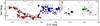 |
Fig. 1 Distribution of galaxy groups in the SGW superclusters in the sky plane in the redshift range 0.04 <z< 0.12. Numbers are order numbers of superclusters in Table 1, and different colours indicate groups in these superclusters. Symbol sizes are proportional to the size of groups in the sky plane. Grey symbols show galaxy groups in other superclusters in this redshift interval. |
We selected data about superclusters and their galaxy and group content from the supercluster and group catalogues by Liivamägi et al. (2012) and Tempel et al. (2012, 2014). These catalogues are based on the MAIN sample of the eighth and tenth data release of the SDSS (Aihara et al. 2011; Ahn et al. 2014) with apparent Galactic extinction-corrected r magnitudes r ≤ 17.77 and redshifts 0.009 ≤ z ≤ 0.200. We corrected the redshifts of galaxies with respect to our motion relative to the CMB and computed the comoving distances of galaxies (see Martínez & Saar 2002; Tempel et al. 2014, for details).
We used the luminosity density field to determine galaxy superclusters. In calculations of the luminosity density field we applied the 1 h-1 Mpc step grid and the B3 spline kernel at the smoothing length 8 h-1 Mpc. While constructing the luminosity density field, we first suppressed the redshift-space distortions (the so-called fingers of God) for groups as explained in Tempel et al. (2014). Connected volumes above a certain density threshold were defined as superclusters. The calculation of the luminosity density field, corrections for the faint galaxies missing from the catalogue, and determination of superclusters are described in detail in Liivamägi et al. (2012).
The luminosity density field is a biased tracer of the underlying mass field, as is shown, for example, by the analysis of the mass-to-light ratios of galaxy systems (Bahcall & Kulier 2014; Einasto et al. 2015). Therefore, in our analysis below we determine the masses of the high-density cores of superclusters as described in Sect. 3.1 and do not directly use the luminosity density field for this purpose.
Einasto et al. (2011b) analysed the properties of the density field superclusters in the region of the SGW at a series of density levels. They concluded that the density level D8 = 5.0 (in units of mean density, ℓmean = 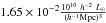 ) is suitable to determine individual superclusters. At this density level superclusters in the SGW form separate systems, and the SGW consists of two rich and three poor superclusters, at lower density levels they join into huge percolating systems together with surrounding superclusters. In our study we use the data about SGW superclusters chosen from the Liivamägi et al. (2012) supercluster catalogue at this density level.
If galaxies were moving solely with the general expansion of the Universe, the redshifts would accurately measure the radial distances of galaxies. Since galaxies have peculiar velocities with respect to the general expansion, their redshift distances are distorted. The galaxy distribution in redshift space is different from that in real space on both small and large scales. On the largest scales, the amplitude of clustering is enhanced as a result of the coherent large-scale velocity field. In contrast to the elongation along the line of sight produced by incoherent velocities within galaxy groups, the galaxy distribution on large scales is flattened along the line of sight (e.g. Kaiser 1987; Gramann et al. 1994; Hamilton 1998,and references therein).
In this paper we use the distribution of galaxies in redshift space. It would, of course, be preferable to define superclusters as in Tully et al. (2014) and Pomarède et al. (2015) considering the real distances of galaxies. Unfortunately, such data for the SGW region are not yet available. Even for the local superclusters, uncertainties are large (Tully et al. 2016). However, we can study the effect of peculiar velocities indirectly and compare the galaxy distribution in the sky plane and in the radial direction. For the richest SGW supercluster, SCl 027, the peculiar velocities may affect its overall shape, and we see the effect of the matter inflow towards the supercluster axis (Jaaniste et al. 1998). In this paper we determine several components in rich SGW superclusters and study their sizes in the sky plane and in the radial direction in more detail.
Data of individual superclusters in the SGW.
Data about galaxy groups in superclusters were taken from the group catalogue by Tempel et al. (2014). The redshift-space distortions (fingers of God) for groups were supressed as described in detail in Tempel et al. (2014). Galaxy groups were determined using the friends-of-friends cluster analysis method introduced in cosmology by Zeldovich et al. (1982) and Huchra & Geller (1982). A galaxy belongs to a group of galaxies if this galaxy has at least one group member galaxy closer than a linking length. In a flux-limited sample the density of galaxies slowly decreases with distance. To take this selection effect properly into account when constructing a group catalogue from a flux-limited sample, the linking length was rescaled with distance, calibrating the scaling relation by observed groups. As a result, the maximum sizes in the sky projection and the velocity dispersions of our groups are similar at all distances. The superclusters lie in a narrow distance interval, therefore we used groups from a flux-limited sample. The details about the data reduction, the group-finding procedure, and the description of the group catalogue can be found in Tempel et al. (2014).
In Table 1 we list the data of the superclusters. The sky distribution of galaxy groups in the region covered by superclusters from the SGW is shown in Fig. 1. The total length of the SGW is approximately 230 h-1 Mpc; without poor superclusters, it is approximately 165 h-1 Mpc. This is comparable with the estimate by Sheth & Diaferio (2011), who found that the diameter of the SGW is about 160 h-1 Mpc. With its length of 230 h-1 Mpc, the SGW is smaller than a recently discovered new member of the Wall family, a very rich supercluster complex called the BOSS Great Wall at a redshift of approximately z = 0.47 (BGW, Lietzen et al. 2016), which has a diameter of about 270 h-1 Mpc. With its huge size and richness, the BGW is an even greater challenge to the cosmological theories than the SGW. In the catalogue of superclusters determined on the basis of X-ray clusters by Chon et al. (2013), the supercluster RXSCJ1305-0221 with its size of about 45 h-1 Mpc corresponds to the part of SCl 027 with Dec < 2°, centred approximately on the rich cluster A1650. The SGW is surrounded by voids. Closer to us, it is located across the void behind the Hercules supercluster with an approximate size of 120 − 140 h-1 Mpc. The distribution of nearby rich superclusters was described in more detail in Einasto et al. (2011a) and in Einasto et al. (2016).
3. Methods
3.1. Masses of superclusters
To calculate the dynamical masses and mass-to-light ratios of superclusters, we used data about the dynamical masses of galaxy groups in superclusters from the catalogue of Tempel et al. (2014). In Fig. 2 we show the dynamical masses of all groups in SGW superclusters. Masses are calculated using the virial theorem, assuming that the galaxy velocity distribution and the Navarro-Frenk-White (NFW, Navarro et al. 1997) projected density profile for galaxy distribution in the plane of the sky are symmetrical. For a detailed description of how the dynamical masses of groups were calculated we refer to Tempel et al. (2014). The masses of poor groups are not well defined, therefore we used the median values of group masses instead of individual masses from Tempel et al. (2014) for groups with Ngal = 2 and 3. To obtain a dynamical mass of a supercluster Mdyn, we summed group dynamical masses. A similar procedure to calculate the dynamical mass of the supercluster was used in Einasto et al. (2015). The reliability of group mass estimation method and mass errors were analysed in Old et al. (2014, 2015), where various mass estimation methods were tested on mock galaxy catalogues. The method used in this work performs reasonably well without a clear bias between true and estimated masses. Since in this paper we are only interested on the masses of superclusters (i.e. we sum over a large number of groups), the statistical uncertainty of an individual group mass estimate is not important. Errors in the supercluster dynamical masses that are due to the group mass errors are estimated to be about 0.3 dex. The supercluster total mass estimates are dominated by systematic biases. Below we discuss some selection effects that may affect mass estimates.
 |
Fig. 2 Dynamical masses of groups vs. group richness for superclusters of the SGW. |
The total masses of superclusters were calculated adding the estimated mass of faint groups and intercluster gas. Each region hosts some single galaxies. They may be the brightest galaxies of faint groups in which other member galaxies are too faint to be observed within SDSS survey magnitude limits (Tempel et al. 2009). We used the median mass of groups with 2 − 3 member galaxies in the SGW superclusters as the mass of these faint groups. To obtain the total mass of these faint groups, this median mass was multiplied with the number of single galaxies. We also added 10% of the total mass as the mass of intercluster gas (see e.g. Pompei et al. 2016). Total masses of superclusters  (here g stands for both groups and gas) were obtained by summing these mass estimates. Approximately 50% of the supercluster total masses comes from groups with at least ten member galaxies, 25% of masses from poor groups with fewer than ten galaxies, and 15% of mass from faint groups presented by single galaxies.
We also calculated total stellar masses of galaxies in superclusters and stellar-to-total mass ratios using data about the stellar masses of supercluster member galaxies from the MPA-JHU spectroscopic catalogue (Tremonti et al. 2004; Brinchmann et al. 2004) in the SDSS CAS database. In this catalogue the different properties of galaxies are obtained by fitting SDSS photometry and spectra with the stellar population synthesis models developed by Bruzual & Charlot (2003). The stellar masses of galaxies are estimated from the galaxy photometry (Kauffmann et al. 2003). The stellar mass of superclusters M∗ is the sum of the stellar masses of galaxies in a supercluster. The stellar-to-total mass ratio M∗/ is the ratio of the stellar mass of galaxies, M∗, and total mass of a supercluster.
In addition, data about stellar masses of the most luminous galaxies in a group can be used to calculate the mass of the haloes to which galaxies belong, employing the relation of stellar mass M* to halo mass Mhalo from Moster et al. (2010), ![Mathematical equation: \begin{equation} \frac{M_{*}}{M_{\mbox{halo}}}=2\left(\frac{M_{*}}{M_{\mbox{halo}}}\right)_0 \left[\left(\frac{M_{\mbox{halo}}}{M_1}\right)^ {-\beta}+\left(\frac{M_{\mbox{halo}}}{M_1}\right)^\gamma\right]^{-1}, \label{eq:stmass} \end{equation}](/articles/aa/full_html/2016/11/aa28567-16/aa28567-16-eq57.png) (1)where (M*/Mhalo)0 = 0.02817 is the normalisation of the stellar to halo mass relation, the halo mass Mhalo is the virial mass of haloes, M1 = 7.925 × 10¹¹ M⊙ is a characteristic mass, and β = 1.068 and γ = 0.611 are the slopes of the low- and high-mass ends of the relation, respectively. This method was used by Lietzen et al. (2016) to estimate the mass of the BGW superclusters. We used this mass estimate for single galaxies and groups of up to nine member galaxies and dynamical masses of groups from the group catalogue of Tempel et al. (2014) for richer groups to calculate a supercluster mass estimate from stellar masses of galaxies
(1)where (M*/Mhalo)0 = 0.02817 is the normalisation of the stellar to halo mass relation, the halo mass Mhalo is the virial mass of haloes, M1 = 7.925 × 10¹¹ M⊙ is a characteristic mass, and β = 1.068 and γ = 0.611 are the slopes of the low- and high-mass ends of the relation, respectively. This method was used by Lietzen et al. (2016) to estimate the mass of the BGW superclusters. We used this mass estimate for single galaxies and groups of up to nine member galaxies and dynamical masses of groups from the group catalogue of Tempel et al. (2014) for richer groups to calculate a supercluster mass estimate from stellar masses of galaxies  . To make this mass estimate comparable to the total mass of superclusters calculated using group dynamical masses, , we also added 10% of the total mass as the mass of gas and denote this mass as
  .
.
3.2. Multidimensional normal mixture modelling
We studied the structure of rich superclusters from the SGW with multidimensional normal mixture modelling, which is based on the analysis of a finite mixture of multivariate Gaussian distributions. Each component in the distribution corresponds to a separate component in the data. For this analysis we employed the Mclust package (Fraley & Raftery 2002; Fraley et al. 2012) in statistical R environment (Ihaka & Gentleman 1996) for the model-based clustering analysis. Mclust searches for an optimal model for the clustering of the data among the models with varying shape, orientation, and volume, and finds the optimal number of components in the data and the membership of components (classification of the data). Mclust also calculates the uncertainty of the classification and determines for each datapoint the probability of belonging to a component. The uncertainty of classification is defined as one minus the highest probability of a datapoint to belong to a component. The mean uncertainty for the full sample is a statistical estimate of the reliability of the results. To study the structure of superclusters, the input data for Mclust were the coordinates of galaxy groups in superclusters. This package has been used, for example, to search for substructure in galaxy groups and clusters and to refine the group-finding algorithm (Einasto et al. 2010, 2012b; Ribeiro et al. 2013; Tempel et al. 2016), to analyse the distribution of different galaxy populations in superclusters (Einasto et al. 2011b), and in morphological classification of superclusters (Einasto et al. 2011a).
Supercluster masses.
3.3. Spherical collapse model
The spherical collapse model describes the evolution of a spherical perturbation in an expanding Universe. This model was studied by Peebles (1980, 1984), Lahav et al. (1991), Eke et al. (1996), and Lokas & Hoffman (2001). In the standard models with cosmological constant, the dark energy started accelerating the expansion at the redshift z ≈ 0.7 and the formation of structure slowed down. At the present epoch, the largest bound structures are just forming. In the future evolution of the Universe, these bound systems separate from each other at an accelerating rate, forming isolated “island Universes” (Chiueh & He 2002; Busha et al. 2003; Dünner et al. 2006).
Chon et al. (2015) and Gramann et al. (2015) analysed the characteristic density contrasts for the turnaround and future collapse in different spherical collapse models. These density contrasts can be used to derive the relations between radius of a perturbation and the interior mass for each essential epoch.
For a spherical volume V = 4πR3/ 3 with radius R the density ratio to the mean density (overdensity) Δρ = ρ/ρm can be calculated as 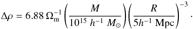 (2)From Eq. (2) we can find the mass of a structure as
  (3)
(3)
Turnaround. One essential moment in the evolution of a spherical perturbation is called turnaround, the moment when the sphere stops expanding together with the Universe and the collapse begins. At the turnaround, the perturbation decouples entirely from the Hubble flow of the homogeneous background. The spherically averaged radial velocity around a system in the shell of radius R can be written as u = HR − vpec, where vH = HR is the Hubble expansion velocity and vpec is the averaged radial peculiar velocity towards the centre of the system. At the turnaround point, the peculiar velocity vpec = HR and u = 0. The peculiar velocity vpec is directly related to the overdensity Δρ. For Ωm = 0.27 and ΩΛ = 0.73 the overdensity at the turnaround point in the spherical collapse model is ΔρT = 13.1 and the mass of a structure at the turnaround point is (Gramann et al. 2015) 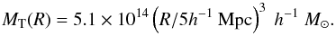 (4)
(4)
Future collapse. The superclusters that have not reached the turnaround at present may eventually turnaround and collapse in the future (Dünner et al. 2006). Chon et al. (2015) showed that for Ωm = 0.27 the overdensity for the future collapse ΔρFC = 8.73, which gives the minimum mass of the structure that will turn around and collapse in the future as 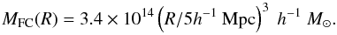 (5)\vspace*{0.8mm}The spherical collapse model has been applied to study, for example, high-density cores in the Corona Borealis supercluster (Small et al. 1998; Pearson et al. 2014), in the Shapley supercluster (Reisenegger et al. 2000; Proust et al. 2006; Chon et al. 2015), in the A2199 supercluster (Rines et al. 2002), and in the A2142 supercluster (Einasto et al. 2015; Gramann et al. 2015).
Below we analyse the structure of superclusters, find their components, and study their masses, sizes, and shapes. We analyse the observed radial mass distribution in components centred on rich galaxy clusters and compare it with the turnaround and future collapse masses predicted by the spherical collapse model.
4. Results
4.1. Masses and mass-to-light ratios of the SGW superclusters
All mass estimates for superclusters are given in Table 2, which shows that for the rich SGW superclusters different mass estimators give quite close values of mass. For the supercluster SCl 019 they are almost identical. The differences between masses from dynamical masses of groups and stellar masses of galaxies are the largest for two poor superclusters, SCl 499 and SCl 1109, where the number of groups is rather low (especially in SCl 1109) and mass estimates have larger scatter. The difference between and comes from the difference of how the group masses are estimated for poor (with fewer than ten member galaxies) groups.
Data of the SCl 027 components.
The main sources of mass uncertainties are several selection effects that may affect the supercluster mass estimates. For example, the SDSS galaxy sample is incomplete because of fibre collisions: the smallest separation between spectroscopic fibres is 55′′, and about 6% of galaxies in the SDSS are without observed spectra. Tempel et al. (2012) studied the effect of missing galaxies on a group catalogue and concluded that this mostly affects galaxy pairs. The authors estimated that approximately 8% of galaxy pairs may be missing from the catalogue. Since they are included as single galaxies and we take them into account as the main galaxies of faint groups, the effect of fibre collisions to our results is minor.
Some galaxy groups and clusters are missing from the supercluster SCl 027 since its southern extension is not covered by SDSS survey. One missing rich cluster is the cluster A1651 (Einasto et al. 2003, 2008). We may assume that the mass of this cluster is of the order of the mass of A1650 with dynamical mass of Mdyn ≈ 0.3 × 10¹⁵ h-1 M⊙. Then the dynamical mass of SCl 027 becomes Mdyn = 10.7 × 10¹⁵ h-1 M⊙, the total mass of SCl 027 is then 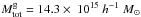 , and the total mass of the SGW is
 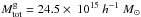 . These masses are lower limits only, since poor groups and single galaxies are also missing from the supercluster.
We used data of the superclusters from the supercluster catalogue with a fixed luminosity density limit, D8 = 5, and may miss lower density outskirts of the superclusters. Our analysis, focused on the high-density cores regions of superclusters, is not affected by this choice, but it may lead to an underestimation of the total masses of superclusters.
Mass-to-light ratios M/L in Table 2 for the rich superclusters and for the full SGW are M/L< 300 h M⊙/L⊙, approximately the same as the mass-to-light ratio of the supercluster A2142 with M/L = 287 h M⊙/L⊙ (Einasto et al. 2015). The values of the mass-to-light ratios for poor superclusters in the SGW depend on the mass estimators that have larger scatter (Table 2) than those for rich superclusters.
4.2. Structure and mass distribution in rich SGW superclusters
To study the structure of the rich SGW superclusters, we searched for possible components (cores) in superclusters with normal mixture modelling. As an input for calculations we used the Cartesian coordinates of galaxy groups in superclusters (including single galaxies), defined as x = d cos δ cos αscl, y = d cos δsinαscl, and z = dsinδ, where d is the comoving distance, αscl = α − αmean is the right ascension (centred on the supercluster mean, αmean), and δ is the declination of the group centre. The angle between the x coordinate and the line of sight is smaller than 5 degrees, so that we can consider x direction as the line-of-sight direction. We analysed the masses, sizes, and shapes of the components. Next we study the group content and radial mass distribution in the cores of rich SGW superclusters centred on rich galaxy clusters and compare it with the predictions of the spherical collapse model.
4.2.1. Supercluster SCl 027
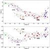 |
Fig. 3 Distribution of galaxy groups in SCl 027 in Cartesian coordinates. Upper panel: yz, and lower panel: yx plane. Filled circles of different colours correspond to galaxy groups from different components. The size of the symbols is proportional to the size of the groups in the sky plane. Ellipses are 1σ covariance ellipses of components as found by normal mixture modelling. Numbers show order numbers of components from Table 3 and Abell numbers of rich clusters in the high-density cores of superclusters. |
Normal mixture modelling with Mclust revealed five components in the supercluster SCl 027. The components were detected with uncertainties of 0.003, which shows that the results of the modelling has very high significance. In Fig. 3 we show the distribution of galaxy groups (including faint groups represented by single galaxies) in different components of SCl 027. In Table 3 we list data about components (the number of groups, masses, sizes, and median luminosity density).
The supercluster SCl 027 has three rich components, approximately centred on rich galaxy clusters (A1650, A1750, and A1773, see Table 3). Each high-density core also hosts other rich galaxy clusters. These compnents have total masses of 2.4 − 5.9 × 10¹⁵ h-1 M⊙ and a largest extent of 30 − 57 h-1 Mpc (Table 3). Their median luminosity density is D8 > 7. The same luminosity density limit was found for the high-density cores of superclusters in Einasto et al. (2007a). These components are the high-density cores of the supercluster.
SCl 027 also has two less massive components with total masses lower than 1.5 × 10¹⁵ h-1 M⊙. Their median luminosity density is D8 ≤ 6. These components form outlying branches of the supercluster. Figure 3 shows that the poor component 4 is probably a combination of two very poor components that coincide in the sky plane (upper panel), but are separated in velocity space (lower panel).
Figure 3 and Table 3 show that the high-density components in SCl 027 are very elongated along the y axis and have a largest extent of 30 − 57 h-1 Mpc. The extent of the components along the x-axis direction (along the line of sight) is 14 − 20 h-1 Mpc. The rich components 1 and 3 lie across the line of sight.
 |
Fig. 4 Mass-radius relation for the high-density cores in the supercluster SCl 027. Violet line shows embedded mass M versus radius of a sphere R for the turnaround T, and dashed grey line for the future collapse FC. The red line shows embedded mass versus radius for the region around the cluster A1650, the blue line shows the region around the cluster A1750, and the green line the region around the cluster A1773. |
Next we analyse the mass distribution in the high-density core regions (components 1, 3, and 5) of SCl 027. We found galaxy groups and single galaxies in the spheres of an increasing radius around rich clusters and calculated the embedded mass. In Fig. 4 we plot the embedded mass M(R) versus radius of a sphere R for these cores of SCl 027 and show the theoretical M − R curves from the spherical collapse model for comparison. According to this model, the radii where the observed mass-radius lines cross the turnaround and future collapse lines correspond to maximum sizes of the regions that may collapse now or in the future. Objects in the area above the turnaround line may have reached the turnaround and are already collapsing, and objects above the future collapse line may collapse in the future. We present in Table 4 the number of galaxy groups and single galaxies in spheres whose radius corresponds to these essential epochs of the collapse together with the embedded masses.
Masses and radii of the central regions of the SCl 027 components.
A1650 region. The central cluster in this region, A1650, is an X-ray cluster (see Einasto et al. 2011a, for details). The rich cluster A1663 also lies in the central region of the component with a distance of 6 h-1 Mpc from A1650. One rich cluster close to this region, the X-ray cluster A1651, lies beyond the SDSS survey declination limits (Einasto et al. 2003, 2008). The mass of the region within the turnaround radius of A1650 may be underestimated because of the mass of this cluster. Assuming that A1651 is a member of this high-density region, the total mass of the region increases approximately by 0.3 × 10¹⁵ h-1 M⊙, and the radius may become approximately 10 h-1 Mpc. In this case, another Abell cluster, A1620, with a mass of 0.4 × 10¹⁵ h-1 M⊙ and at a distance from A1650 of approximately 10 h-1 Mpc, may join the future collapse region around A1650. The total mass of the region within the future collapse radius may then be at least 2.1 × 10¹⁵ h-1 M⊙, which is approximately one-third of the total mass of this high-density core.
A1750 region. The component A1750 forms a separate branch in the supercluster with a length of about 30 h-1 Mpc (Table 3). The richest galaxy cluster here is A1750 with the highest mass of the SGW clusters, approximately 0.8 × 10¹⁵ h-1 M⊙. This is a multicomponent X-ray cluster that shows signs of past merging (Belsole et al. 2004; Einasto et al. 2010, and references therein). The comparison of the radial mass distribution around the cluster A1750 with the predictions of the spherical collapse model shows that the central part of the component with a maximum radius of 8 h-1 Mpc is collapsing or will collapse in the future. Merging events in A1750 may be enhanced by the collapse of the whole region.
A1773 region. The Abell cluster A1773 with a mass of 0.5 × 10¹⁵ h-1 M⊙ is the most massive cluster in this high-density core. The mass distribution around A1773 shows that the region around it within a radius of about 6 h-1 Mpc may be collapsing. Another rich cluster (A1809 with a mass of 0.3 × 10¹⁵ h-1 M⊙) lies at a distance of about 17 h-1 Mpc from A1773 at the edge of the component, beyond the collapsing region.
To summarise, according to the comparison of the mass distribution with the predictions of the spherical collapse model, the central parts of these components in SCl 027 with sizes smaller than 6.5 h-1 Mpc have already reached the turnaround and started to collapse. The sizes of possible future collapse regions do not exceed 8 h-1 Mpc. In this model, collapsing regions are surrounded by regions in the supercluster that will not collapse and continue to expand. The cores in the supercluster are very elongated, with a largest extent of 30 − 57 h-1 Mpc. We may assume that the spherical collapse model only describes the central parts of the possibly collapsing regions, and the actual size of collapsing regions across the line of sight may be larger. The flattened shape of the supercluster cores may be a signature of a possible collapse. However, within collapsing regions and also beyond the turnaround regions the group redshifts are poor indicators of their distance (see also the discussion in Dünner et al. 2007). This affects the estimation of the sizes and masses of the possibly collapsing regions. Dünner et al. (2006) showed that the spherical collapse model applied in real space overestimates the mass of the collapsing structure, and this may lead to the overestimation of the sizes of collapsing regions. The redshift corrections for regions beyond the turnaround region may lead to the underestimation of the sizes of the regions (Dünner et al. 2007). Without knowing the real distances of galaxy groups in the regions it is very difficult to give precise values of the sizes and other parameters of the collapsing regions. This shows the limitations of the spherical collapse model and also the need for correct distances of galaxy groups.
Approximately 60 − 75% of the total mass in (now or in the future) collapsing regions in SCl 027 comes from the mass of galaxy groups with at least ten member galaxies. This is slightly higher than in the full supercluster (50%, see Sect. 3.1). All regions contain single galaxies that represent faint galaxy groups. We found that approximately 6 − 9% of the total mass in the turnaround regions and 12 − 14% of the total mass in the future collapse regions comes from these faint groups, showing that the fraction of single galaxies decreases towards the region centres. This may be due to the selection effect: it is possible that the group-finding algorithm in Tempel et al. (2014) adds single galaxies near rich groups to the clusters. In this case, the masses of the faint groups have been taken into account when calculating the masses of rich groups. During the future evolution, these groups and galaxies may merge with the main cluster of a region, as is shown in the analysis of the future evolution of superclusters from simulations (Araya-Melo et al. 2009). It is therefore also possible that the lower fraction of single galaxies in the turnaround regions is evidence of the merging of single galaxies and poor groups with the main cluster during collapse. When we overestimated the mass of faint groups, these fractions show that errors of masses of the regions due to this are smaller than 10%. The mass-to-light ratios M/L of the collapsing regions are 280 − 300 hM⊙/L⊙, the same as the M/L for the full supercluster.
The ratio of stellar masses to the total mass in the collapsing regions is lower than in the supercluster on average, ≈0.008 − 0.009. This ratio increases towards lower halo masses (Andreon 2010; Bahcall & Kulier 2014; Patel et al. 2015). This may be the reason why this ratio has a lower value in the high-density cores than in the full supercluster.
4.2.2. Supercluster SCl 019
In SCl 019 the analysis with Mclust identified six components. The uncertainty of the classification is 0.004, showing that the components in the supercluster have been found with very high significance. The distribution of galaxy groups (including faint groups represented by single galaxies) in the components is shown in Fig. 5. Table 5 presents the number of groups, masses, and sizes of supercluster components.
Two components in SCl 019 have a median luminosity density of D8 ≥ 7, they are the high-density cores of the supercluster. The total mass in these components is 1.2 − 3.2 × 10¹⁵ h-1 M⊙, which means that it is less massive than the most massive high-density cores in SCl 027. The richest, most elongated, and highest mass component in SCl 019 is centred on the group Gr5278 (first component in Table 5). This group corresponds to the Zwicky cluster, Zw1215.1+0400 (Zwicky et al. 1961). The first component also hosts another rich cluster, A1516. The largest extent of this component is ≈65 h-1 Mpc. Another rich component (2) in SCl 019 hosts two rich groups, one of them in galaxy cluster A1424.
Four components in SCl 019 have median densities D8 < 7, they are poorer and with total masses lower than 1 × 10¹⁵ h-1 M⊙. Comparison of Figs. 3 and 5 shows that the components in SCl 019 have a higher variety of shapes and orientations (in the sky distribution) than those in SCl 027. Components are flattened along the line of sight.
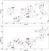 |
Fig. 5 Distribution of galaxy groups in SCl 019 in Cartesian coordinates. Upper panel: yz, and lower panel: yx plane. Filled circles of different colours correspond to galaxy groups from different components. The size of the symbols is proportional to the size of groups in the sky plane. Ellipses are 1σ covariance ellipses of components as found by normal mixture modelling. Numbers show order numbers of components from Table 5 and numbers of rich clusters in the high-density cores of the supercluster. |
Data of the SCl 019 components.
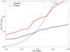 |
Fig. 6 Mass-radius relation for the high-density cores in the supercluster SCl 019. Violet line shows the embedded mass M versus radius of a sphere R for the turnaround T, and the dashed grey line shows the future collapse FC. The red line shows the embedded mass versus radius for the region around the cluster Gr5278, the blue line shows the region around the cluster A1424. |
Next we analyse the group content and mass distribution around the rich galaxy clusters Gr5278 and A1424 in the high-density cores of SCl 019 and compare it with the predictions of the spherical collapse model (Fig. 6 and Table 6).
Gr5278 region. Two rich clusters, Gr5278 with a mass of 0.6 × 10¹⁵ h-1 M⊙ and A1516 with a mass of 0.4 × 10¹⁵ h-1 M⊙ lie in this region. They are both X-ray clusters (Popesso et al. 2007; Piffaretti et al. 2011). The cluster Gr5278 is the richest and most massive cluster in SCl 019. Comparison with the spherical collapse model shows that the size of the possible (now or in the future) collapsing region is smaller than 10 h-1 Mpc, as we found also for the supercluster SCl 027.
The mass-to light ratio of the central region of the component is higher than for the full supercluster, ≈350 hM⊙/L⊙, because of the very massive cluster in the region. The fraction of single galaxies in the turnaround region is 8%, and in the future collapse region 12%.
A1424 region. This component is separated from the Gr5278 component by a small underdense region. The cluster A1424 is located at the outskirts of the component, but since this cluster is the most massive cluster in the component, we analysed the mass distribution around it. Table 6 and Fig. 6 suggest that the region around the cluster A1424 with a mass of about 0.8 × 10¹⁵ h-1 M⊙ and a radius of about 6 h-1 Mpc may be collapsing. The radius of the future collapse region is about 7 h-1 Mpc.
In the A1424 region the fraction of single galaxies in both the turnaround and the future collapse regions is approximately 12%. In SCl 019 60 − 75% of the total mass in (now or in the future) collapsing regions comes from galaxy groups with at least ten member galaxies. In the Gr5278 region this fraction is the highest, 75%. In this supercluster the fraction of the total mass that comes from faint groups represented by single galaxies also decreases towards the region centres.
4.2.3. Poor superclusters from the SGW
Masses and radii of the central regions of the SCl 019 components.
Poor superclusters from the SGW are listed in Tables 1 and 2. The poor supercluster SCl 499 with its two X-ray clusters (A1205 and A1238) corresponds to the X-ray supercluster RXSCJ1116+0206 in the catalogue of Chon et al. (2013). The superclusters SCl 499 and SCl 1109 are very elongated, and we only studied the mass distribution in SCl 319. We calculated masses in spheres of increasing radii centred on the cluster A1066 with a mass of about 0.4 × 10¹⁵ h-1 M⊙. We found that the region that embeds three rich galaxy groups and has a total mass of 0.69 × 10¹⁵ h-1 M⊙ and a radius of 5 h-1 Mpc may have reached the turnaround and started to collapse. The region with a total mass of 0.74 × 10¹⁵ h-1 M⊙ and a radius of R ≈ 6.5 h-1 Mpc (and perhaps the whole supercluster SCl 319) will collapse in the future.
5. Discussion and summary
Masses of the SGW superclusters. We calculated the masses of the SGW superclusters using the dynamical masses of galaxy groups as one mass estimate, and the stellar masses of the main galaxies in groups to obtain the masses of galaxy groups as another mass estimate. The stellar masses of the main galaxies of groups have previously been used to determine the mass of the BOSS Great Wall superclusters (Lietzen et al. 2016). This approach is especially promising in cases when the mass estimates of galaxy groups in superclusters are not available, like in distant superclusters.
We found that the two mass estimators agree well. The main uncertainty of supercluster masses comes from missing groups and clusters, and from the mass estimate of faint groups. The bias between the masses of superclusters determined using group masses and the total mass of the supercluster have been studied from simulations (Chon et al. 2014). They showed that the bias between masses depends on the richness of groups; it is lower when low-mass groups are used to construct the supercluster catalogues. We found that the bias factor (the ratio of the dynamical mass of the supercluster and the total mass of the supercluster) is of about 1.4, which agrees well with results reported by Chon et al. (2014) based on simulations, considering that they used higher mass groups to determine superclusters. This is also similar to what Einasto et al. (2015) found for the supercluster A2142.
The masses of the SGW superclusters and their high-density core regions are in the mass range of other observed superclusters of average richness (see e.g. Johnston-Hollitt et al. 2008; Schirmer et al. 2011; Pompei et al. 2016; Einasto et al. 2015). They are lower than the masses of very rich superclusters such as the Shapley supercluster, the Corona Borealis supercluster, and other very rich superclusters (Reisenegger et al. 2000; Proust et al. 2006; Ragone et al. 2006; Pearson et al. 2014; O’Mill et al. 2015). The mass-to-light ratios of the SGW superclusters, M/L ≈ 300 h M⊙/L⊙, are close to the values of the mass-to-light ratios for other rich superclusters (Gavazzi et al. 2004; Schirmer et al. 2011; Einasto et al. 2015). Moreover, the components in rich SGW superclusters have masses that are comparable to the masses of simulated superclusters of average richness (Chon et al. 2014; Araya-Melo et al. 2009). The masses of rich SGW superclusters are of the same order as the high end of simulated supercluster masses.
The total volume and mass of the SGW were estimated in Sheth & Diaferio (2011). The authors obtained that the volume of the SGW is 7.2 × 10⁵ (h-1 Mpc)3, the effective radius 55 h-1 Mpc, and the total mass of the SGW is 1.2 × 10¹⁷ h-1 M⊙. These values are higher than we obtained, the difference comes from the different way of estimating the volume and mass of the supercluster. Sheth & Diaferio (2011) assumed that the shape of the SGW can be approximated with a sphere, which led to overestimation of the volume and mass of the SGW in comparison with our study. We found that the effective radius of the full SGW (radius of a sphere with the volume of the SGW) is approximately 22 h-1 Mpc, significantly smaller than estimated by Sheth & Diaferio (2011).
Mass distribution in the high-density cores of superclusters. We analysed the radial mass distribution in the high-density cores of rich SGW superclusters centred on rich galaxy clusters and compared it with the predictions of the spherical collapse model. This comparison showed that the central regions of the components with radii up to approximately 6 − 7 h-1 Mpc may be collapsing now or in the future. This limit corresponds to the size of the shortest axis of very elongated regions, the size of possibly collapsing regions along the longest axes of systems may be larger. The analysis of the correlations between velocities of galaxy clusters from simulations showed that up to separations of 10 h-1 Mpc clusters approach each other and their attraction dominates the bulk motions (Cen et al. 1994). This agrees well with the minimum size of possibly collapsing regions in supercluster components.
The collapsing high-density cores have been studied in the Shapley and the Corona Borealis superclusters (Reisenegger et al. 2000; Pearson et al. 2014; Chon et al. 2015), in the Perseus-Pisces supercluster (Hanski et al. 2001; Teerikorpi et al. 2015), in the A2199 supercluster, the member of the Hercules supercluster (Einasto et al. 2001; Rines et al. 2002), in the SC0028-0005 supercluster (O’Mill et al. 2015), and in the A2142 supercluster (Einasto et al. 2015; Gramann et al. 2015). In these studies several methods were used to estimate the size and mass of the collapsing regions, based on overdensity criteria and dynamical criteria (see e.g. Reisenegger et al. 2000; Dünner et al. 2007; Chon et al. 2015). Comparison of the methods shows that radii of the collapsing regions obtained with different methods agree well (Reisenegger et al. 2000; Pearson et al. 2014; Chon et al. 2015). These studies have shown that the sizes of collapsing cores of superclusters typically do not exceed approximately 10 h-1 Mpc, which is also what we found for the central regions of the SGW supercluster components. According to Reisenegger et al. (2000) and Pearson et al. (2014), very massive collapsing cores with a number of rich galaxy clusters in the Shapley supercluster and in the Corona Borealis supercluster are larger and more massive. Pearson et al. (2014) noted that the collapsing core in the Corona Borealis supercluster has this size only if there is a reasonable amount of intercluster mass. Full very rich and massive superclusters are not bound systems (Chon et al. 2013, 2015), as also suggested in our study of the SGW superclusters. Individual components in the SGW superclusters may form separate superclusters in the future.
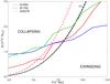 |
Fig. 7 Mass-radius relation for two Ωm values. The red line denotes the turnaround T and the black line denotes the future collapse FC. The dashed lines correspond to Ωm = 0.3 and the solid lines to Ωm = 0.27. Other lines denote high-density cores in SCl 027 and SCl 019, as shown in the plot. |
The mutual distances between the component centres in the supercluster SCl 027 are approximately 35 h-1 Mpc and 50 h-1 Mpc, and in the supercluster SCl 019 approximately 20 h-1 Mpc. Numerical simulations show that the positions of the high-density peaks in the galaxy distribution in the early Universe are fixed by the processes during or just after the inflation and do not change much during the cosmic evolution, only the amplitude of over- and underdensities grows with time (Kofman & Shandarin 1988; Bond et al. 1996; van de Weygaert & Schaap 2009; Suhhonenko et al. 2011, and references therein). Observational data of the movements of galaxies in the nearby Laniakea and Arrowhead superclusters show that galaxy velocities are directed towards supercluster axis (Tully et al. 2014; Pomarède et al. 2015), and galaxies are moving from underdense regions towards high-density regions. This process may accelerate the collapse of individual cores, but it is unlikely that the cores will approach each other and merge.
Several studies have shown that the values of the overdensity for turnaround and future collapse only weakly depend on the exact value of ΩΛ and change only slightly with matter density Ωm (Lilje & Lahav 1991; Chon et al. 2015; Gramann et al. 2015). For example, for Ωm = 0.27, as adopted in the present paper, the overdensity for the turnaround ΔρT = 13.1, and for Ωm = 0.3 (Planck Collaboration XIII 2015), ΔρT = 12.2 (Gramann et al. 2015). In Fig. 7 we show the mass-radius relation for Ωm = 0.27 and Ωm = 0.3 together with the radial mass distribution in the SGW superclusters. The differences between overdensity values for various Ωm values are much smaller than the uncertainties of the mass estimates of supercluster high-density core regions (for overdensity values see the tables in Chon et al. 2015; Gramann et al. 2015). Therefore it is questionable to apply the turnaround as a cosmological test in supercluster scales, as proposed, for example, by Pavlidou & Tomaras (2014). More precise mass estimates for a larger number of supercluster (cores) are needed for this.
The structure of rich SGW superclusters and supercluster morphology. Normal mixture modelling showed that the richest SGW superclusters consist of a number of components. The richest components hosts rich galaxy clusters; they are the high-density cores of superclusters. Components are very elongated in the sky distribution, their short axes point along the line of sight. This may be due to their real shape, but the flatness of supercluster components may also be enhanced by the large-scale velocity field (Kaiser 1987; Gramann et al. 1994).
The distribution of components in superclusters reflects the overall morphology of superclusters. In SCl 027 the components lie along the main body of the supercluster described as being of filament morphology (Einasto et al. 2011a). SCl 019 was described morphologically as having a rich and complex inner structure with many galaxy chains connecting galaxy clusters in the supercluster (spider-type morphology; Einasto et al. 2011a). This is reflected in the much less regular distribution of the components in SCl 019 in comparison with SCl 027. Earlier studies have shown that the morphology of superclusters and the properties of galaxies and groups in them are related. Superclusters of filament morphology host a higher fraction of red passive galaxies than the superclusters of spider morphology, where the galaxy groups also have a higher amount of substructure (Einasto et al. 2012a, 2014). These differences may be related with the dynamical state of the superclusters and galaxy groups in them, spider-type superclusters being dynamically younger and more active than filament-type superclusters. The detailed study of the properties of galaxies and galaxy groups in the richest SGW superclusters and their high-density cores may give us an insight into their dynamical state.
We summarise the main results as follows:
We determined the masses of the SGW superclusters using dynamical masses of groups and stellar masses of the main galaxies in groups, and found a good agreement between mass estimates. The lower limit of the total mass of the SGW is approximately M = 2.5 × 10¹⁶ h-1 M⊙.
We applied normal mixture modelling to study the structure of superclusters and identify their high-density cores. This is a new and promising approach to study the structure of superclusters and detect their high-density cores.
The richest SGW superclusters consists of several very elongated high-density cores with masses of the richest components of up to 6 × 10¹⁵ h-1 M⊙ and sizes of up to 65 h-1 Mpc. Their short axes lie approximately along the line of sight, and their sizes are typically smaller then 20 h-1 Mpc.
The core regions of the components with radii smaller than 8 h-1 Mpc may already be collapsing. This is probably only the shortest size of the collapsing regions.
The study of the properties of galaxies and galaxy groups in different regions in superclusters may provide information about environmental effects that shape the galaxy properties in superclusters, and about the regions themselves. We plan to continue the study of the dynamical state of galaxy superclusters from observations and simulations, as well as the properties of galaxies and their systems (groups, clusters, and filaments) in dynamically evolving environment of superclusters.
At http://www.aai.ee/~maret/SGW.html we present online an interactive 3D model that shows the distribution of galaxy groups in the superclusters from the SGW.
Acknowledgments
We thank the referee for valuable comments and suggestions.
We are pleased to thank the SDSS Team for the publicly available data releases. Funding for the Sloan Digital Sky Survey (SDSS) and SDSS-II has been provided by the Alfred P. Sloan Foundation, the Participating Institutions, the National Science Foundation, the US Department of Energy, the National Aeronautics and Space Administration, the Japanese Monbukagakusho, and the Max Planck Society, and the Higher Education Funding Council for England. The SDSS Web site is http://www.sdss.org/. The SDSS is managed by the Astrophysical Research Consortium (ARC) for the Participating Institutions. The Participating Institutions are the American Museum of Natural History, Astrophysical Institute Potsdam, University of Basel, University of Cambridge, Case Western Reserve University, The University of Chicago, Drexel University, Fermilab, the Institute for Advanced Study, the Japan Participation Group, Johns Hopkins University, the Joint Institute for Nuclear Astrophysics, the Kavli Institute for Particle Astrophysics and Cosmology, the Korean Scientist Group, the Chinese Academy of Sciences (LAMOST), Los Alamos National Laboratory, the Max-Planck-Institute for Astronomy (MPIA), the Max-Planck-Institute for Astrophysics (MPA), New Mexico State University, Ohio State University, University of Pittsburgh, University of Portsmouth, Princeton University, the United States Naval Observatory, and the University of Washington. In this work we used R statistical environment (Ihaka & Gentleman 1996). We acknowledge the support by the Estonian Research Council grants IUT26-2, IUT40-2, and by the Centre of Excellence “Dark side of the Universe” (TK133) financed by the European Union through the European Regional Development Fund, and by ICRAnet through a professorship for Jaan Einasto. HL is supported by Turku University Foundation.
References
- Ahn, C. P., Alexandroff, R., Allen de Prieto, C., et al. 2014, ApJS, 211, 17 [NASA ADS] [CrossRef] [Google Scholar]
- Aihara, H., Allen de Prieto, C., An, D., et al. 2011, ApJS, 193, 29 [NASA ADS] [CrossRef] [Google Scholar]
- Andreon, S. 2010, MNRAS, 407, 263 [NASA ADS] [CrossRef] [Google Scholar]
- Araya-Melo, P. A., Reisenegger, A., Meza, A., et al. 2009, MNRAS, 399, 97 [Google Scholar]
- Bahcall, N. A., & Kulier, A. 2014, MNRAS, 439, 2505 [NASA ADS] [CrossRef] [Google Scholar]
- Belsole, E., Pratt, G. W., Sauvageot, J.-L., & Bourdin, H. 2004, A&A, 415, 821 [NASA ADS] [CrossRef] [EDP Sciences] [Google Scholar]
- Bond, J. R., Kofman, L., & Pogosyan, D. 1996, Nature, 380, 603 [NASA ADS] [CrossRef] [Google Scholar]
- Brinchmann, J., Charlot, S., White, S. D. M., et al. 2004, MNRAS, 351, 1151 [NASA ADS] [CrossRef] [Google Scholar]
- Bruzual, G., & Charlot, S. 2003, MNRAS, 344, 1000 [NASA ADS] [CrossRef] [Google Scholar]
- Busha, M. T., Adams, F. C., Wechsler, R. H., & Evrard, A. E. 2003, ApJ, 596, 713 [NASA ADS] [CrossRef] [Google Scholar]
- Cen, R., Bahcall, N. A., & Gramann, M. 1994, ApJ, 437, L51 [NASA ADS] [CrossRef] [Google Scholar]
- Chiueh, T., & He, X.-G. 2002, Phys. Rev. D, 65, 123 [Google Scholar]
- Chon, G., Böhringer, H., & Nowak, N. 2013, MNRAS, 429, 3272 [NASA ADS] [CrossRef] [Google Scholar]
- Chon, G., Böhringer, H., Collins, C. A., & Krause, M. 2014, A&A, 567, A144 [NASA ADS] [CrossRef] [EDP Sciences] [Google Scholar]
- Chon, G., Böhringer, H., & Zaroubi, S. 2015, A&A, 575, L14 [NASA ADS] [CrossRef] [EDP Sciences] [Google Scholar]
- Dünner, R., Araya, P. A., Meza, A., & Reisenegger, A. 2006, MNRAS, 366, 803 [NASA ADS] [CrossRef] [Google Scholar]
- Dünner, R., Reisenegger, A., Meza, A., Araya, P. A., & Quintana, H. 2007, MNRAS, 376, 1577 [NASA ADS] [CrossRef] [Google Scholar]
- Einasto, M., Einasto, J., Tago, E., Müller, V., & Andernach, H. 2001, AJ, 122, 2222 [CrossRef] [Google Scholar]
- Einasto, M., Jaaniste, J., Einasto, J., et al. 2003, A&A, 405, 821 [NASA ADS] [CrossRef] [EDP Sciences] [Google Scholar]
- Einasto, M., Einasto, J., Tago, E., et al. 2007a, A&A, 464, 815 [NASA ADS] [CrossRef] [EDP Sciences] [Google Scholar]
- Einasto, M., Saar, E., Liivamägi, L. J., et al. 2007b, A&A, 476, 697 [NASA ADS] [CrossRef] [EDP Sciences] [Google Scholar]
- Einasto, M., Saar, E., Martínez, V. J., et al. 2008, ApJ, 685, 83 [NASA ADS] [CrossRef] [Google Scholar]
- Einasto, M., Tago, E., Saar, E., et al. 2010, A&A, 522, A92 [NASA ADS] [CrossRef] [EDP Sciences] [Google Scholar]
- Einasto, M., Liivamägi, L. J., Tago, E., et al. 2011a, A&A, 532, A5 [NASA ADS] [CrossRef] [EDP Sciences] [Google Scholar]
- Einasto, M., Liivamägi, L. J., Tempel, E., et al. 2011b, ApJ, 736, 51 [NASA ADS] [CrossRef] [Google Scholar]
- Einasto, M., Liivamägi, L. J., Tempel, E., et al. 2012a, A&A, 542, A36 [NASA ADS] [CrossRef] [EDP Sciences] [Google Scholar]
- Einasto, M., Gramann, M., Saar, E., et al. 2015, A&A, 580, A69 [NASA ADS] [CrossRef] [EDP Sciences] [Google Scholar]
- Einasto, M., Lietzen, H., Tempel, E., et al. 2014, A&A, 562, A87 [NASA ADS] [CrossRef] [EDP Sciences] [Google Scholar]
- Einasto, M., Heinämäki, P., Liivamägi, L. J., et al. 2016, A&A, 587, A116 [NASA ADS] [CrossRef] [EDP Sciences] [Google Scholar]
- Einasto, M., Vennik, J., Nurmi, P., et al. 2012b, A&A, 540, A123 [NASA ADS] [CrossRef] [EDP Sciences] [Google Scholar]
- Eke, V. R., Cole, S., & Frenk, C. S. 1996, MNRAS, 282, 263 [NASA ADS] [CrossRef] [Google Scholar]
- Fraley, C., & Raftery, A. E. 2002, J. Amer. Stat. Assoc., 97, 611 [Google Scholar]
- Fraley, C., Raftery, A. E., Murphy, T. B., & Scrucca, L. 2012, mclust Version 4 for Normal Mixture Modeling for Model-Based Clustering, Classification, and Density Estimation [Google Scholar]
- Gavazzi, R., Mellier, Y., Fort, B., Cuillandre, J.-C., & Dantel-Fort, M. 2004, A&A, 422, 407 [NASA ADS] [CrossRef] [EDP Sciences] [Google Scholar]
- Gott,III, J. R., Jurić, M., Schlegel, D., et al. 2005, ApJ, 624, 463 [NASA ADS] [CrossRef] [Google Scholar]
- Gott,III, J. R., Hambrick, D. C., Vogeley, M. S., et al. 2008, ApJ, 675, 16 [NASA ADS] [CrossRef] [Google Scholar]
- Gramann, M., & Suhhonenko, I. 2002, MNRAS, 337, 1417 [NASA ADS] [CrossRef] [Google Scholar]
- Gramann, M., Cen, R., & Gott, III, J. R. 1994, ApJ, 425, 382 [NASA ADS] [CrossRef] [Google Scholar]
- Gramann, M., Einasto, M., Heinämäki, P., et al. 2015, A&A, 581, A135 [NASA ADS] [CrossRef] [EDP Sciences] [Google Scholar]
- Hamilton, A. J. S. 1998, in The Evolving Universe, ed. D. Hamilton, Astrophys. Space Sci. Libr., 231, 185 [NASA ADS] [CrossRef] [Google Scholar]
- Hanski, M. O., Theureau, G., Ekholm, T., & Teerikorpi, P. 2001, A&A, 378, 345 [NASA ADS] [CrossRef] [EDP Sciences] [Google Scholar]
- Huchra, J. P., & Geller, M. J. 1982, ApJ, 257, 423 [NASA ADS] [CrossRef] [Google Scholar]
- Ihaka, R., & Gentleman, R. 1996, J. Computational and Graphical Statistics, 5, 299 [Google Scholar]
- Jaaniste, J., Tago, E., Einasto, M., et al. 1998, A&A, 336, 35 [NASA ADS] [Google Scholar]
- Johnston-Hollitt, M., Sato, M., Gill, J. A., Fleenor, M. C., & Brick, A.-M. 2008, MNRAS, 390, 289 [NASA ADS] [CrossRef] [Google Scholar]
- Kaiser, N. 1987, MNRAS, 227, 1 [NASA ADS] [CrossRef] [Google Scholar]
- Kauffmann, G., Heckman, T. M., White, S. D. M., et al. 2003, MNRAS, 341, 33 [NASA ADS] [CrossRef] [Google Scholar]
- Kofman, L. A., & Shandarin, S. F. 1988, Nature, 334, 129 [NASA ADS] [CrossRef] [Google Scholar]
- Komatsu, E., Smith, K. M., Dunkley, J., et al. 2011, ApJS, 192, 18 [NASA ADS] [CrossRef] [Google Scholar]
- Lahav, O., Lilje, P. B., Primack, J. R., & Rees, M. J. 1991, MNRAS, 251, 128 [NASA ADS] [CrossRef] [Google Scholar]
- Lee, J., Kim, S., & Rey, S.-C. 2015, ApJ, 815, 43 [NASA ADS] [CrossRef] [Google Scholar]
- Lietzen, H., Tempel, E., Liivamägi, L. J., et al. 2016, A&A, 588, L4 [NASA ADS] [CrossRef] [EDP Sciences] [Google Scholar]
- Liivamägi, L. J., Tempel, E., & Saar, E. 2012, A&A, 539, A80 [NASA ADS] [CrossRef] [EDP Sciences] [Google Scholar]
- Lilje, P. B., & Lahav, O. 1991, ApJ, 374, 29 [NASA ADS] [CrossRef] [Google Scholar]
- Lokas, E. L., & Hoffman, Y. 2001, in Identification of Dark Matter, eds. N. J. C. Spooner, & V. Kudryavtsev (World Scientific Publ.), 121 [Google Scholar]
- Luparello, H., Lares, M., Lambas, D. G., & Padilla, N. 2011, MNRAS, 415, 964 [NASA ADS] [CrossRef] [Google Scholar]
- Martínez, V. J., & Saar, E. 2002, Statistics of the Galaxy Distribution, Proc. of Conf. (Boca Raton: Chapman & Hall/CRC) [Google Scholar]
- Moster, B. P., Somerville, R. S., Maulbetsch, C., et al. 2010, ApJ, 710, 903 [NASA ADS] [CrossRef] [Google Scholar]
- Nagamine, K., & Loeb, A. 2003, New A, 8, 439 [NASA ADS] [CrossRef] [Google Scholar]
- Navarro, J. F., Frenk, C. S., & White, S. D. M. 1997, ApJ, 490, 493 [NASA ADS] [CrossRef] [Google Scholar]
- Old, L., Skibba, R. A., Pearce, F. R., et al. 2014, MNRAS, 441, 1513 [NASA ADS] [CrossRef] [Google Scholar]
- Old, L., Wojtak, R., Mamon, G. A., et al. 2015, MNRAS, 449, 1897 [NASA ADS] [CrossRef] [Google Scholar]
- O’Mill, A. L., Proust, D., Capelato, H. V., et al. 2015, MNRAS, 453, 868 [NASA ADS] [CrossRef] [Google Scholar]
- Park, C., Choi, Y.-Y., Vogeley, M. S., et al. 2005, ApJ, 633, 11 [NASA ADS] [CrossRef] [Google Scholar]
- Park, C., Choi, Y.-Y., Kim, J., et al. 2012, ApJ, 759, L7 [NASA ADS] [CrossRef] [Google Scholar]
- Patel, S. G., Kelson, D. D., Williams, R. J., et al. 2015, ApJ, 799, L17 [NASA ADS] [CrossRef] [Google Scholar]
- Pavlidou, V., & Tomaras, T. N. 2014, J. Cosmology Astropart. Phys., 9, 020 [Google Scholar]
- Pearson, D. W., Batiste, M., & Batuski, D. J. 2014, MNRAS, 441, 1601 [NASA ADS] [CrossRef] [Google Scholar]
- Peebles, P. J. E. 1980, The large-scale structure of the Universe (Princeton University Press) [Google Scholar]
- Peebles, P. J. E. 1984, ApJ, 284, 439 [NASA ADS] [CrossRef] [Google Scholar]
- Piffaretti, R., Arnaud, M., Pratt, G. W., Pointecouteau, E., & Melin, J.-B. 2011, A&A, 534, A109 [NASA ADS] [CrossRef] [EDP Sciences] [Google Scholar]
- Planck Collaboration XIII. 2016, A&A, 594, A13 [NASA ADS] [CrossRef] [EDP Sciences] [Google Scholar]
- Pomarède, D., Tully, R. B., Hoffman, Y., & Courtois, H. M. 2015, ApJ, 812, 17 [NASA ADS] [CrossRef] [Google Scholar]
- Pompei, E., Adami, C., Eckert, D., et al. 2016, A&A, 592, A6 [NASA ADS] [CrossRef] [EDP Sciences] [Google Scholar]
- Popesso, P., Biviano, A., Böhringer, H., & Romaniello, M. 2007, A&A, 461, 397 [NASA ADS] [CrossRef] [EDP Sciences] [Google Scholar]
- Proust, D., Quintana, H., Carrasco, E. R., et al. 2006, A&A, 447, 133 [NASA ADS] [CrossRef] [EDP Sciences] [Google Scholar]
- Ragone, C. J., Muriel, H., Proust, D., Reisenegger, A., & Quintana, H. 2006, A&A, 445, 819 [NASA ADS] [CrossRef] [EDP Sciences] [Google Scholar]
- Reisenegger, A., Quintana, H., Carrasco, E. R., & Maze, J. 2000, AJ, 120, 523 [Google Scholar]
- Ribeiro, A. L. B., de Carvalho, R. R., Trevisan, M., et al. 2013, MNRAS, 434, 784 [NASA ADS] [CrossRef] [Google Scholar]
- Rines, K., Geller, M. J., Diaferio, A., et al. 2002, AJ, 124, 1266 [NASA ADS] [CrossRef] [Google Scholar]
- Saar, E., Martínez, V. J., Starck, J.-L., & Donoho, D. L. 2007, MNRAS, 374, 1030 [NASA ADS] [CrossRef] [Google Scholar]
- Schirmer, M., Hildebrandt, H., Kuijken, K., & Erben, T. 2011, A&A, 532, A57 [NASA ADS] [CrossRef] [EDP Sciences] [Google Scholar]
- Sheth, R. K., & Diaferio, A. 2011, MNRAS, 417, 2938 [Google Scholar]
- Small, T. A., Ma, C.-P., Sargent, W. L. W., & Hamilton, D. 1998, ApJ, 492, 45 [NASA ADS] [CrossRef] [Google Scholar]
- Suhhonenko, I., Einasto, J., Liivamägi, L. J., et al. 2011, A&A, 531, A149 [NASA ADS] [CrossRef] [EDP Sciences] [Google Scholar]
- Teerikorpi, P., Heinämäki, P., Nurmi, P., et al. 2015, A&A, 577, A144 [NASA ADS] [CrossRef] [EDP Sciences] [Google Scholar]
- Tempel, E., Einasto, J., Einasto, M., Saar, E., & Tago, E. 2009, A&A, 495, 37 [NASA ADS] [CrossRef] [EDP Sciences] [Google Scholar]
- Tempel, E., Tago, E., & Liivamägi, L. J. 2012, A&A, 540, A106 [NASA ADS] [CrossRef] [EDP Sciences] [Google Scholar]
- Tempel, E., Tamm, A., Gramann, M., et al. 2014, A&A, 566, A1 [NASA ADS] [CrossRef] [EDP Sciences] [Google Scholar]
- Tempel, E., Kipper, R., Tamm, A., et al. 2016, A&A, 588, A14 [NASA ADS] [CrossRef] [EDP Sciences] [Google Scholar]
- Tremonti, C. A., Heckman, T. M., Kauffmann, G., et al. 2004, ApJ, 613, 898 [NASA ADS] [CrossRef] [Google Scholar]
- Tully, R. B., Courtois, H., Hoffman, Y., & Pomarède, D. 2014, Nature, 513, 71 [NASA ADS] [CrossRef] [Google Scholar]
- Tully, R. B., Courtois, H. M., & Sorce, J. G. 2016, AJ, 152, 50 [NASA ADS] [CrossRef] [Google Scholar]
- van de Weygaert, R., & Schaap, W. 2009, in Data Analysis in Cosmology, , eds. V. J. Martínez, E. Saar, E. Martínez-González, & M.-J. Pons-Bordería, Lect. Notes Phys. (Berlin: Springer Verlag), 291, 665 [Google Scholar]
- Vogeley, M. S., Hoyle, F., Rojas, R. R., & Goldberg, D. M. 2004, in Outskirts of Galaxy Clusters: Intense Life in the Suburbs, ed. A. Diaferio, IAU Colloq., 195, 5 [Google Scholar]
- Zeldovich, I. B., Einasto, J., & Shandarin, S. F. 1982, Nature, 300, 407 [NASA ADS] [CrossRef] [Google Scholar]
- Zwicky, F., Herzog, E., Wild, P., Karpowicz, M., & Kowal, C. T. 1961, Catalogue of galaxies and of clusters of galaxies, Vol. I (California Institute of Technology (CIT)) [Google Scholar]
All Tables
All Figures
|
Fig. 1 Distribution of galaxy groups in the SGW superclusters in the sky plane in the redshift range 0.04 <z< 0.12. Numbers are order numbers of superclusters in Table 1, and different colours indicate groups in these superclusters. Symbol sizes are proportional to the size of groups in the sky plane. Grey symbols show galaxy groups in other superclusters in this redshift interval. |
| In the text | |
|
Fig. 2 Dynamical masses of groups vs. group richness for superclusters of the SGW. |
| In the text | |
|
Fig. 3 Distribution of galaxy groups in SCl 027 in Cartesian coordinates. Upper panel: yz, and lower panel: yx plane. Filled circles of different colours correspond to galaxy groups from different components. The size of the symbols is proportional to the size of the groups in the sky plane. Ellipses are 1σ covariance ellipses of components as found by normal mixture modelling. Numbers show order numbers of components from Table 3 and Abell numbers of rich clusters in the high-density cores of superclusters. |
| In the text | |
|
Fig. 4 Mass-radius relation for the high-density cores in the supercluster SCl 027. Violet line shows embedded mass M versus radius of a sphere R for the turnaround T, and dashed grey line for the future collapse FC. The red line shows embedded mass versus radius for the region around the cluster A1650, the blue line shows the region around the cluster A1750, and the green line the region around the cluster A1773. |
| In the text | |
|
Fig. 5 Distribution of galaxy groups in SCl 019 in Cartesian coordinates. Upper panel: yz, and lower panel: yx plane. Filled circles of different colours correspond to galaxy groups from different components. The size of the symbols is proportional to the size of groups in the sky plane. Ellipses are 1σ covariance ellipses of components as found by normal mixture modelling. Numbers show order numbers of components from Table 5 and numbers of rich clusters in the high-density cores of the supercluster. |
| In the text | |
|
Fig. 6 Mass-radius relation for the high-density cores in the supercluster SCl 019. Violet line shows the embedded mass M versus radius of a sphere R for the turnaround T, and the dashed grey line shows the future collapse FC. The red line shows the embedded mass versus radius for the region around the cluster Gr5278, the blue line shows the region around the cluster A1424. |
| In the text | |
|
Fig. 7 Mass-radius relation for two Ωm values. The red line denotes the turnaround T and the black line denotes the future collapse FC. The dashed lines correspond to Ωm = 0.3 and the solid lines to Ωm = 0.27. Other lines denote high-density cores in SCl 027 and SCl 019, as shown in the plot. |
| In the text | |
Current usage metrics show cumulative count of Article Views (full-text article views including HTML views, PDF and ePub downloads, according to the available data) and Abstracts Views on Vision4Press platform.
Data correspond to usage on the plateform after 2015. The current usage metrics is available 48-96 hours after online publication and is updated daily on week days.
Initial download of the metrics may take a while.