| Issue |
A&A
Volume 595, November 2016
|
|
|---|---|---|
| Article Number | A43 | |
| Number of page(s) | 22 | |
| Section | Extragalactic astronomy | |
| DOI | https://doi.org/10.1051/0004-6361/201628139 | |
| Published online | 26 October 2016 | |
Dust properties in H II regions in M 33⋆
1 Dept. Física Teórica y del Cosmos, Universidad de Granada, 18010 Granada, Spain
e-mail: This email address is being protected from spambots. You need JavaScript enabled to view it.
2 Instituto Universitario Carlos I de Física Teórica y Computacional, Universidad de Granada, 18071 Granada, Spain
3 Institute of Astronomy, University of Cambridge, Madingley Road, Cambridge, CB3 0HA, UK
4 Instituto Radioastronomía Milimétrica, Av. Divina Pastora 7, Núcleo Central, 18012 Granada, Spain
5 Unidad de Astronomía, Fac. Cs. Básicas, Universidad de Antofagasta, 02800 Avda. U. de Antofagasta, Antofagasta, Chile
6 Argelander-Institut für Astronomie, University of Bonn, Auf dem Hügel 71, 53121 Bonn, Germany
7 Univ. Bordeaux, Laboratoire d’Astrophysique de Bordeaux, CNRS, LAB, UMR 5804, 33270 Floirac, France
8 Instituto de Astrofísica de Andalucía – CSIC. Apdo. 3004, 18008 Granada, Spain
9 Department of Physics and Astronomy, University College London, Gower Street, London WC1E 6BT, UK
10 Sterrenkundig Observatorium, Universiteit Gent, Krijgslaan 281 S9, 9000 Gent, Belgium
11 Institute of Astronomy and Astrophysics, National Observatory of Athens, P. Penteli, 15236 Athens, Greece
12 Department of Astronomy, University of Minnesota, 116 Church St. SE, Minneapolis, MN 55414, USA
13 NASA Goddard Space Flight Center, Code 665, Greenbelt, MD 20771, USA
14 Department of Physics & Astronomy, Johns Hopkins University, Baltimore, MD, 21218, USA
Received: 15 January 2016
Accepted: 10 June 2016
Abstract
Context. The infrared emission (IR) of the interstellar dust has been claimed to be a tracer of the star formation rate. However, the conversion of the IR emission into star formation rate can be strongly dependent on the physical properties of the dust, which are affected by the environmental conditions where the dust is embedded.
Aims. We study here the dust properties of a set of H ii regions in the Local Group galaxy M 33 presenting different spatial configurations between the stars, gas, and dust to understand the dust evolution in different environments.
Methods. We modelled the spectral energy distribution (SED) of each region using the DustEM tool and obtained the mass relative to hydrogen for very small grains (VSG, YVSG), polycyclic aromatic hydrocarbons (YPAH), and big grains (BG, YBG). We furthermore performed a pixel-by-pixel SED modelling and derived maps of the relative mass of each grain type for the whole surface of the two most luminous H ii regions in M 33, NGC 604 and NGC 595.
Results. The relative mass of the VSGs (YVSG/YTOTAL) changes with the morphology of the region: YVSG/YTOTAL is a factor of ~1.7 higher for H ii regions classified as filled and mixed than for regions presenting a shell structure. The enhancement in VSGs within NGC 604 and NGC 595 is correlated to expansive gas structures with velocities ≥50 km s-1. The gas-to-dust ratio derived for the H ii regions in our sample exhibits two regimes related to the H i−H2 transition of the interstellar medium (ISM). Regions corresponding to the H i diffuse regime present a gas-to-dust ratio compatible with the expected value if we assume that the gas-to-dust ratio scales linearly with metallicity, while regions corresponding to a H2 molecular phase present a flatter dust-gas surface density distribution.
Conclusions. The fraction of VSGs can be affected by the conditions of the interstellar environment: strong shocks of ~50–90 km s-1 existing in the interior of the most luminous H ii regions can lead to fragmentation of BGs into smaller ones, while the more evolved shell and clear shell objects provide a more quiescent environment where reformation of dust BGs might occur. The gas-to-dust variations found in this analysis might imply that grain coagulation and/or gas-phase metal incorporation into the dust mass is occurring in the interior of the H ii regions in M 33.
Key words: galaxies: individual: M 33 / galaxies: ISM / Hiiregions / ISM: bubbles / dust, extinction / infrared: ISM
Full Tables A.1 and A.2 are only available at the CDS via anonymous ftp to cdsarc.u-strasbg.fr (130.79.128.5) or via http://cdsarc.u-strasbg.fr/viz-bin/qcat?J/A+A/595/A43
© ESO, 2016
1. Introduction
The presence of interstellar dust in star-forming regions is supported by the observed mid-infrared (MIR) and far-infrared (FIR) emission in star-forming regions. In the Milky Way several studies have shown that dust is ubiquitous in star-forming regions and at the same time exhibits a wide range of properties (see e.g. Churchwell et al. 2009). Within a single galaxy the properties of dust emission change very strongly, from cold dust in the diffuse interstellar medium (ISM) to warm dust processed by the intense radiation field within the star-forming regions (Xilouris et al. 2012). Since the pioneer study of Calzetti et al. (2005), where a correlation between the 24 μm emission and the emission of the ionised gas was observed for star-forming regions in NGC 5194, several studies have probed the correlation between the IR dust emission and the emission of ionised gas in many galaxies with different properties (see e.g. Calzetti et al. 2007). Dust appears to survive in the interior of the star-forming regions, and its infrared emission is spatially correlated with the location of the newly formed stars.
Interstellar dust can also be affected by the environment in which it is located and thus exhibits different physical properties depending on the characteristics of the ISM that surrounds it. Dust does not remain with the same physical properties during its lifetime, as dust particles interact with the medium in which they are embedded (see Jones 2004). Dust is a key for understanding star formation, its production and destruction mechanisms, and how these mechanisms are linked to star formation is not completely clear as yet. This hampers our ability to accurately trace star formation or the gas reservoir, as this requires assumptions on the dust properties and size distribution.
Several mechanisms affect the evolution of the dust, some of them leading to a change in the physical properties and others to the destruction of a particular dust species (see Jones 2004, for a review). (i) Photon-grain interactions: high-energy UV-visible photons are absorbed and scattered, leading to grain heating and subsequent thermal emission. (ii) Atom- or ion-grain interactions: at high gas temperature, impinging atoms or ions can erode the grain and lead to sputtering of atoms from the grain. This mechanism depends on the relative gas-grain velocities. When the gas-grain velocity is due to the motion of the grain relative to the gas, as in a supernova (SN) shock wave, the process is called non-thermal sputtering; and if the relative gas-grain velocity is due to the thermal velocity of the gas ions (e.g. in a hot gas at more than 105 K as it occurs in the hot post-shock gas in a SN bubble), the process is called thermal sputtering. In general, sputtering affects the grain surfaces but cannot disrupt the grain cores unless complete grain destructions occurs. (iii) Low-energy grain-grain collisions lead to grain coagulation, increasing the mean grain size, while at higher energies grain fragmentation or disruption can occur. Shattering in grain-grain collisions preserves the total grain mass, but alters the grain size distribution.
Jones et al. (1996; see also Bocchio et al. 2014, for dust processing with the new dust model from Jones et al. 2013) studied the effects of grain shattering in shocks through grain-grain collisions that produce fragmentation of all, or part of, a grain into smaller but distinct sub-grains. The result is a transfer of mass from large (~200 Å) grains into smaller (~60 Å) ones, which leads to a change of the grain size distribution – the mass percentage of small grains formed by shattering is up to 40% higher for grains with radii greater than 50 Å.
Despite the theoretical studies regarding the dust evolution within different environments, little has been done from the observational point of view. Recently, Paradis et al. (2011) and Stephens et al. (2014; see also Compiègne et al. 2008) have presented evidence of dust evolution for some H ii regions in the Large Magellanic Cloud (LMC). Furthermore, Bernard et al. (2008) found a 70 μm excess in the spectral energy distribution (SED) of the LMC with respect to the Milky Way and proposed the production of a large fraction of very small grains (VSGs) through erosion of larger grains as the most plausible explanation for this excess.
Although these studies show evidence of a change in the dust size distribution of individual H ii regions, a systematic study of a large H ii region sample covering a wide range of physical properties is needed to firmly conclude about the evolution of dust in different environments. Relaño et al. (2013, hereafter Paper I)presented observational SEDs of a set of H ii regions in the nearby (840 kpc, Freedman et al. 1991) spiral galaxy M 33 covering a wavelength range from the UV (GALEX) to the FIR (Herschel). Using the Hα emission distribution of each object, the regions of the sample were classified as filled, mixed, shell and clear shell objects (Fig. 2 in Paper I, shows examples of each type). Each morphological classification might well represent an evolutionary stage of the H ii region from ages of a few Myr for filled and mixed regions, where gas (and dust) is co-spatial with the stellar cluster, to 5–10 Myr for shells and clear shells, where the massive stellar winds and SN have created holes and shell structures around the stellar cluster (Whitmore et al. 2011). A different star-gas-dust spatial configuration (see Fig. 3 in Verley et al. 2010) is also expected for each morphological type. Paper I studied trends in the observed SEDs with the morphology of the region and found that the FIR SED peak of regions with shell morphology seems to be located towards longer wavelengths, implying that the dust is cooler for this type of objects. Assuming a characteristic environment for each H ii region type (the star-gas-dust spatial configuration is different in filled compact regions and shell-like objects), we would expect an evolution of the physical properties of the dust in each morphological type.
Dust evolution processes can be studied through the variation of the dust size distribution and, in particular, with the ratio of the abundance of small to large grains (Compiègne et al. 2008). Therefore, we present a study of the relative abundance of small to large grains for the H ii regions in M 33 and analyse the results in terms of the region morphology. We estimate the abundances of the different grain types by modelling the observed SEDs with the dust emission tool DustEM (Compiègne et al. 2011). DustEM allows us to obtain the mass abundance relative to hydrogen of each dust grain population included in the model (several dust models can be considered by the software tool), as well as the intensity of the interstellar radiation field (ISRF) heating the dust.
The paper is organised as follows. In Sect. 2 we present the observations and describe in detail the new data set that complements the SEDs that have been published in Paper I. In Sect. 3 we describe how the observed SEDs were derived and how the dust modelling is performed. The results are described in Sect. 4. A detailed analysis of the two most luminous H ii regions in M 33, NGC 604 and NGC 595, is presented in Sect. 5. Finally, in Sect. 6 we summarise the main conclusions of this paper.
2. Data
The observed SEDs of the H ii regions were built up using data from the FUV to FIR wavelength range. We used the same UV, Hα, Spitzer data as presented in Paper I, therefore we refer to this paper for a more detailed description of these particular data. Here, we describe the new data set that we included in this study.
2.1. Herschel data
In Paper I we used 100 μm and 160 μm PACS and 250 μm SPIRE data. For this paper, we used the latest version of 100 μm PACS data reprocessed with Scanamorphos v16 (Roussel 2013) as described in Boquien et al. (2011) with a resolution of 7.̋7, and the new observed 70 μm and 160 μm PACS data, obtained in a follow-up open-time cycle 2 programme of Herschel (Boquien et al. 2015) with a resolution of 5.̋5 and 11.̋2. We took the difference of the astrometry into account in the 100 μm image that has been reported in Boquien et al. (2015) and changed the coordinates of the image accordingly. The field of view of the new 70 μm and 160 μm PACS data is slightly smaller than the field of view of the data set in Paper I, and four regions of the original sample in Paper I are missing in the new PACS images. Therefore, the 70 μm and 160 μm fluxes of these regions were discarded from the analysis presented here.
The SPIRE and the 100 μm PACS data were taken in the framework of the HerM33es open-time key project (Kramer et al. 2010). The 250 μm SPIRE image with a resolution of 21.̋2 was obtained using the new version 10.3.0 of the Herschel data processing system (HIPE, Ott 2010, 2011). For a description of the data reduction we refer to Xilouris et al. (2012). The calibration uncertainties are 5% for the PACS images and 15% for the 250 μm SPIRE image. Owing to the low spatial resolution we did not use 350 μm and 500 μm SPIRE data.
2.2. WISE data
The Wide-field Infrared Survey Explorer (WISE; Wright et al. 2010) observed M 33 in four photometric bands: 3.4 μm (W1), 4.6 μm (W2), 12 μm (W3), and 22 μm (W4) with spatial resolutions of 6.̋1, 6.̋4, 6.̋5, and 12.̋0, respectively. We used the image mosaic service Montage1 to obtain the final mosaic image of M 33 in each band. After subtracting the global background, the WISE maps were converted from digital numbers into Jy using the photometric zero points given in Table 1 of the Explanatory Supplement to the WISE All-Sky Data Release Products2. We followed Jarrett et al. (2013) and applied the corrections recommended by them for extended source photometry. First, we applied an aperture correction that accounts for the point spread function (PSF) profile fitting used in the WISE absolute photometric calibration. The corrections are 0.034, 0.041, –0.030, and 0.029 mag for the W1, W2, W3, and W4 bands, respectively. The second correction is a colour correction that we did not apply here, as it is already taken into account by the SED fitting process within the DustEM code (see Sect. 3.2). The third correction, related to a discrepancy in the calibration between the WISE photometric standard blue stars and red galaxies, only applies to the W4 image and accounts for a factor of 0.92. The calibration accuracy of the WISE maps are 2.4%, 2.8%, 4.5%, and 5.7%, for W1, W2, W3, and W4 images (Jarrett et al. 2011).
2.3. LABOCA 870 μm data
The Large APEX BOlometer CAmera (LABOCA) is a multi-channel bolometer array for continuum observations (Siringo et al. 2009) installed at the Atacama Pathfinder Experiment (APEX3) telescope covering a bandwidth of ~150 μm around the central wavelength of 870 μm. The FWHM of the PSF is ~19.̋2 (Weiß et al. 2009), close to that of the 250 μm SPIRE band. We refer to Hermelo et al. (2016) for a description of the data reduction of the LABOCA observations of M 33. Ten H ii regions of the original sample in Paper I are located close to the edge of the LABOCA field of view and thus we were not able to perform an accurate photometry for these objects. Therefore, their fluxes in this band were not considered in the analysis of the SEDs. The uncertainty in the calibration is ~12%.
Observed LABOCA fluxes include emission from the CO rotational transition CO(3-2) at 870 μm and from thermal free-free emission. Hermelo et al. (2016) estimated the CO(3-2) contribution to the total LABOCA flux of M 33 to be ~7.6%. We adopted this value for the fluxes of the individual H ii regions. The thermal emission was estimated from the analysis of Tabatabaei et al. (2007) at 3.6 cm. These authors obtained a thermal fraction of 76.4% and 99.2% for the observed 3.6 cm flux from multi-wavelength data with two different methods. Adopting the mean value of both methods and a spectral index of 0.1, we obtain a thermal contribution of 3% to the LABOCA observed flux. We took CO(3-2) and thermal contributions into account and subtracted them from the observed LABOCA fluxes for each object.
2.4. GISMO 2 mm data of NGC 604
The Goddard-IRAM Superconducting 2 Millimeter Observer (GISMO) continuum camera on the IRAM 30 m telescope (Staguhn et al. 2006) works at a central frequency of 150 GHz, with Δν/ν = 0.15 (or a band-width of 22 GHz at 150 GHz). It comprises an array of 8 × 16 pixels separated by 14′′ on the sky, with a resolution of 17.5′′.
Observations of NGC 604 were conducted in several shifts, in April 2012, and April, October, and November 2013, during about 26 h of total observing time by 181 on-the-fly scanning maps in total power of 10′ × 10′ in size. Typical scanning speeds were 44′′/s. To correct for atmospheric transmission, the IRAM taumeter was used, which continuously measures the sky opacity at 225 GHz. The GISMO conversion factor, 29.3 counts/Jy, was derived from Mars, Uranus, and Neptune observations. The relative calibration uncertainty is estimated to be ~10% (see the reports on the GISMO performance4). To obtain the positions of the GISMO pixels on the sky and source gains, Mars was mapped covering the source within each pixel. The crush5 data processing software (version 2.16-3; Kovacs 2008) was used with the options for faint emission. NGC 604 is detected with a total flux density of 64.4 mJy integrated over a 74.2′′ aperture radii. The peak flux density is 18 mJy/beam. The rms was measured to be 0.55 mJy/beam. The final map of NGC 604 is presented in Fig. 1.
The observed GISMO flux needs to be corrected for the thermal emission of the free electrons within the ionised gas. We used the results from Tabatabaei et al. (2007) at 3.6 cm to estimate this contribution as in Sect. 2.3. We obtained that 51% of the observed flux in GISMO corresponds to thermal emission. We subtracted this contribution from the observed GISMO flux for the global and the pixel-by-pixel analysis presented in Sect. 5.
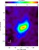 |
Fig. 1 2 mm image of NGC 604 observed with the GISMO continuum camera. The final spatial resolution of the image is 21.0′′ to match the other data. |
2.5. CO and HI data
We used here the 12CO(J = 2–1) (at 230.538 GHz) velocity-integrated intensity map presented in Druard et al. (2014). The spatial resolution of the map is 12′′ with a pixel size of 3′′. The HI (21 cm) intensity map is presented in Gratier et al. (2010), it has a spatial resolution of 17′′ and a pixel size of 4.5′′. Details of the data reduction are given in Druard et al. (2014) and Gratier et al. (2010) for CO and HI intensity maps, respectively.
3. Method
In this section we explain how the photometry was performed and describe the SED fitting procedure.
3.1. Photometry
We aim to model the SED of the set of H ii regions studied in Paper I including the new PACS, WISE, and LABOCA data. Since we also use the new version of the SPIRE 250 μm data, we smoothed and registered all the images from the FUV to LABOCA, CO, and HI to the resolution of the new version of the SPIRE 250 μm image. The final data set has a spatial resolution (FWHM) of 21.2′′ (~86 pc) and a pixel size of 6′′ (~24 pc).
The total flux for each region was obtained using the IRAF task phot and the central coordinates and aperture radii defined in Table 1 of Paper I. The photometric aperture radii range from ~50 pc for filled regions to ~250 pc for clear shell objects (see Fig. 4 in Paper I). The local background was defined and subtracted as in Paper I. Regions with absolute fluxes lower than their errors were assigned an upper limit of three times the estimated uncertainty in the flux. The negative fluxes showing absolute values higher than the corresponding errors were discarded from the study. The final fluxes for all the bands used in this paper, as well as FUV, NUV and Hα fluxes, are given in Tables A.1 and A.2.
We compared the fluxes obtained here from the updated data set with the fluxes already published in Paper I. For FUV, NUV, IRAC, and MIPS bands we find differences of ≤20% mainly related to the subtraction of the local background (differences for the fluxes without subtracting the local background are ~1%). The lower the flux of the region, the larger the difference, which shows that for some regions the uncertainties are dominated by the estimate of the local background.
For the PACS 100 μm and 160 μm images the differences in the fluxes are larger. The main reason is that there is a significant difference in the data reduction process of the last version (Scanamorphos v16) of these images, improving the drift removal (Boquien et al. 2015). This can affect the fluxes for the low-luminosity H ii regions in these bands (see Fig. B.1).
3.2. SED modelling
To study the properties of the dust in the sample of H ii regions, we fitted the observed SEDs with the dust emission tool DustEM (Compiègne et al. 2011). The code allows a combination of various grain types as input and gives the emissivity per hydrogen atom (NH = NHI + 2NH2) for each grain type based on the incident radiation field strength and the grain physics in the optically thin limit. The free parameters are the mass relative to hydrogen of each dust population (Yi), the intensity of a NIR continuum modelled using a black body with a temperature of 1000 K, and the ISRF parameter G0, which is the scale factor to the solar neighbourhood ISRF given in Mathis et al. (1983). The origin of the 1000 K black body emission is uncertain. It was observed by Lu et al. (2003) with ISO/ISOPHOT in a sample of 45 normal star-forming galaxies, it has also been observed in the spectra of reflection nebulae (Sellgren et al. 1983) and in the diffuse cirrus emission of the Milky Way (Flagey et al. 2006). We were unable to fit the SEDs of our regions without this component, therefore we included it and obtained the scale factor as an output parameter. Given an observed SED and the associated uncertainties, DustEM performs the SED fitting using the MPFIT IDL minimisation routine (Markwardt 2009), based on the Levenberg-Marquardt minimisation method. In the process DustEM predicts the SED values that would be observed by the astronomical instruments taking the colour corrections for wide filters and the flux conventions used by the instruments into account.
DustEM can handle an arbitrary number of grain types and size distributions. We adopted here the Compiègne et al. (2011) dust model (Compiegne dust model), which includes three dust components: polycyclic aromatic hydrocarbons (PAHs) with radii r ≲ 10 Å, hydrogenated amorphous carbonaceus grains (amC), and amorphous silicates (aSil) with radii r ≳ 100 Å. The population of amorphous carbon dust is divided into small (SamC, r ~ 10−100 Å) and large (LamC, r ≳ 100 Å) grains. In addition, the model distinguishes between ionised and neutral PAHs. We define YVSG = YSamC and YBG = YLamC + YaSil in a similar way as in Flagey et al. (2011). In the fitting process we kept the ratio between the aSil and LamC grains at the constant value given by the model, 5.38, to maintain an acceptable ratio between observational data points and input parameters. We compared the results of this dust model with the classical one proposed by Desert et al. (1990; hereafter the Desert dust model), which consists of three dust grain types: PAHs, VSGs of carbonaceous material, and big grains (BGs) of astronomical silicates. The comparison is presented in Appendix C. In general, the SED is also well fitted with the Desert dust model, except for the 6–9 μm wavelength range where the model underpredicts the observed emission. This shows that the Desert dust model might not be reliable in constraining the PAH abundance.
3.3. Input radiation field
A more realistic ISRF for a typical H ii region compared to the ISRF from Mathis et al. (1983) used as default in DustEM is that of a young star cluster. We generated the spectrum of a young star cluster of 4 Myr using the online STARBURST99 application (Leitherer et al. 1999). We assumed a Kroupa initial mass function (IMF; Kroupa 2001) and Geneva stellar tracks and obtained the spectrum for a fixed stellar mass of 104 M⊙ and 4 Myr age. The stellar mass and the age are consistent with those expected from the Hα and FUV luminosities of the brightest H ii regions in M 33 (see Fig. 5 of Relaño & Kennicutt 2009). In Fig. 2 we show the 4 Myr (continuous line) and Mathis (dashed line) ISRFs. A 4 Myr ISRF is harder and contributes significantly to the UV part of the spectrum.
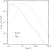 |
Fig. 2 Comparison of Mathis et al. (1983) ISRF (dashed line) and an ISRF of a 4 Myr star cluster (continuous line; see text for details). Both ISRFs have been scaled to the same maximum intensity for a better comparison. The ISRF of a 4 Myr star cluster has a significant contribution in the UV part of the spectrum. |
The different shapes of the two ISRFs can influence the heating of the different types of dust grains. In Fig. 3 we show the results of the DustEM modelling for both ISRFs. YVSG does not change significantly when a different ISRF is assumed, and YBG changes, but the change is small and marginally located within the data dispersion. However, YPAH and the scale of the ISRF do change for Mathis and 4 Myr star cluster ISRFs. YPAH for the Mathis ISRF is about 3 times higher than YPAH when a 4 Myr star cluster ISRF is assumed, and G0 is about60 times higher than F0, where F0 is defined in the same way as G0 but for the 4 Myr star cluster ISRF.
The change in the scale parameter of the ISRF intensity is expected, as the 4 Myr star cluster ISRF is harder than that of Mathis. The YPAH is higher for the Mathis ISRF because of the ISRF shape. For the Compiegne dust model we expect, following the extinction curve given in Compiègne et al. (2011), that the PAHs will absorb more radiation in the UV part of the spectrum than in the optical. Thus, for a 4 Myr star cluster ISRF, which has a significant component in the UV wavelength range, the amount of PAH grains needed to explain the emission in the 3–10 μm range of the observed SED will be lower than the one required for the Mathis ISRF. This shows that unless we are able to characterise the shape of the ISRF heating the dust within the regions we are not able to constrain the PAH abundance completely, there is a degeneracy between the PAH abundance and the scaling factor of the ISRF. However, we are able to infer conclusions on the YPAH distribution within the region, as we show in Sect. 5. In the following we use a 4 Myr star cluster ISRF to model the SEDs of our H ii region sample.
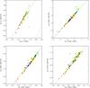 |
Fig. 3 Comparison of the DustEM output parameters for the H ii regions in our sample using a 4 Myr star cluster ISRF and a Mathis ISRF. Top left: scale factor of the ISRF intensity, top right: YVSG, bottom left: YBG, and bottom right: YPAH. The continuous line corresponds to the linear fit to the data and the dashed line is the one-to-one relation. The colour code corresponds to the morphology of the region classified in Paper I: blue circles are filled regions, green squares mixed ones, and red triangles shells or clear shells. |
4. Statistical analysis of H ii regions
4.1. Results of the modelling
In Fig. 4 we show some examples of SEDs modelled with the DustEM code. The PAH emission dominates the SED at shorter wavelengths (3–12 μm), while the emission of the VSGs is highest between 24 μm and 100 μm. At longer wavelengths (λ> 100 μm), the SED is dominated by the emission of the BGs. All the SEDs are fitted with residuals lower than ~50% (see the bottom part of each figure).
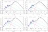 |
Fig. 4 Example of SED models for four regions of the sample catalogued as filled (top left), mixed (top right), shell (bottom left), and clear shell (bottom right). These regions correspond to regions 5, 98, 45, and 78 in Table B.1 in Paper I, respectively. Region 98 is the most luminous H ii region in M 33, NGC 604. The best-fit SED (continuous black line) is obtained assuming a 4 Myr star cluster ISRF and Compiegne dust model. Light blue points: observed data with the errors, red squares: modelled broad-band fluxes, dashed-dot blue line: total (ionised and neutral) PAH emission, dashed-dot green line: VSG (SamC) grain emission, dashed-dot red line: BG (LamC and aSil grains) emission, and dashed purple line: NIR continuum. |
In Fig. 5 we analyse the relative dust masses for each grain type for the best fit with a 4 Myr cluster ISRF. In the lower panels we plot the dust masses of the BGs and the PAHs relative to the total dust abundance for the best fit. BGs represent the highest dust mass fraction in the regions (~90%, and varying within a small range) independently of the morphological type. The relative mass of the PAHs is ≲5% except for three objects. Draine & Li (2007) found a value of 4.6% for the relative mass of the PAHs in the Milky Way and Galliano et al. (2008) showed that the PAH fraction varies significantly with the metallicity. The relative mass of the PAHs found here for most of our objects is consistent with the trend presented in Fig. 25 of Galliano et al. (2008) considering the metallicity of M 33, ZM33 ~ 0.5 Z⊙ (due to the shallow metallicity gradient (Bresolin 2011), we use a mean value between the extreme cases of the radial gradient as the characteristic metallicity for M 33). There are no variations with morphology, but we observe a trend of lower YPAH/YTOTAL for regions with high FUV flux. We show here that the relative PAH mass abundance obtained using a 4 Myr cluster ISRF and the Desert dust model (see Fig. C.1) is lower than the one predicted by the Compiegne dust model.
Statistics of YVSG/YTOTAL, YPAH/YTOTAL, and YBG/YTOTAL for each morphological type of the H ii regions in our sample.
The top right panel of Fig. 5 shows the relative dust mass abundance for the VSGs. The most interesting feature in this plot is the change in relative dust mass abundance for the VSGs with the morphology of the region: red stars, corresponding to shells and clear shells, are located in the lower part of the figure, while green squares and blue dots, corresponding to filled and mixed regions, respectively, tend to be in the top part of the distribution. The shells and clear shells do not present YVSG/YTOTAL values higher than ~0.05, while there is no filled nor mixed region with values of YVSG/YTOTAL lower than ~0.02. This is clearly seen in the histogram at the right-hand side of the figure. In Table 1 we give the mean values of the relative abundance of each grain type for each morphological classification. Regions classified as shells and clear shells have a dust mass fraction smaller by a factor of ~1.7 in the form of VSGs than the filled and mixed regions, and the trend is the same for the Desert dust model (see Fig. C.2 and Table 1).
The trend shown here agrees with the results presented in other studies. Using the Desert dust model, Paradis et al. (2011) found an increase of the VSG relative abundance by a factor of 2–2.5 between bright and typical regions in the LMC (see Tables 1 and 2 in Paradis et al. 2011). Bright H ii regions in Paradis et al. (2011) would correspond to our filled and mixed regions, while the shell objects present lower Hα surface brightness and can be included in the typical regions classification of Paradis et al. (2011). The values obtained here for PAHs are slightly lower than those predicted by Paradis et al. (2011), but an agreement is found when we use the Desert dust model as in the Paradis et al. (2011) study (see Fig. C.2). Caution needs to be taken when using the Desert dust model, as this model is unable to fit the SED within the 6–9 μm wavelength range and systematically under-predicts the observed PAH emission (see Fig. C.1). We found no trend of relative PAH abundance with the morphology, and Paradis et al. (2011) found a factor of 0.96 between bright and typical regions in the LMC.
Stephens et al. (2014) analysed the IR emission in small subregions of two classical H ii regions and two superbubbles in the LMC fitting the SEDs with DustEM code and using the Desert dust model. They found that the emission from VSGs increases at the inner locations of the two classical H ii regions with respect to the values obtained at the edges of the region, while for the two superbubbles the enhancement is not observed. We observe the same trend: the filled and mixed regions, which would be classical in Stephens et al. (2014) terminology, present higher fraction of VSGs than the shells and clear shells, corresponding to superbubbles in Stephens et al. (2014). The enhancement of the relative VSGs abundance in the centre of the classical H ii regions corresponds to the location where the ISRF is higher and where the massive stars are situated, as is calculated in Sect. 3.2 in Stephens et al. (2014). As we discuss in Sect. 4.2, we expect an enhancement of VSGs at the position of strong shocks where the massive stars are located.
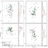 |
Fig. 5 Dust mass abundances obtained from fitting the SED of each region using a 4 Myr ISRF and Compiegne dust model. Only fits with a |
4.2. Morphology and dust properties
We show here that YVSG/YTOTAL is higher for filled and mixed regions by a factor of ~1.7. This trend allows us to understand the change in dust properties in different environments and to shed light on the dust evolution in the ISM. Jones et al. (1996) showed that dust grain-grain collisions, commonly referred to as shattering, lead to fragmentation of the entire grain, or part of it, into smaller distinct subgrains. Figure 13 c of Jones et al. (1996) shows that large grains (radii >400 Å) are disrupted by a single 100 km s-1 shock and that the grain mass is transferred to smaller grains. This mass transfer is seen in the resulting post-shock grain size distribution (Fig. 17 in that paper). Moreover, the adoption of a different initial grain size spectrum does not greatly affect the final grain size distribution, as shown in Jones et al. (1996). A re-evaluation of the dust processing effects in shocks has been performed by Bocchio et al. (2014). These authors used the new dust model from Jones et al. (2013), which assumes only two grain types (hydrogenated amorphous carbon and large amorphous silicate grains), and found that both carbonaceous and silicate grains undergo more destruction than in the previous studies, but the silicates are more resilient to shocks than the carbonaceous grains. Since we kept the ratio of the silicates and carbonaceous fixed in our models, we are unable to test this further.
Our sample of H ii regions classified as filled and mixed have central clusters rich in massive stars that produce strong stellar winds and create high-velocity (~50–90 km s-1, according to Relaño & Beckman 2005) expansive structures in their interiors. For these regions a higher fraction of YVSG/YTOTAL compared to more quiescent environments is therefore expected according to the Jones et al. (1996) dust evolution model. Shell and clear shell objects in our sample are in a more evolved and quiescent state. They have already swept up all the gas and dust in their close surroundings and show prominent shell structures not only in Hα, but also in the longer wavelengths 250 μm, 350 μm, and 500 μm of SPIRE (see Fig. 3 of Verley et al. 2010). We expect these regions to have much lower shock velocities because they are in a more evolutionary state, and therefore to present a lower relative fraction of VSGs. This agrees with the results presented in Stephens et al. (2014), who showed that for the most evolved H ii region in their sample, a superbubble named N70, YVSG/YTOTAL is lower than for the less evolved H ii regions in their sample. Another interpretation of the observed shell structures in the SPIRE bands could be the reformation of dust BGs through coagulation and accretion in dense clouds, as has also been suggested by Jones et al. (1996). Stepnik et al. (2003) proposed grain-grain coagulation as the main mechanism to explain the deficit of the IRAS I(60 μm)/I(100 μm) flux ratio in the Taurus molecular complex compared to the diffuse ISM. The same region was studied by Ysard et al. (2013) using DustEM, who found that the observed SED at different locations within the complex could be explained by changes in the optical properties of the grains. Paradis et al. (2009) found an increase in FIR emissivity in molecular clouds along the Galactic plane with significantly colder dust and interpreted it as coagulation of dust grains into fractal aggregates. Although reformation of BGs is not excluded as a mechanism to explain the shell structures observed in the SPIRE bands, detailed estimations of the dust temperature of the BGs and the density of the ISM in these regions are required to check the viability of this phenomenon (Köhler et al. 2012). For example, Köhler et al. (2015) found that coagulation and accretion produce significant changes in the dust properties that can explain the observed SED variations between diffuse and denser regions.
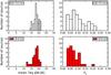 |
Fig. 6 Dust temperature (left) and F0 (right) distributions for filled and mixed together, and shell morphologies. The dust temperature is defined as the mean of the equilibrium temperature of all aSil grains with different sizes. |
4.3. Dust temperature
To study the temperature of the dust for each H ii region in our sample, we made use of the equilibrium temperature provided by DustEM. The code provides the equilibrium temperature of the LamC and aSil grains for each size. For each grain type, we estimated the dust temperature as the mean value of the equilibrium temperature of all aSil grains with different sizes as in Ysard et al. (2013). Other authors used the equilibrium temperature of the most populated dust grain (Flagey et al. 2011), we verified that the conclusions of this section do not change when this other definition of the dust temperature is used. We made use of the aSil grains because they are more abundant than LamC grains, and the relative fraction between them was kept constant in our fitting (see Sect. 3.2). In the left-hand panel of Fig. 6 we show the distribution of the dust temperature for each morphological classification. Only a slight trend is visible for the distribution of the shells and clear shells to extend to lower temperatures, while the distribution for the filled and mixed regions is narrower, with a peak at ~18 K. We find a mean dust temperature of 18.3 ± 0.3 K and 17.8 ± 0.4 K for filled and mixed together, and shell type objects, respectively, which shows that there is no significant difference in the dust temperature for each classification.
We also performed the same analysis using the classical definition of dust temperature from a modified blackbody (MBB) fitting. We used observational data in the 100–870 μm wavelength range, as the expected contribution of the stochastically heated grains in this wavelength range is negligible (for our set of H ii regions the best fits give a mean contribution of ~10% of the VSGs to the 100 μm band). We adopted the simple approach to keep β = 2 fixed and restricted the analysis to those fits with  (
( is defined as χ2/n, where n is the number of degrees of freedom, and χ2 = ∑ (Fobs−Fmod)2/σ2) and with a model 70 μm flux lower than observed. In total we worked with a set of 71 H ii regions: 7 filled, 35 mixed, and 29 shell and clear shell objects. We found a mean dust temperature of 17.9 ± 0.6 K, and 15.5 ± 0.6 K for filled and mixed, and shell type objects, respectively.
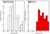 |
Fig. 7 250 μm emission relative to the TIR emission distribution for both filled and mixed together (left), and shell morphologies (right). The TIR emission is obtained using the prescription given by Boquien et al. (2011) including SPIRE and Herschel data from 24 to 250 μm. |
The equilibrium temperature for the BGs obtained with DustEM does not show any trend with morphology, while the dust temperature derived from the MBB shows differences that are slightly larger than 3σ. Based on these results, we cannot conclude that there is a statistically significant difference in the dust temperature distributions, but we find evidence from the MBB analysis that H ii regions of shell type might have the lowest temperatures. This trend can be understood from the different star-to-dust geometries in the H ii regions because within filled and mixed regions the dust and gas is probably mixed and closer to the stars that heat the dust than in the shells and clear shells regions. In the right panel of Fig. 6 we show the distribution of F0, a measure of the radiation field intensity (see Sect. 3.3), for both filled and mixed, and shell type regions, showing that shell objects are lacking the high values of F0 that are present in some filled and mixed types. We find mean values of F0 of 0.103 ± 0.008, and 0.076 ± 0.006 for filled and mixed, and shell type objects, respectively.
We cannot rule out that other mechanisms produce this slight difference in the dust temperature such as a higher fraction of BGs in the shell regions that would imply cooler grains than for the filled and mixed objects. We have shown that the relative fraction of VSGs is lower in the filled and mixed regions (see Fig. 5). It is also worthwhile to note that the emission at 250 μm relative to the TIR emission, an indicator of the dust temperature and/or the relative amount of BGs, presents higher values for shell regions than for filled and mixed objects (see Fig. 7): the mean value of the 250 μm/TIR ratio for shell regions is 0.73 ± 0.04, while for filled and mixed objects it is 0.53 ± 0.03.
The trends shown here are consistent with previous results given in the literature. Paper I presented evidence of a far-IR peak shifted towards longer wavelengths in the SED of H ii regions classified as shell and clear shell objects, which points to a colder dust in this type of objects. Verley et al. (2010) showed examples of filled and clear shell regions where the dust emission distribution observed in different bands of Spitzer and Herschel differs from band to band. Filled regions tend to show emission in all IR bands, while clear shell objects do not show any emission at 24 μm, and the emission in the SPIRE bands delineates the shell structure of the region. The authors suggested an evolutionary scenario where the dust is affected by the expansion of the gas within the region. The filled regions would be younger. The stellar winds would not have been able to create a cavity yet, therefore the dust and ionised gas are mixed within the region. They present emission at 24 μm inside the region, indicating that the dust is warm for these objects. The clear shell objects, however, would be more evolved. The expanding structure would have been created and the dust would have been swept up together with the ionised gas. The lack of emission at 24 μm and the presence of SPIRE emission at the shells shows that the dust is cooler for these objects.
4.4. Gas-to-dust mass ratio
Using the available HI and CO data, we are able to derive the gas mass within the aperture of each H ii region in the sample. The DustEM fits provide the dust mass for each region, and therefore we can obtain the gas-to-dust mass ratio in our sample. The molecular mass was obtained using the 12CO(J = 2–1) and HI intensity maps presented in Druard et al. (2014) and Gratier et al. (2010), respectively. The data were smoothed and registered to the SPIRE 250 μm spatial resolution and pixel size, and photometry was extracted following the procedure explained in Sect. 3.1. We used a CO-to-H2 conversion factor of  ), which is the one applied by Druard et al. (2014) and consistent with the metallicity of M 33. We then applied Eq. (3) from Druard et al. (2014), which assumes a constant ICO(2−1)/ICO(1−0), to derive the molecular hydrogen mass MH2 for each H ii region. The HI mass was obtained using a conversion factor for HI of 1.8 × 1018 cm-2/ (K km s-1), as in Gratier et al. (2010). In both cases we took the fraction of helium mass with a correction of 37% into account. The total gas mass is the sum of the neutral HI and the molecular H2 mass (Mtot = MHI + MH2).
In Fig. 8 we show the total gas surface density Σgas(MHI + MH2) versus the dust surface density Σdust for the H ii regions in our sample. As in the other sections in the paper, we use only those regions showing reliable fits ( ), and we also exclude five regions without CO emission within the defined apertures. In general, the distribution in Fig. 8 tends to flatten at high Σdust, as has been recently observed in the N11 star-forming complex of the LMC (Galametz et al. 2016). Analysing the distribution in more detail, we see that two regimes separated at a value of Σdust = 0.06 M⊙/ pc2 seem to coexist, as has been shown for the LMC and SMC in Roman-Duval et al. (2014). The distributions of the Σgas(MHI + MH2) and Σdust are different for values higher and lower than Σdust = 0.06 M⊙/ pc2 with a p-value from the KS test of lower than 1% in both cases. Σdust ~ 0.06 M⊙/ pc2 is a reference value to separate the diffuse atomic and molecular ISM at the metallicity of M 33. This value corresponds to a visual extinction of AV ~ 0.4 mag (see Roman-Duval et al. 2014), and Krumholz et al. (2009) showed that the H i−H2 transition occurs for AV = 0.2−0.4 mag at Z ~ 0.5 Z⊙ (see their Fig. 1). Regions with Σdust< 0.06 M⊙/ pc2 are in the H i diffuse regime, where a significant fraction of H2 molecular gas is dissociated, while regions with Σdust> 0.06 M⊙/ pc2 correspond to a molecular phase where the H2 is not dissociated. In our sample of regions, we obtain median values of MH2/MHI = 0.41 ± 0.06 and MH2/MHI = 0.88 ± 0.08 for the diffuse atomic and molecular regimes, confirming that Σdust = 0.06 M⊙/ pc2 indeed separates molecular and atomic dominated regions.
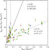 |
Fig. 8 Total gas surface density versus the dust surface density for the H ii regions in our sample with fits presenting |
We treated the two regimes separately and performed linear fits in each one (see Fig. 8). The derived slopes account for the gas-to-dust ratio in both regimes. The slope for the H i diffuse regime, 390 ± 68, is closer to the value of the gas-to-dust ratio expected from the metallicity of M 33, (gas-to-dust ~325, following the empirical broken power law given by Rémy-Ruyer et al. 2014) than the gas-to-dust ratio derived for the molecular regime, 67 ± 11. We note, however, that other gas-to-dust ratios derived for M 33 using a modified blackbody fitting range from 250 to 180, e.g. Kramer et al. (2010) and Hermelo et al. (2016). All of this shows the importance of using physically motivated dust models because the results might change significantly depending on the model. The slope obtained from the fit in the molecular regime gives a value thatisaboutfive times lower than the one derived in the H i diffuse regime, in agreement with the difference found between the slopes of the two regimes observed in the LMC by Roman-Duval et al. (2014).
These authors presented a detailed study of the possibilities causing the different slopes. One of the options is a different X(CO) factor for the diffuse atomic and molecular regimes. However, to bring the slopes of the two regimes into agreement with the gas-to-dust ratio expected from the metallicity in M 33, we would need a higher X(CO) factor in the molecular dense regime. Recent models from Shetty et al. (2011) show the opposite, the X(CO) factor would decrease in denser regions. Other physical explanations proposed by Roman-Duval et al. (2014) are the existence of grain coagulation and/or accretion of gas-phase metals onto dust grains. Grain coagulation would imply a constant dust mass fraction, as in this process it is the dust size distribution which is altered, keeping the total dust mass constant. Coagulation of VSGs into BGs can produce an enhancement in the dust opacity at long wavelengths (Köhler et al. 2012, 2015), and thus the emissivity of the BGs would be enhanced in the FIR part of the SED. The result would be an overestimation of the dust mass. In the grain accretion process, gas-phase metals will be incorporated into the dust mass and thus will produce an increase of the dust-to-gas ratio. To shed light onto the physical mechanisms that can cause the difference in the slopes for the two regimes, we plan to perform a detailed study of the dust-to-gas ratio variations in M 33 using DustEM models selecting an appropriate sample of spatial regions in this galaxy that is characteristic of the H i and molecular diffuse regimes (Relaño et al., in prep.).
5. Spatially resolved analysis: NGC 604 and NGC 595
The spatial resolution of Herschel data allows us to analyse the interior of the largest and most luminous H ii regions in M 33: NGC 604 and NGC 595. The Hα emission of NGC 604 reveals large cavities of ionised gas (see Fig. 2 in Relaño & Kennicutt 2009) produced by the stellar winds coming from the central star clusters. Stellar population studies in this region present evidence of Wolf Rayet (WR) stars (Hunter et al. 1996) and red supergiants (RSGs; Eldridge & Relaño 2011), showing two distinct formation episodes with ages 3.2 ± 1.0 Myr and 12.4 ± 2.1 Myr (Eldridge & Relaño 2011).
NGC 595 is the second most luminous H ii region in M 33. The Hα emission presents an open arc structure with a bright knot in the centre where the most massive stars are located (Relaño et al. 2010). The region also hosts numerous OB-type and RSG stars (Malumuth et al. 1996), as well as WR stars (Drissen et al. 2008). Malumuth et al. (1996) derived an age of 4.5 ± 1.0 Myr for the stellar population of NGC 595, which was later confirmed by Pellerin (2006). Pérez-Montero et al. (2011) performed a detailed modelling of NGC 595 using CLOUDY (Ferland et al. 1998) in a set of concentric elliptical annuli. These authors were able to fit the optical integral field spectroscopic observations from Relaño et al. (2010) and mid-infrared observations from Spitzer. The 8 μm/24 μm ratio was successfully fitted with a dust-to-gas ratio that increases radially from the centre to the outer parts of the region. The spatial distribution of the dust emission at 24 μm correlates with the emission at Hα for both H ii regions, showing that hot dust is mixed with the ionised gas in both objects (Relaño & Kennicutt 2009).
For the whole surface of NGC 604 and NGC 595 we performed a pixel-by-pixel SED modelling using DustEM and derived maps for each free parameter in the fit. We imposed a limit on the surface brightness at 250 μm to constrain the spatial emission of the H ii regions and to discard pixels with low surface brightness that have high uncertainties in their fluxes. We assumed a 4 Myr and 104 M⊙ star cluster ISRF that accounts for the age and stellar mass of the two regions.
5.1. Maps of the relative mass abundance of grains
In Figs. 9 and 10 we show the results of the SED fitting on a pixel-by-pixel basis. F0 correlates with FUV emission, which seems plausible because F0 is a measurement of the ISRF intensity coming from the stars within the region. The spatial distribution of the YVSG/YTOTAL map in both regions resembles the form of arcs and shells bordering the Hα emission, and the relative fraction of PAHs, YPAH/YTOTAL, tends to be higher around the region. Finally, the YBG/YTOTAL distribution in the central areas of both regions tends to show high values at the location of high emission in CO. All these maps show that the relative mass abundance of each grain type changes within the region depending on the local properties of the environment.
5.2. Signature of dust evolution within the regions
Evolution of the interstellar dust implies a redistribution of the dust mass in the different grain types through coagulation of small grains or fragmentation of large ones. Thus, a map of the relative mass fraction of VSG to BG would show the locations where these processes might take place. In the two maps in Fig. 11 the maxima in YVSG/YBG seem to be bordering the Hα emission. Jones et al. (1996) predicted that the fragmentation of BGs into VSGs occurs for shocks with velocities of at least of 50 km s-1. Therefore, we expect expanding structures with similar velocities at the location of YVSG/YBG enhancements. Yang et al. (1996) studied the kinematics of NGC 604 and found five shell structures within the region with expansion velocities of 40–125 km s-1 traced by the Hα emission line. The approximate locations of the centre of the shells are depicted in Fig. 11 with numbers. All of them are within the area where the maxima of YVSG/YBG are located. The kinematics of the ionised gas in the interior of NGC 595 was studied by Lagrois & Joncas (2009). These authors found two expanding shells located close to the position where the maximum of YVSG/YBG occurs and estimated a mean expansion velocity for the two shells of ~20 km s-1.
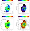 |
Fig. 9 F0 (top left), YVSG/YTOTAL (top right), YPAH/YTOTAL (bottom left), and YBG/YTOTAL (bottom right) distribution maps of NGC 604 obtained using DustEM with an ISRF representing a 4 Myr star cluster. The contours are FUV, Hα, Hα, and CO emission for the F0, YVSG/YTOTAL, YPAH/YTOTAL, and YBG/YTOTAL distribution maps, respectively. The spatial resolution of the contours are 4.4′′, 6.6′′, 3.0′′, and 20′′, respectively. |
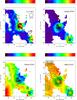 |
Fig. 10 F0 (top-left), YVSG/YTOTAL (top-right), YPAH/YTOTAL (bottom-left), and YBG/YTOTAL (bottom-right) distribution maps of NGC 595 obtained using DustEM with an ISRF representing a 4 Myr star cluster, as was done in previous sections. The contours are FUV, Hα, Hα, and CO emission for the F0, YVSG/YTOTAL, YPAH/YTOTAL, and YBG/YTOTAL distribution maps, respectively. The spatial resolution of the contours are 4.4′′, 6.6′′, 3.0′′, and 20′′, respectively. |
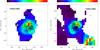 |
Fig. 11 YVSG/YBG distribution map for NGC 604 (left) and NGC 595 (right) obtained using DustEM code with a 4 Myr star cluster ISRF for NGC 604 and for NGC 595. The contours correspond to the continuum-subtracted Hα image at high resolution (6′′) and the numbers refer to the location of the expanding ionized gas shells observed by Yang et al. (1996) for NGC 604 and Lagrois & Joncas (2009) for NGC 595. Pixel size is 6′′. |
5.3. CO emission
In Fig. 12 we compare the YPAH/YTOTAL maps with CO(2–1) intensity distribution from Druard et al. (2014). The YPAH/YTOTAL distribution follows the CO(2–1) emission with the maximum in CO intensity corresponding to a minimum of YPAH/YTOTAL. The most intense CO(2–1) knot in NGC 604 is located close to source 1 of Martínez-Galarza et al. (2012). These authors observed NGC 604 with the Spitzer Infrared Spectrograph (IRS) and selected seven sources of interest based on their IRAC colours. In the left panel of Fig. 12 we show the location of sources 1 and 4, which exhibit the highest softness parameter η′, a tracer of the hardness of the ISRF, in the MIR (![Mathematical equation: \hbox{$\eta\prime =\rm \frac{I([Ne\,\textsc {ii}]12.8\,\mu m)/I([Ne\,\textsc {iii}]15.6\,\mu m)}{I([S\,\textsc {iii}]18.7\,\mu m)/I([S\,\textsc {iv}]10.5\,\mu m)}$}](/articles/aa/full_html/2016/11/aa28139-16/aa28139-16-eq85.png) , as it is defined in Pérez-Montero & Vílchez 2009). In addition, sources 1 and 4 also present the highest (6.2 μm + 7.7 μm + 8.6 μm)/11.3 μm ratio. The 11.3 μm PAH feature is associated with neutral PAHs, while 6.2 μm, 7.7 μm and 8.6 μm are associated with ionised PAHs. The location of sources 1 and 4, where a minimum in the YPAH/YTOTAL distribution is located, therefore shows the highest ionised/neutral PAH ratio and the hardest spectrum of all the sources analysed by Martínez-Galarza et al. (2012). The anti-correlation YPAH/YTOTAL-hardness of ISRF provides evidence that the PAHs appear to be destroyed in places where the ISRF is strong and hard, as has also been suggested in previous studies (Madden et al. 2006; Wu et al. 2006; Lebouteiller et al. 2007).
, as it is defined in Pérez-Montero & Vílchez 2009). In addition, sources 1 and 4 also present the highest (6.2 μm + 7.7 μm + 8.6 μm)/11.3 μm ratio. The 11.3 μm PAH feature is associated with neutral PAHs, while 6.2 μm, 7.7 μm and 8.6 μm are associated with ionised PAHs. The location of sources 1 and 4, where a minimum in the YPAH/YTOTAL distribution is located, therefore shows the highest ionised/neutral PAH ratio and the hardest spectrum of all the sources analysed by Martínez-Galarza et al. (2012). The anti-correlation YPAH/YTOTAL-hardness of ISRF provides evidence that the PAHs appear to be destroyed in places where the ISRF is strong and hard, as has also been suggested in previous studies (Madden et al. 2006; Wu et al. 2006; Lebouteiller et al. 2007).
The hardness of the ISRF at this particular location within NGC 604 might be produced by newly formed massive stars. Source 1 in the left panel of Fig. 12 is related to the maxima in CO(2–1) emission within the region and corresponds to the molecular cloud NMA-8, the most massive in NGC 604 (Miura et al. 2010). Miura et al. (2010) also studied the HCN emission distribution, a tracer of dense regions in molecular clouds where star formation can occur. They found that a HCN cloud lies at the location of NMA-8, whose maximum is shifted from the maximum of NMA-8 towards the centre of the region. They concluded that NMA-8 is a dense molecular cloud that could be in a stage of ongoing massive star formation. At the maxima of NMA-8, Relaño & Kennicutt (2009) found a difference between the extinction derived from the Balmer emission and the extinction derived from the Hα-24 μm ratio. The difference (also reported by Maíz-Apellániz et al. 2004, comparing Balmer and radio extinctions) might be produced if the surface of the molecular cloud has a shell morphology that would produce a lower value of the Balmer extinction. Relaño & Kennicutt (2009) suggested that there could be embedded star formation at this location based on a colour magnitude diagram analysis of NGC 604.
In the bottom left panels of Figs. 9 and 10 we compare the CO(2–1) emission distribution with the distribution of YBG/YTOTAL for NGC 604 and NGC 595, respectively. The maximum of the CO intensity is correlated with local maxima of the YBG/YTOTAL in both regions. This shows that CO is more closely related to the total dust mass, traced by the mass fraction of BGs, than to the PAH abundance in these regions. For NGC 595, the distribution of YBG follows the same radial pattern as the dust-to-gas ratio obtained from the modelling of the region performed by Pérez-Montero et al. (2011). These authors found that to fit the radial trend of the 8 μm/24 μm ratio, the dust-to-gas ratio assumed in the model needed to increase from the centre to the outer parts of the regions. Whether a change in the dust-to-gas ratio is related to a change in the YBG/YTOTAL due to grain coagulation or reformation requires a detailed study, which is beyond the scope of this paper.
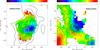 |
Fig. 12 YPAH/YTOTAL distribution map for NGC 604 (left) and NGC 595 (right) as shown in Figs. 9 and 10 overlaid with CO(2–1) intensity contours from Druard et al. (2014). The spatial resolution for both maps is 20′′ and the pixel size is 6′′. |
6. Summary and conclusions
We analysed the SEDs of a sample of 119 H ii regions classified in M 33 as filled, mixed, and shell and clear shell regions. The performed classification was based on the Hα emission distribution of each object and represents different star-gas-dust spatial configurations within the regions. We updated and completed the observed SEDs of Paper I with new data from Herschel at 70 μm, WISE at 3.4 μm, 4.6 μm, 12 μm, and 22 μm, and LABOCA at 870 μm. We studied the physical properties of the dust in different environments by fitting the observed SED of each region with the dust model of Compiègne et al. (2011) and analysing the results in terms of the region morphology. We analysed the relative mass for each grain type for the best SED fit of each object in our sample with two different ISRFs: a Mathis ISRF corresponding to the default solar neighbourhood (Mathis et al. 1983), and a more realistic one of a young 4 Myr cluster with a fixed stellar mass of 104 M⊙. We also used the approximation of a MBB to describe the emission of the dust and to fit the IR part of the observed SED. We summarise our main results below.
-
All the mass ratios obtained with the modelling were independent of the shape of the ISRF except for PAHs. YPAH/YTOTAL is a factor of 2–10 higher assuming a Mathis ISRF, which shows the difficulty of constraining the relative abundance of PAHs with the models used here. BGs represent the highest fraction of dust mass in the regions (~90%), while the relative mass of the PAHs is in general low (1–10%).
-
YVSG/YTOTAL is higher for filled and mixed regions by a factor of ~1.7 than for regions classified as shells and clear shells. The difference was the same when we applied the classic Desert dust model. We interpreted this result within the dust evolution framework proposed by Jones et al. (1996) where large grains can be disrupted by strong shocks. The regions classified as filled and mixed have high-velocity ~50–90 km s-1 expansive structures that can produce an enhancement of the relative fraction of VSGs, while the shells and clear shells present a more quiescent environment where the BGs can survive or reform.
-
We derived an estimate of the dust temperature using the equilibrium temperature of the aSil grains provided by DustEM. We found no difference in the temperature for filled and mixed regions and shell objects. However, a MBB analysis gives temperatures slightly higher than 3σ for the filled and mixed regions (T = 17.9 ± 0.6 K) than for the shell objects (T = 15.5 ± 0.6 K). This might be due to differences in the total dust opacity of the different types of H ii regions and/or to a different spatial distribution of dust and stars within the types of the regions.
-
We derived the gas-to-dust ratio for the H ii regions in our sample from the slope of the dust-gas surface density relation. We found two different slopes in the relation: regions with Σdust< 0.06 M⊙/ pc2, corresponding to the H i diffuse regime, present a gas-to-dust ratio of 390 ± 68 compatible with the expected value if we assume that the gas-to-dust ratio scales linearly with metallicity. Regions with Σdust ≥ 0.06 M⊙/ pc2, corresponding to a H2 molecular phase, present a flatter dust-gas surface density distribution, with a corresponding gas-to-dust ratio of 67 ± 11. These variations might imply that grain coagulation and/or gas-phase metal incorporation into the dust mass occurs in the interior of the H ii regions in M 33.
-
In a spatially resolved analysis, we performed a pixel-by-pixel SED fitting of the whole surface of the two most luminous H ii regions in M33: NGC 604 and NGC 595. We derived maps of the relative mass fraction of VSG to BG (YVSG/YBG) for NGC 604 and NGC 595. We found local maxima of YVSG/YBG correlated to expansive ionised gas structures with velocities ≳50 km s-1 within the regions. This agrees with the results of Jones et al. (1996), who predicted the fragmentation of BGs into VSGs as a result of shocks with velocities of at least 50 km s-1.
-
YPAH/YTOTAL distribution for NGC 604 and NGC 595 follows the CO(2–1) emission, with the maximum in CO intensity corresponding to a minimum of YPAH/YTOTAL. A deeper analysis using IRS data for NGC 604 showed that the minimum of YPAH/YTOTAL in this region corresponds to a highly ionised or neutral PAH ratio and the location of a hard ISRF. This is evidence that the PAHs are destroyed in places where the ISRF is strong and hard.
The dust emission in the IR has been shown to be a tracer of the star formation in a galaxy, and correlations, albeit with dispersions, have been presented in the literature between the IR bands and other, more direct, star formation rate tracers, such as the Hα emission coming from the ionised gas heated by recently formed stars. The emission in the 24 μm band has been particularly successful in tracing the star formation in H ii regions, as it corresponds to the warm dust mixed with the hot ionised gas at these locations (see e.g. Calzetti et al. 2005). However, we showed here that the relative fraction of VSGs, which are the main contributors to the 24 μm band emission, is not constant but changes (a factor of 1.7) depending on the morphology (and the evolutionary state) of the region. This effect introduces an uncertainty in the correlation between the 24 μm and Hα emission, which is expected to contribute to the dispersion in the observed empirical correlation. Understanding the physical properties of the dust, in particular the variation of the VSGs in different H ii regions, will help us to better understand the uncertainties in the empirical correlations between SFR tracers.
This publication is based on data acquired with the Atacama Pathfinder Experiment (APEX) under programme IDs 085.F-0045, 086.F-9301, and 089.C-0935. APEX is a collaboration between the Max-Planck-Institut für Radioastronomie, the European Southern Observatory, and the Onsala Space Observatory.
Acknowledgments
We would like to thank the referee for the useful comments that helped to improve the first version of this paper. Part of this research has been supported by the PERG08-GA-2010-276813 from the EC. This work was partially supported by the Junta de Andalucía Grant FQM108 and Spanish MEC Grants, AYA-2011-24728 and AYA-2014-53506-P. EPM thanks Spanish MINECO grant AYA-2013-47742-C4-1-P of the Spanish Plan for Astronomy and Astrophysics. This work was in part supported through NSF ATI grant 1106284. This research made use of Montage, funded by the National Aeronautics and Space Administration’s Earth Science Technology Office, Computational Technnologies Project, under Cooperative Agreement Number NCC5-626 between NASA and the California Institute of Technology. The code is maintained by the NASA/IPAC Infrared Science Archive. M.R. would like to thank L. Vestreate and D. Paradis for their help with DustEM code. M.A. acknowledges funding by the German Research Foundation (DFG) in the framework of the priority programme 1573, “The Physics of the Interstellar Medium”, through grant number AL 1467/2-1. This research made use of APLpy, an open-source plotting package for Python hosted at http://aplpy.github.com of TOPCAT & STIL: Starlink Table/VOTable Processing Software (Taylor 2005) of Matplotlib, a suite of open-source python modules that provide a framework for creating scientific plots.
References
- Aniano, G., Draine, B. T., Calzetti, D., et al. 2012, ApJ, 756, 138 [NASA ADS] [CrossRef] [Google Scholar]
- Bernard, J.-P., Reach, W. T., Paradis, D., et al. 2008, AJ, 136, 919 [NASA ADS] [CrossRef] [Google Scholar]
- Bocchio, M., Jones, A. P., & Slavin, J. D. 2014, A&A, 570, A32 [NASA ADS] [CrossRef] [EDP Sciences] [Google Scholar]
- Boquien, M., Calzetti, D., Combes, F., et al. 2011, AJ, 142, 111 [NASA ADS] [CrossRef] [Google Scholar]
- Boquien, M., Calzetti, D., Aalto, S., et al. 2015, A&A, 578, A8 [NASA ADS] [CrossRef] [EDP Sciences] [Google Scholar]
- Bresolin, F. 2011, ApJ, 730, 129 [NASA ADS] [CrossRef] [Google Scholar]
- Calzetti, D., Kennicutt, R. C., Bianchi, L., et al. 2005, ApJ, 633, 871 [NASA ADS] [CrossRef] [Google Scholar]
- Calzetti, D., Kennicutt, R. C., Engelbracht, C. W., et al. 2007, ApJ, 666, 870 [NASA ADS] [CrossRef] [Google Scholar]
- Cardelli, J. A., Clayton, G. C., & Mathis, J. S. 1989, ApJ, 345, 245 [NASA ADS] [CrossRef] [Google Scholar]
- Churchwell, E., Babler, B. L., Meade, M. R., et al. 2009, PASP, 121, 213 [NASA ADS] [CrossRef] [Google Scholar]
- Compiègne, M., Abergel, A., Verstraete, L., & Habart, E. 2008, A&A, 491, 797 [NASA ADS] [CrossRef] [EDP Sciences] [Google Scholar]
- Compiègne, M., Verstraete, L., Jones, A., et al. 2011, A&A, 525, A103 [NASA ADS] [CrossRef] [EDP Sciences] [Google Scholar]
- Desert, F.-X., Boulanger, F., & Puget, J. L. 1990, A&A, 237, 215 [NASA ADS] [Google Scholar]
- Draine, B. T., & Li, A. 2007, ApJ, 657, 810 [NASA ADS] [CrossRef] [Google Scholar]
- Drissen, L., Crowther, P. A., Úbeda, L., et al. 2008, MNRAS, 389, 1033 [NASA ADS] [CrossRef] [Google Scholar]
- Druard, C., Braine, J., Schuster, K. F., et al. 2014, A&A, 567, A118 [NASA ADS] [CrossRef] [EDP Sciences] [Google Scholar]
- Eldridge, J. J., & Relaño, M. 2011, MNRAS, 411, 235 [NASA ADS] [CrossRef] [Google Scholar]
- Ferland, G. J., Korista, K. T., Verner, D. A., et al. 1998, PASP, 110, 761 [Google Scholar]
- Flagey, N., Boulanger, F., Verstraete, L., et al. 2006, A&A, 453, 969 [NASA ADS] [CrossRef] [EDP Sciences] [Google Scholar]
- Flagey, N., Boulanger, F., Noriega-Crespo, A., et al. 2011, A&A, 531, A51 [NASA ADS] [CrossRef] [EDP Sciences] [Google Scholar]
- Freedman, W. L., Wilson, C. D., & Madore, B. F. 1991, ApJ, 372, 455 [NASA ADS] [CrossRef] [Google Scholar]
- Galametz, M., Hony, S., Albrecht, M., et al. 2016, MNRAS, 456, 1767 [NASA ADS] [CrossRef] [Google Scholar]
- Galliano, F., Dwek, E., & Chanial, P. 2008, ApJ, 672, 214 [NASA ADS] [CrossRef] [Google Scholar]
- Gratier, P., Braine, J., Rodriguez-Fernandez, N. J., et al. 2010, A&A, 522, A3 [NASA ADS] [CrossRef] [EDP Sciences] [Google Scholar]
- Hermelo, I., Relaño, M., Lisenfeld, U., et al. 2016, A&A, 590, A56 [NASA ADS] [CrossRef] [EDP Sciences] [Google Scholar]
- Hunter, D. A., Baum, W. A., O’Neil, E. J., et al. 1996, ApJ, 456, 174 [NASA ADS] [CrossRef] [Google Scholar]
- Jarrett, T. H., Cohen, M., Masci, F., et al. 2011, ApJ, 735, 112 [NASA ADS] [CrossRef] [Google Scholar]
- Jarrett, T. H., Masci, F., Tsai, C. W., et al. 2013, AJ, 145, 6 [NASA ADS] [CrossRef] [EDP Sciences] [Google Scholar]
- Jones, A. P. 2004, in Astrophysics of Dust, eds. A. N. Witt, G. C. Clayton, & B. T. Draine, ASP Conf. Ser., 309, 347 [Google Scholar]
- Jones, A. P., Tielens, A. G. G. M., & Hollenbach, D. J. 1996, ApJ, 469, 740 [NASA ADS] [CrossRef] [Google Scholar]
- Jones, A. P., Fanciullo, L., Köhler, M., et al. 2013, A&A, 558, A62 [NASA ADS] [CrossRef] [EDP Sciences] [Google Scholar]
- Köhler, M., Stepnik, B., Jones, A. P., et al. 2012, A&A, 548, A61 [NASA ADS] [CrossRef] [EDP Sciences] [Google Scholar]
- Köhler, M., Ysard, N., & Jones, A. P. 2015, A&A, 579, A15 [NASA ADS] [CrossRef] [EDP Sciences] [Google Scholar]
- Kramer, C., Buchbender, C., Xilouris, E. M., et al. 2010, A&A, 518, L67 [NASA ADS] [CrossRef] [EDP Sciences] [Google Scholar]
- Kroupa, P. 2001, MNRAS, 322, 231 [NASA ADS] [CrossRef] [Google Scholar]
- Krumholz, M. R., McKee, C. F., & Tumlinson, J. 2009, ApJ, 693, 216 [NASA ADS] [CrossRef] [Google Scholar]
- Lagrois, D., & Joncas, G. 2009, ApJ, 700, 1847 [NASA ADS] [CrossRef] [Google Scholar]
- Lebouteiller, V., Brandl, B., Bernard-Salas, J., Devost, D., & Houck, J. R. 2007, ApJ, 665, 390 [NASA ADS] [CrossRef] [Google Scholar]
- Leitherer, C., Schaerer, D., Goldader, J. D., et al. 1999, ApJS, 123, 3 [NASA ADS] [CrossRef] [Google Scholar]
- Lu, N., Helou, G., Werner, M. W., et al. 2003, ApJ, 588, 199 [NASA ADS] [CrossRef] [Google Scholar]
- Madden, S. C., Galliano, F., Jones, A. P., & Sauvage, M. 2006, A&A, 446, 877 [NASA ADS] [CrossRef] [EDP Sciences] [Google Scholar]
- Maíz-Apellániz, J., Pérez, E., & Mas-Hesse, J. M. 2004, AJ, 128, 1196 [NASA ADS] [CrossRef] [Google Scholar]
- Malumuth, E. M., Waller, W. H., & Parker, J. W. 1996, AJ, 111, 1128 [NASA ADS] [CrossRef] [Google Scholar]
- Markwardt, C. B. 2009, in Astronomical Data Analysis Software and Systems XVIII, eds. D. A. Bohlender, D. Durand, & P. Dowler, ASP Conf. Ser., 411, 251 [Google Scholar]
- Martínez-Galarza, J. R., Hunter, D., Groves, B., & Brandl, B. 2012, ApJ, 761, 3 [NASA ADS] [CrossRef] [Google Scholar]
- Mathis, J. S., Mezger, P. G., & Panagia, N. 1983, A&A, 128, 212 [NASA ADS] [Google Scholar]
- Miura, R., Okumura, S. K., Tosaki, T., et al. 2010, ApJ, 724, 1120 [NASA ADS] [CrossRef] [Google Scholar]
- Ott, S. 2010, in Astronomical Data Analysis Software and Systems XIX, eds. Y. Mizumoto, K.-I. Morita, & M. Ohishi, ASP Conf. Ser., 434, 139 [Google Scholar]
- Ott, S. 2011, in Astronomical Data Analysis Software and Systems XX, eds. I. N. Evans, A. Accomazzi, D. J. Mink, & A. H. Rots, ASP Conf. Ser., 442, 347 [Google Scholar]
- Paradis, D., Bernard, J.-P., & Mény, C. 2009, A&A, 506, 745 [NASA ADS] [CrossRef] [EDP Sciences] [Google Scholar]
- Paradis, D., Paladini, R., Noriega-Crespo, A., et al. 2011, ApJ, 735, 6 [NASA ADS] [CrossRef] [Google Scholar]
- Pellerin, A. 2006, AJ, 131, 849 [NASA ADS] [CrossRef] [Google Scholar]
- Pérez-Montero, E., & Vílchez, J. M. 2009, MNRAS, 400, 1721 [NASA ADS] [CrossRef] [Google Scholar]
- Pérez-Montero, E., Relaño, M., Vílchez, J. M., & Monreal-Ibero, A. 2011, MNRAS, 412, 675 [NASA ADS] [CrossRef] [Google Scholar]
- Relaño, M., & Beckman, J. E. 2005, A&A, 430, 911 [NASA ADS] [CrossRef] [EDP Sciences] [Google Scholar]
- Relaño, M., & Kennicutt, R. C. 2009, ApJ, 699, 1125 [NASA ADS] [CrossRef] [Google Scholar]
- Relaño, M., Monreal-Ibero, A., Vílchez, J. M., & Kennicutt, R. C. 2010, MNRAS, 402, 1635 [NASA ADS] [CrossRef] [Google Scholar]
- Relaño, M., Verley, S., Pérez, I., et al. 2013, A&A, 552, A140 [NASA ADS] [CrossRef] [EDP Sciences] [Google Scholar]
- Rémy-Ruyer, A., Madden, S. C., Galliano, F., et al. 2014, A&A, 563, A31 [NASA ADS] [CrossRef] [EDP Sciences] [Google Scholar]
- Roman-Duval, J., Gordon, K. D., Meixner, M., et al. 2014, ApJ, 797, 86 [NASA ADS] [CrossRef] [Google Scholar]
- Roussel, H. 2013, PASP, 125, 1126 [Google Scholar]
- Sellgren, K., Werner, M. W., & Dinerstein, H. L. 1983, ApJ, 271, L13 [CrossRef] [Google Scholar]
- Shetty, R., Glover, S. C., Dullemond, C. P., & Klessen, R. S. 2011, MNRAS, 412, 1686 [NASA ADS] [CrossRef] [MathSciNet] [Google Scholar]
- Siringo, G., Kreysa, E., Kovács, A., et al. 2009, A&A, 497, 945 [NASA ADS] [CrossRef] [EDP Sciences] [Google Scholar]
- Staguhn, J. G., Benford, D. J., Allen, C. A., et al. 2006, SPIE Conf. Ser., 6275, 1 [Google Scholar]
- Stephens, I. W., Evans, J. M., Xue, R., et al. 2014, ApJ, 784, 147 [NASA ADS] [CrossRef] [Google Scholar]
- Stepnik, B., Abergel, A., Bernard, J.-P., et al. 2003, A&A, 398, 551 [NASA ADS] [CrossRef] [EDP Sciences] [Google Scholar]
- Tabatabaei, F. S., Beck, R., Krügel, E., et al. 2007, A&A, 475, 133 [NASA ADS] [CrossRef] [EDP Sciences] [Google Scholar]
- Taylor, M. B. 2005, in Astronomical Data Analysis Software and Systems XIV, eds. P. Shopbell, M. Britton, & R. Ebert, ASP Conf. Ser., 347, 29 [Google Scholar]
- van den Bergh, S. 2000, The galaxies of the Local Group (Cambridge University Press), 35 [Google Scholar]
- Verley, S., Relaño, M., Kramer, C., et al. 2010, A&A, 518, L68 [NASA ADS] [CrossRef] [EDP Sciences] [Google Scholar]
- Weiß, A., Kovács, A., Coppin, K., et al. 2009, ApJ, 707, 1201 [NASA ADS] [CrossRef] [Google Scholar]
- Whitmore, B. C., Chandar, R., Kim, H., et al. 2011, ApJ, 729, 78 [NASA ADS] [CrossRef] [Google Scholar]
- Wright, E. L., Eisenhardt, P. R. M., Mainzer, A. K., et al. 2010, AJ, 140, 1868 [NASA ADS] [CrossRef] [Google Scholar]
- Wu, Y., Charmandaris, V., Hao, L., et al. 2006, ApJ, 639, 157 [NASA ADS] [CrossRef] [Google Scholar]
- Xilouris, E. M., Tabatabaei, F. S., Boquien, M., et al. 2012, A&A, 543, A74 [NASA ADS] [CrossRef] [EDP Sciences] [Google Scholar]
- Yang, H., Chu, Y.-H., Skillman, E. D., & Terlevich, R. 1996, AJ, 112, 146 [NASA ADS] [CrossRef] [Google Scholar]
- Ysard, N., Abergel, A., Ristorcelli, I., et al. 2013, A&A, 559, A133 [NASA ADS] [CrossRef] [EDP Sciences] [Google Scholar]
Appendix A: Fluxes
Appendix B: Comparison of fluxes
In Fig. B.1 we show the comparison of the PACS 100 μm and 160 μm obtained here with the ones published in Paper I. The low luminosity regions tend to show higher fluxes than in previous images, which shows that the new images recover the missed flux in the previous ones. The comparison of PACS and MIPS 70 μm fluxes is shown in the left panels of Fig. B.1. In general PACS 70 μm fluxes are higher than MIPS 70 μm ones for bright regions. This trend is the same as it was found in Aniano et al. (2012) for NGC 628 and NGC 6946.
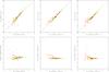 |
Fig. B.1 Left column: comparison of the MIPS and PACS 70 μm fluxes. Middle and right columns: comparison of the PACS 100 μm and 160 μm fluxes presented in this paper and those published in Paper I. |
Appendix C: SED fitting for Desert dust model
We show here the results of the SED fitting using the classical dust model from Desert et al. (1990). This model does not distinguish between neutral and ionised PAHs and therefore it is not able to fit properly the 6–9 μm wavelength range corresponding to ionised PAHs. All the SEDs in Fig. C.1 show high residuals in this wavelength range. However, as we can see from Fig. C.2, Desert dust model also predicts a higher YVSG for filled and mixed than for shells and clear shells, showing that the destruction of BGs into VSGs by strong shocks is mainly regulated by the size of the grains.
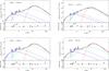 |
Fig. C.1 SED fittings for the 4 regions shown in Fig. 4 but fitted with a 4 Myr star cluster ISRF and Desert dust model. Light blue points: observed data with the errors, red squares: modelled broad-band fluxes, dashed-dot blue line: PAH emission, dashed-dot green line: VSG emission, dashed-dot red line: BG emission and dashed purple line: NIR continuum. The SED is well fitted at most bands except in the 6–9 μm wavelength range where the Desert dust model under-predicts the PAH emission. |
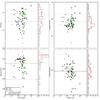 |
Fig. C.2 Dust mass abundances obtained fitting the SED of each region using 4 Myr ISRF and Desert dust model. Only fits with a |
Appendix D: Robustness of the best fit
The SED fitting is obtained based on the Levenberg-Marquardt minimisation method. We have explored the robustness of the fit using the best fit SED given by the minimisation method and creating a new fakeSED which is then fitted with the same initial parameters. We generate the new fluxes of the fake SED in each band choosing a random flux value from a Gaussian distribution having the best fit flux as a mean value and the observational uncertainty as σ. The best fit parameters of the new fit is then compared with those obtained initially. In Fig. D.1 we show the comparison for the parameters in the fit for each H ii region. The relative abundance of the grains derived from the fit are quite robust, however the differences in the ISRF scale seem to increase for higher values of F0.
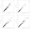 |
Fig. D.1 Robustness of the best fit for the F0 (top-left), YVSG (top-right), YPAH (bottom-left), and YBG (bottom-right). We use the best fit SED given by the minimisation method (YBestFit) and create a new SED choosing a random flux value in each band from a Gaussian distribution having the best fit flux as a mean value and the observational uncertainty as σ. The best fit parameters of the new fit (YNew) are then compared with those obtained initially from the minimisation method. |
All Tables
Statistics of YVSG/YTOTAL, YPAH/YTOTAL, and YBG/YTOTAL for each morphological type of the H ii regions in our sample.
All Figures
|
Fig. 1 2 mm image of NGC 604 observed with the GISMO continuum camera. The final spatial resolution of the image is 21.0′′ to match the other data. |
| In the text | |
|
Fig. 2 Comparison of Mathis et al. (1983) ISRF (dashed line) and an ISRF of a 4 Myr star cluster (continuous line; see text for details). Both ISRFs have been scaled to the same maximum intensity for a better comparison. The ISRF of a 4 Myr star cluster has a significant contribution in the UV part of the spectrum. |
| In the text | |
|
Fig. 3 Comparison of the DustEM output parameters for the H ii regions in our sample using a 4 Myr star cluster ISRF and a Mathis ISRF. Top left: scale factor of the ISRF intensity, top right: YVSG, bottom left: YBG, and bottom right: YPAH. The continuous line corresponds to the linear fit to the data and the dashed line is the one-to-one relation. The colour code corresponds to the morphology of the region classified in Paper I: blue circles are filled regions, green squares mixed ones, and red triangles shells or clear shells. |
| In the text | |
|
Fig. 4 Example of SED models for four regions of the sample catalogued as filled (top left), mixed (top right), shell (bottom left), and clear shell (bottom right). These regions correspond to regions 5, 98, 45, and 78 in Table B.1 in Paper I, respectively. Region 98 is the most luminous H ii region in M 33, NGC 604. The best-fit SED (continuous black line) is obtained assuming a 4 Myr star cluster ISRF and Compiegne dust model. Light blue points: observed data with the errors, red squares: modelled broad-band fluxes, dashed-dot blue line: total (ionised and neutral) PAH emission, dashed-dot green line: VSG (SamC) grain emission, dashed-dot red line: BG (LamC and aSil grains) emission, and dashed purple line: NIR continuum. |
| In the text | |
|
Fig. 5 Dust mass abundances obtained from fitting the SED of each region using a 4 Myr ISRF and Compiegne dust model. Only fits with a |
| In the text | |
|
Fig. 6 Dust temperature (left) and F0 (right) distributions for filled and mixed together, and shell morphologies. The dust temperature is defined as the mean of the equilibrium temperature of all aSil grains with different sizes. |
| In the text | |
|
Fig. 7 250 μm emission relative to the TIR emission distribution for both filled and mixed together (left), and shell morphologies (right). The TIR emission is obtained using the prescription given by Boquien et al. (2011) including SPIRE and Herschel data from 24 to 250 μm. |
| In the text | |
|
Fig. 8 Total gas surface density versus the dust surface density for the H ii regions in our sample with fits presenting |
| In the text | |
|
Fig. 9 F0 (top left), YVSG/YTOTAL (top right), YPAH/YTOTAL (bottom left), and YBG/YTOTAL (bottom right) distribution maps of NGC 604 obtained using DustEM with an ISRF representing a 4 Myr star cluster. The contours are FUV, Hα, Hα, and CO emission for the F0, YVSG/YTOTAL, YPAH/YTOTAL, and YBG/YTOTAL distribution maps, respectively. The spatial resolution of the contours are 4.4′′, 6.6′′, 3.0′′, and 20′′, respectively. |
| In the text | |
|
Fig. 10 F0 (top-left), YVSG/YTOTAL (top-right), YPAH/YTOTAL (bottom-left), and YBG/YTOTAL (bottom-right) distribution maps of NGC 595 obtained using DustEM with an ISRF representing a 4 Myr star cluster, as was done in previous sections. The contours are FUV, Hα, Hα, and CO emission for the F0, YVSG/YTOTAL, YPAH/YTOTAL, and YBG/YTOTAL distribution maps, respectively. The spatial resolution of the contours are 4.4′′, 6.6′′, 3.0′′, and 20′′, respectively. |
| In the text | |
|
Fig. 11 YVSG/YBG distribution map for NGC 604 (left) and NGC 595 (right) obtained using DustEM code with a 4 Myr star cluster ISRF for NGC 604 and for NGC 595. The contours correspond to the continuum-subtracted Hα image at high resolution (6′′) and the numbers refer to the location of the expanding ionized gas shells observed by Yang et al. (1996) for NGC 604 and Lagrois & Joncas (2009) for NGC 595. Pixel size is 6′′. |
| In the text | |
|
Fig. 12 YPAH/YTOTAL distribution map for NGC 604 (left) and NGC 595 (right) as shown in Figs. 9 and 10 overlaid with CO(2–1) intensity contours from Druard et al. (2014). The spatial resolution for both maps is 20′′ and the pixel size is 6′′. |
| In the text | |
|
Fig. B.1 Left column: comparison of the MIPS and PACS 70 μm fluxes. Middle and right columns: comparison of the PACS 100 μm and 160 μm fluxes presented in this paper and those published in Paper I. |
| In the text | |
|
Fig. C.1 SED fittings for the 4 regions shown in Fig. 4 but fitted with a 4 Myr star cluster ISRF and Desert dust model. Light blue points: observed data with the errors, red squares: modelled broad-band fluxes, dashed-dot blue line: PAH emission, dashed-dot green line: VSG emission, dashed-dot red line: BG emission and dashed purple line: NIR continuum. The SED is well fitted at most bands except in the 6–9 μm wavelength range where the Desert dust model under-predicts the PAH emission. |
| In the text | |
|
Fig. C.2 Dust mass abundances obtained fitting the SED of each region using 4 Myr ISRF and Desert dust model. Only fits with a |
| In the text | |
|
Fig. D.1 Robustness of the best fit for the F0 (top-left), YVSG (top-right), YPAH (bottom-left), and YBG (bottom-right). We use the best fit SED given by the minimisation method (YBestFit) and create a new SED choosing a random flux value in each band from a Gaussian distribution having the best fit flux as a mean value and the observational uncertainty as σ. The best fit parameters of the new fit (YNew) are then compared with those obtained initially from the minimisation method. |
| In the text | |
Current usage metrics show cumulative count of Article Views (full-text article views including HTML views, PDF and ePub downloads, according to the available data) and Abstracts Views on Vision4Press platform.
Data correspond to usage on the plateform after 2015. The current usage metrics is available 48-96 hours after online publication and is updated daily on week days.
Initial download of the metrics may take a while.