| Issue |
A&A
Volume 594, October 2016
|
|
|---|---|---|
| Article Number | A55 | |
| Number of page(s) | 47 | |
| Section | Stellar structure and evolution | |
| DOI | https://doi.org/10.1051/0004-6361/201628860 | |
| Published online | 13 October 2016 | |
ξTauri: a unique laboratory to study the dynamic interaction in a compact hierarchical quadruple system ⋆,⋆⋆
1 Astronomical Institute of the Charles University, Faculty of Mathematics and Physics, V Holešovičkách 2, 180 00 Praha 8, Troja, Czech Republic
2 Laboratoire Lagrange, OCA/UNS/CNRS UMR 7293, BP 4229, 06304 Nice Cedex, France
3 European Southern Observatory, Karl–Schwarzschild–Str. 2, 85748 Garching bei München, Germany
4 Department of Mathematics, Physics & Geology, Cape Breton University, 1250 Grand Lake Road, Sydney, NS B1P 6L2, Canada
5 Department of Physics & Astronomy, University of British Columbia, 6224 Agricultural Road, Vancouver, BC V6T 1Z1, Canada
6 Department of Astronomy and Astrophysics, University of Toronto, 50 St. George Street, Toronto, Ontario, M5S 3H4, Canada
7 Hvar Observatory, Faculty of Geodesy, Zagreb University, Kačićeva 26, 10000 Zagreb, Croatia
8 Astronomisches Institut, Ruhr-Universität Bochum, Universitätsstraße 150, 44780 Bochum, Germany
9 Instituto de Astronomía, Universidad Católica del Norte, Avenida Angamos 0610, Casilla 1280 Antofagasta, Chile
10 Department of Astronomy and Astrophysics, Villanova University, Villanova, PA 19085, USA
11 CHARA Array, Mount Wilson Observatory, Mount Wilson, CA 91023, USA
12 Department of Astronomy and Physics, Saint Mary’s University, Halifax, N.S., B3H 3C3, Canada
13 Astronomical Institute, Academy of Sciences of the Czech Republic, 251 65 Ondřejov, Czech Republic
14 Institute of Astronomy, University Vienna, Türkenschanzstrasse 17, 1180 Vienna, Austria
15 Department de Physique, Université de Montréal, C.P. 6128, Succursale Centre-Ville, Montréal, QC H3C 3J7, Canada
16 Observatório do Instituto Geográfico do Exército, R. Venezuela 29 3 Esq., 1500-618, Lisbon, Portugal
17 NASA Ames Research Center, Moffett Field, CA 94035; SETI Institute, Mountain View, CA 94043, USA
18 Université de Lyon, Université Lyon 1, École Normale Supérieure de Lyon, CNRS, Centre de Recherche Astrophysique de Lyon UMR 5574, 69230 Saint-Genis-Laval, France
19 US Naval Observatory, Flagstaff Station, 10391 West Naval Observatory Road, Flagstaff, AZ 86005-8521, USA
Received: 5 May 2016
Accepted: 27 May 2016
Context. Compact hierarchical systems are important because the effects caused by the dynamical interaction among its members occur ona human timescale. These interactions play a role in the formation of close binaries through Kozai cycles with tides. One such system is ξ Tauri: it has three hierarchical orbits: 7.14 d (eclipsing components Aa, Ab), 145 d (components Aa+Ab, B), and 51 yr (components Aa+Ab+B, C).
Aims. We aim to obtain physical properties of the system and to study the dynamical interaction between its components.
Methods. Our analysis is based on a large series of spectroscopic photometric (including space-borne) observations and long-baseline optical and infrared spectro-interferometric observations. We used two approaches to infer the system properties: a set of observation-specific models, where all components have elliptical trajectories, and an N-body model, which computes the trajectory of each component by integrating Newton’s equations of motion.
Results. The triple subsystem exhibits clear signs of dynamical interaction. The most pronounced are the advance of the apsidal line and eclipse-timing variations. We determined the geometry of all three orbits using both observation-specific and N-body models. The latter correctly accounted for observed effects of the dynamical interaction, predicted cyclic variations of orbital inclinations, and determined the sense of motion of all orbits. Using perturbation theory, we demonstrate that prominent secular and periodic dynamical effects are explainable with a quadrupole interaction. We constrained the basic properties of all components, especially of members of the inner triple subsystem and detected rapid low-amplitude light variations that we attribute to co-rotating surface structures of component B. We also estimated the radius of component B. Properties of component C remain uncertain because of its low relative luminosity. We provide an independent estimate of the distance to the system.
Conclusions. The accuracy and consistency of our results make ξ Tau an excellent test bed for models of formation and evolution of hierarchical systems.
Key words: binaries: close / binaries: spectroscopic / binaries: eclipsing / stars: kinematics and dynamics / stars: fundamental parameters / supernovae: individual: ξTauri
Full Tables D.1–D.7 are only available at the CDS via anonymous ftp to cdsarc.u-strasbg.fr (130.79.128.5) or via http://cdsarc.u-strasbg.fr/viz-bin/qcat?J/A+A/594/A55
Based on data from the MOST satellite, a former Canadian Space Agency mission, jointly operated by Microsatellite Systems Canada Inc. (MSCI; formerly Dynacon Inc.), the University of Toronto Institute for Aerospace Studies and the University of British Columbia, with the assistance of the University of Vienna.
© ESO, 2016
1. Introduction
Binaries and multiple systems play a crucial role in our understanding of the formation, stability, and evolution of stars and their hierarchies, starting from simple binaries up to galaxies.
Of all known binaries, those that eclipse have represented the most useful group because until recently, an accurate determination of component masses and radii was possible primarily for them. For binaries with components of different masses, a common origin of the system also provided a stringent test of the models of stellar evolution. At the same time, however, this fact represented an unpleasant selection effect, especially for binaries with hot components and rapid rotation: we have only observed them roughly equator-on so far.
The recent rapid advances in optical interferometry allowing the usage of longer baselines, co-phasing of more telescopes, and longer integration times provide the opportunity of obtaining accurate basic physical properties for non-eclipsing binaries as well. It is possible to obtain the spatial orbit of these binaries and derive their accurate orbital inclination. In combination with radial-velocity (RV) curves, this allows determining component masses and the absolute value of the semi-major axis. Since the interferometric orbit provides the angular value of the semi-major axis, we also obtain an estimate of the distance of the binary that is completely independent of the photometric distance modulus. In the most favourable cases, long-baseline interferometry can also provide independent estimates of the component radii.
Many binaries are members of multiple systems (Eggleton & Tokovinin 2008). When it is possible to derive masses of more than two components, not only the nuclear but also the dynamical evolution of such systems can be studied. It has been suggested that the formation of triple systems, containing a compact binary accompanied by a distant component, was dynamically very exciting. During the evolution, gravitational interactions of the three stars are expected to excite the eccentricity of the binary through the Kozai mechanism, which brings them close to each other. Later, tides stabilise the system by preventing the Kozai-pumped eccentricity from further increasing and revert the trend to circularisation (e.g. Eggleton & Kiseleva-Eggleton 2001; Fabrycky & Tremaine 2007). Even though we cannot observe the systems at their dynamically violent youth, we can still appreciate some degree of dynamical evolution produced by continued gravitational interactions of the three stars. To compare predictions of the theory with observations, the mutual orientation of orbits with respect to each other is required, that is, their inclinations and the longitudes of ascending nodes. These are available only for objects for which an astrometric orbit is known. This in turn can only be obtained with interferometry.
We here investigate one such system, the unique and rare close quadruple system ξ Tau, whose favourable orbital geometry as well as the luminosity ratios between its components allow determining physical properties of the system and its components with high precision. Possible dynamical effects in the system can be studied as well. ξ Tau (2 Tau, HD 21364, HIP 16083, and HR 1038) is a hierarchical quadruple system consisting of two sharp-lined A stars that undergo binary eclipses, a more distant broad-lined B star, and a much more distant F star. The visual magnitude V = 3.72 mag, the declination of 9°44′, and the quite accurate Hipparcos parallax 15.6 ± 1.04 mas (van Leeuwen 2007) make ξ Tau an easy and interesting target for a wide range of instruments and observational techniques.
The binary nature of the system was discovered by Campbell (1909). The wide orbit was first resolved by Mason et al. (1999) through speckle interferometry. All later available speckle-interferometric observations were analysed by Rica Romero (2010), who derived an astrometric orbit. The inner triple system was first mentioned by Fekel (1981), who quoted orbital periods of 7.15 d and 145.0 d based on a private communication from C. T. Bolton. The orbital elements of the triple subsystem were published in a catalogue by Tokovinin (1997). More accurate elements were given in a preliminary report by Bolton & Grunhut (2007), who obtained periods of 7.1466440(49) d and 145.1317(40) d. They were also the first to note that the inner binary is an eclipsing system, based on Hipparcos photometry. Hummel et al. (2013) reported a solution of the 145.2 d orbit based on interferometric observations. The first detailed, but still preliminary study of ξ Tau was published by Nemravová et al. (2013). These authors analysed numerous spectral, photometric and interferometric observations and discovered the apsidal motion of the 145.2 d orbit with a period 224 ± 147 yr. They were able to separate the spectra of the two A stars and the broad-lined B star.
The system is quite complex, hence we briefly summarise its orbital elements and the properties of its components based on our analysis as presented in following sections in Table 1. It serves only to introduce the system and is not to be confused with our results.
This paper represents a comprehensive study of the system, based on analyses of a huge and unique body of spectral, photometric, and spectro-interferometric and astrometric data. Each type of observation is first analysed separately by standard means (Sects. 3–6), and the results are then critically compared in Sect. 7. Using them as the initial starting point, we then present the N-body model of the whole quadruple system, in which the mutual interactions of the orbits are also modelled. This is a new approach that tries to embrace almost all available pieces of information and provides the best description of the geometry and dynamics of the system to date (see Sect. 8). Finally, we recall some results of a simple perturbation theory in Sect. 9, which allows us to understand the principal dynamical effects revealed by the numerical model in Sect. 8.
We denote the individual components and orbits of the system as follows: components Aa and Ab are the primary and secondary of the close eclipsing subsystem revolving in a 7.15 d orbit, labelled 1. Component B is the broad-lined star of spectral type B, revolving with the close pair in the 145 d orbit, labelled 2. Finally, we denote the faint and very distant F-type star as component C and its 51 yr orbit with the triple subsystem as orbit 3.
Brief summary of orbital elements and properties of components of ξ Tau.
2. Observations and reductions
Here we provide only basic information about the observational material at our disposal. More details on the datasets and their reductions are provided in Appendices A–C.
Throughout this paper we use a shortened form of heliocentric Julian dates, reduced Julian dates given as RJD = HJD−2 400 000.0.
2.1. Spectral observations
The series of spectroscopic observations that has previously been used by Nemravová et al. (2013) was complemented with more recent ones secured at Ondřejov and La Silla: they were made with the echelle spectrograph FEROS (Kaufer et al. 1999), and at Cerro Armazones with the BESO spectrograph (Steiner et al. 2008; Fuhrmann et al. 2011). Four archival ELODIE echelle spectra were also used (Moultaka et al. 2004). With this rich collection of electronic spectra, we no longer needed the early RVs from the David Dunlap Observatory (DDO) photographic spectra that were used by Nemravová et al. (2013). The spectra were primarily used to obtain RV measurements of all three components of the close triple subsystem. The journal of all available spectra with the number of measured RVs for the components of the inner triple subsystem is listed in Table 2. More details on the spectra and their reductions can be found in Appendix A.
Radial velocities measured on the available spectra (see Sect. 3.2) are listed in Table D.1.
Journal of spectroscopic observations.
2.2. Photometric observations
The photometry that has previously been used by Nemravová et al. (2013) was complemented by very accurate observations acquired almost continuously over two weeks with the MOST satellite (Walker et al. 2003) and by another series of Johnson UBV observations from Hvar. Additionally, we analysed the photometric minima published by Zasche et al. (2014).
Journal of photometric observations.
The MOST satellite monitored ξ Tau over 16 days almost continuously. It acquired 21 525 observations that after the initial reduction by the MOST team were still affected by two systematic effects: the stray light from the Earth atmosphere, which introduced narrow peaks with separation ≈ 101 min; this is the MOST orbital period. The other effect was the relaxation time after the change of the observed field, during which the CCD had to reach thermal equilibrium. This manifests itself by a slowly decreasing offset that typically lasts several tens of minutes. The first effect was, with the exception of few observations during eclipses, removed with a low-passband Butterworth filter (Butterworth 1930). The second effect forced us to neglect all observations secured before RJD = 56 522. The remaining 18 510 observations were then analysed.
A journal of available photometric observations is listed in Table 3, and more details on the observations and data reductions can be found in Appendix B.
The reduced UBV photometric observations acquired at the Hvar Observatory, at the South African Astronomical Observatory, the Four College APT, and photometric observations acquired with the MOST satellite are listed in Tables D.2−D.5.
2.3. Interferometric observations
The system was observed by four different spectro-interferometers: the Mark III Stellar Interferometer1 (Mark III) (Shao et al. 1988), the Navy Precision Optical Interferometer (NPOI) (Armstrong et al. 1998), the Visible spEctroGraph and polArimeter (VEGA) (Mourard et al. 2009) mounted at the Centre for High Angular Resolution Astronomy (CHARA) (ten Brummelaar et al. 2005), and the Astronomical Multi-BEam combineR (AMBER) (Petrov et al. 2007) attached to the Very Large Telescope Interferometer (VLTI) (Glindemann et al. 2004). A journal of the spectro-interferometric observations is listed in Table 4. The phase coverage of orbits 1 and 2 with all spectro-interferometric observations is shown in Fig. 1. Details on the spectro-interferometric observations and their reduction are provided in Appendix C.
Reduced spectro-interferometric observations from all four instruments are listed in the form of calibrated squared visibility moduli in Table D.6 and closure phases are provided in Table D.7.
3. Spectroscopy
The spectral lines of all three components of the triple subsystem (i.e. orbits 1 and 2) of ξ Tau are clearly seen in all available spectra. Component C was not detected in any of the spectra at our disposal because its relative luminosity is lower than 1%, which is beyond the detection limit of the available spectra. Attempts to detect its spectral lines were carried out through spectral disentangling and a comparison of the near-infrared spectra with synthetic profiles, both with null results.
Two different approaches to derive the orbital elements of the triple subsystem of ξ Tau were used. The first was a direct analysis of RVs measured with the method described in Sect. 3.2, and the second was the spectral disentangling (Simon & Sturm 1994; Hadrava 1995) in Sect. 3.3.
Additionally, we derived the basic radiative properties of ξ Tau using the comparison of the synthetic to observed and separated spectra (i.e. obtained through the spectral disentangling).
3.1. RVs measured by comparing the observed and synthetic line profiles
The RVs were derived using an automatic method based on the comparison of synthetic and observed spectra that searches for the best match with the optimisation of χ2 given by 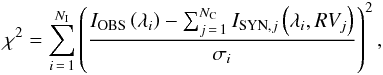 (1)where IOBS is the observed spectrum, ISYN,j the synthetic spectrum of the jth component, NI is the number of discrete elements of the digitised spectrum, NC is the number of the components of the system, RVj is the radial velocity of the jth component, and σi the standard deviation of the ith point of the observed spectrum, which was estimated from the continuum and adopted for the whole spectrum.
The majority of the spectra at our disposal was acquired in three wavelength regions Δλ∈{ 4200−4500;4750−5000;6200−6700 } Å. Each region contains a Balmer line, which turned out to be the best for measuring the RVs of component B and several metallic lines, which gave accurate RVs of components Aa and Ab. These regions were also extracted from echelle spectra, and RVs were measured on each region independently. The last region (Hα) contains a number of telluric lines, including the Hα line itself. Our model is unable to account for a telluric spectrum, and consequently it was not possible to measure accurate RVs of Hα with this technique.
Journal of the spectro-interferometric observations.
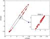 |
Fig. 1 Coverage of orbits 1 and 2 with the spectro-interferometric observations. The outer plot: the black line denotes the orbit of the centre of mass of the eclipsing binary relative to component B (which resides at the beginning of the coordinate system of the outer plot), and red dots denote the relative position of the centre of mass of the eclipsing binary relative to component B at the epochs of spectro-interferometric observations. The inset plot: the black line denotes the orbit of component Ab relative to component Aa (which resides at the beginning of the coordinate system of the inset plot), and red dots denote the relative position of component Ab relative to component Aa at epochs of spectro-interferometric observations. In both plots the orbital elements are invariable, i.e. they do not show the true orbits 1 and 2 as they would appear on the sky, but only demonstrate that the spectro-interferometric observations sample the orbits well enough to constrain elements of both orbits. |
Initial RVs for the searching program were computed from the orbital solution presented in Nemravová et al. (2013), and we searched for the RV for each component in the interval [− 70;70] km s-1 that surrounds the initial estimate. The components of the eclipsing binary Aa and Ab are very similar, therefore we had to verify that the two components had not been interchanged by the program, especially near the conjunctions. If they were, the search was repeated using a narrower search interval.
The RVs and their uncertainty were estimated in the following way:
-
1.
The parameters of synthetic spectra were chosen randomlyfrom the Gaussian distributions centred at values listed inTable 7, and the standard deviations were set totheir uncertainties.
-
2.
The synthetic spectra were fitted to the observed ones. The procedure was repeated five hundred times for each spectrum, and the RV including its uncertainty was estimated from the resulting distribution.
This approach allowed us to estimate only the statistical part of the total uncertainty. The statistical uncertainty ΔRVstat was typically ≤ 1 km s-1 for components Aa and Ab and ≤ 10 km s-1 for component B. Measuring the RVs of component B was more difficult because the majority of metallic lines in its spectrum is very shallow and smeared out by the high rotational velocity of component B. The measurements are also very sensitive to the choice of the model and its discrepancies.
The telluric lines in the red and IR parts of the spectra were used to correct for the variations of the zero-point of the RV scale. These corrections were typically ≤ 2 km s-1 for the Ondřejov spectra, hence all measurements for which the RV zero-point could not be checked in this way were assigned an uncertainty max(ΔRVstat,2) km s-1, and the remaining ones were assigned an uncertainty max(ΔRVstat,1) km s-1, where 1 km s-1 is the upper bound of the precision of the zero-point correction for the Ondřejov spectra.
3.2. Direct analysis of RVs
Since we were not aware of any publicly available program for orbital solutions of hierarchical systems with apsidal advance of the outer orbit(s), JN developed such a program. The measured RVs were fitted with a model, which takes into account the two dynamical interactions between the three or four components. The effects considered are the apsidal motion of orbit 2 and the light-time (LITE) effect produced by orbits 2 (ΔtLITE ≲ 0.006 d) and 3 (ΔtLITE ≲ 0.013 d). The RVs of the jth component RVj were fitted with the standard Keplerian model: ![\begin{eqnarray} RV_{j}(t) = \sum_{i}^{} K_{i}\left[\cos\left(\omega_{i}(t)+v_{i}(t)\right) + e_{i}\cos{\omega_i(t)}\right], \label{eqSpectroscopyRV} \end{eqnarray}](/articles/aa/full_html/2016/10/aa28860-16/aa28860-16-eq56.png) (2)where the index i goes over those orbits of ξ Tau that are relevant for the motion of the jth component of the ξ Tau system, Ki is the semiamplitude of the RV curve, ωi the argument of periastron, vi the true anomaly, ei the eccentricity, and t is time. The LITE ΔtLITE was computed using the following formulae:
(2)where the index i goes over those orbits of ξ Tau that are relevant for the motion of the jth component of the ξ Tau system, Ki is the semiamplitude of the RV curve, ωi the argument of periastron, vi the true anomaly, ei the eccentricity, and t is time. The LITE ΔtLITE was computed using the following formulae: ![\begin{eqnarray} \Delta t_{\rm LITE,j}(t)=\sum_{i}\frac{P_{i}K_{i}\left(1-e_{i}^{2}\right)^{\frac{3}{2}}}{2\pi c}\frac{\sin\left[\omega_{i}(t)+v_{i}(t)\right]}{1+e_{i}\cos v_{i}(t)}, \label{eqSpectroscopyLITE} \end{eqnarray}](/articles/aa/full_html/2016/10/aa28860-16/aa28860-16-eq63.png) (3)where the index i goes over those orbits that are hierarchically above the orbit in which the jth component lies (i.e. over those that produce LITE), P is the orbital period, and c is the speed of light. Otherwise the notation is the same as for Eq. (2). The argument of periastron is a linear function of time
(3)where the index i goes over those orbits that are hierarchically above the orbit in which the jth component lies (i.e. over those that produce LITE), P is the orbital period, and c is the speed of light. Otherwise the notation is the same as for Eq. (2). The argument of periastron is a linear function of time 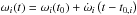 , where t0,i is the reference epoch and
  is the mean apsidal motion of the ith orbit.
The model elements were optimised by searching the minimum of the following χ2: ![\begin{eqnarray} \chi^{2}=\sum_{k\,=\,1}^{N_{\rm S}}\sum_{j\,=\,1}^{N_{\rm C}}\sum_{l\,=\,1}^{N_{\rm O}}\frac{1}{\sigma_{j,l}^2}\left[RV_{j}^{\rm OBS}(\tilde{t}_{j,l})-RV^{\rm SYN}_{j}\left(\tilde{t}_{j,l}\right)-\gamma_{k}\right]^{2}, \label{eqSpectroscopyChi2} \end{eqnarray}](/articles/aa/full_html/2016/10/aa28860-16/aa28860-16-eq68.png) (4)where the index k goes over NS subsets of the measured RVs, which are defined in Table 2, the index j over NC components of the ξ Tau system for which RVs were measured, and the index l goes over NO individual measurements of the RV and
(4)where the index k goes over NS subsets of the measured RVs, which are defined in Table 2, the index j over NC components of the ξ Tau system for which RVs were measured, and the index l goes over NO individual measurements of the RV and  is time corrected for the LITE. σ denotes individual rms of the RVs estimated with the procedure described in Sect. 2, RVOBS the measured RV, RVSYN the model RV computed with Eq. (2), and corrected for the LITE via Eq. (3), and γ denotes the systemic velocity. The minimum of the χ2 given by Eq. (4) was searched for with the sequential least-squares routine (Kraft 1988).
As discussed above, RVs of component B are less accurate than those of components Aa and Ab. Hence only RVs of the members of the eclipsing binary were fitted to obtain the majority of orbital elements. The individual subsets for individual types of the spectra gave very similar values of the systemic velocity (within 3σ), hence all available measurements were grouped together and a joint systemic velocity was derived for them. When a final solution was obtained, the measurements were complemented with RV measurements of component B and the mass ratio q2 was optimised (keeping the remaining parameters fixed). The parameters corresponding to the best-fit solution are listed in Table 5. RVs and the best-fitting model are plotted against time (to show the secular evolution of the periastron argument) for orbit 2 in Fig. 2, and against phase for orbit 1 in Fig. 3.
The uncertainties and correlations of individual parameters were estimated with the bootstrap method. One thousand samples were randomly chosen from all available RVs. Each sample consisted of the same number (748) of measurements as the original (meaning that some measurements repeat within a sample). Each sample was fitted with an orbital model and the uncertainties were estimated from the distribution of the results.
The reduced χ2 (denoted  throughout the article)
  , which is greater than ideal case of 1, is probably caused by variations of the RV zero-point larger than we accounted for (we note that the estimate is based on the variations of the zero-point measured on the Ondřejov red spectra), and by the fact that the synthetic spectra need not correspond to the observed ones in all details, for which we cannot account properly. Moreover, the model does not account properly for the dynamical interaction (see Sects. 8 and 9) between all orbits.
We also fitted a model including orbit C fixed at the orbital elements given in Table 10. The reduced χ2 was only marginally (≤ 1%) lower than that in Table 5. This is expected because the semi-amplitude of the RV caused by the revolution of the triple subsystem around the common centre of gravity with component C is ≈ 1 km s-1 and the LITE produced by that motion is ≈ 0.013 d, which means that both are beyond the detection limit of our measurements.
 |
Fig. 2 RVs of the centre of gravity of the eclipsing binary (red triangles) and component B (blue triangles) against the best-fitting model (black) corresponding to parameters listed in Table 5. ΔAa,Ab (in km s-1) denote residuals of the fit for RVs of the centre of gravity of the eclipsing binary, and ΔB (in km s-1) residuals of the fit for RVs of component B. |
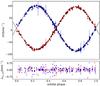 |
Fig. 3 RVs of components Aa (red) and Ab (blue) relative to the centre of gravity of the eclipsing binary against the best-fitting model (black) listed in Table 5. ΔAa,Ab are residuals of the fit for components Aa and Ab. |
3.3. Spectral disentangling
We were only able to separate the spectra in the vicinity of five major spectral lines Hα, Hβ, He i 4471 Å, Mg ii 4481 Å, and Hγ because only these regions were available for both the slit and echelle spectra. An attempt was made to separate the spectra of individual components using only the spectra from the three available echelle spectrographs. However, these separated spectra had strongly warped continua and were unsuitable for further investigation.
We used the program KOREL(Hadrava 1995, 1997, 2009) (release 04-2004), which not only separates the spectra, but also fits the spectroscopic orbital elements. This gave us the opportunity to compare the orbital solution obtained directly from the measured RVs with the result of KOREL. Only components B, Aa, and Ab were fitted because component C is not detectable. Relative luminosities of all three components were kept constant during the orbital motion. This assumption, although not exactly satisfied because of the shallow eclipses of components Aa and Ab, was necessary for the stability of the disentangling.
The orbital elements presented in Table 5 served as the starting estimates for the minimisation. The spectroscopic orbital elements obtained with KORELare listed in Table 6. The separated profiles from the considered spectral regions are shown in Fig. A.1. KORELdoes not provide the uncertainties of the fitted elements. Therefore a map of the χ2 around the minimum found with the minimisation engine was drawn for every combination of two fitted parameters. The uncertainties, which are listed in Table 6, correspond to 68% confidence intervals (roughly one σ) estimated from these maps.
Orbital elements obtained by KOREL(spectral disentangling) for all available spectra containing at least one of the studied regions.
An attempt was carried out to separate the lines of component C within two spectral bands in the near infrared, ΔλIR = { 7750−7800,8570−8800 } Å. The spectrum of component C was not detected in either of these bands. It was probably caused by the relatively low signal-to-noise ratio (S/N) of the echelle spectra in the infrared region and their limited number.
We also note that we tried to use the separated profiles instead of synthetic ones to measure RVs with the PYTERPOL program written by JN. This worked well for components Aa and Ab, but failed for component B. The reason is that the shape of the separated spectral lines depends on the orbital elements, for which the spectra were separated, and vice versa. Hence the separated spectra partially “remember” the orbital elements for which they were obtained, and if they are used for the RV measurements, they would give a fine RV curve described by a solution close to these elements. This becomes a problem when one or more orbital elements suffer from a large uncertainty, which was the case for ξ Tau in the mass ratio of orbit 2.
3.4. Comparison of observed and synthetic spectra
JN has developed a Python program PYTERPOL2, which interpolates in a pre-calculated grid of synthetic spectra to obtain estimates of the radiative properties of the components of multiple systems. For ξ Tau these parameters were the effective temperature Teff, gravitational acceleration log g, the projected rotational velocity vsini, RV, and the relative luminosity LR. The parameters of components Aa, Ab, and B were covered by the POLLUX grid (Palacios et al. 2010), and component C was searched for using the AMBRE grid (de Laverny et al. 2012). Solar metallicity was assumed.
The fit was carried out in four spectral regions, but only three relative luminosities were derived, since two of the regions are very close to each other and the luminosities LR are most likely almost the same.
The spectral regions were Δλ1 = [4280,4495] Å, Δλ2 = [4815,4940] Å, and Δλ3 = { [6330,6390];[6660,6695] } Å.
The relative luminosities were assumed to be constant over each spectral region Δλi.
Two of the regions contain a Balmer line, which constrains the gravitational acceleration of all three components, and also a large number of metallic lines, which constrain the temperature, RVs, and the projected rotational velocities. We fitted 137 spectra from the Ondřejov Observatory together because their normalisation is straightforward (a first-order polynomial often suffices to fit the continuum), so that the Balmer lines are not affected by systematics often introduced by the normalisation. The uncertainty of the relative flux was estimated from the continuum for each spectrum and set constant for each spectrum.
The bootstrap method was used to obtain a best-fit set of parameters. We randomly drew 137 spectra from the pool of 137 Ondřejov spectra (meaning that one or more spectra can be present multiple times within the random sample) and fitted them. The initial set of parameters was randomly chosen from intervals3 which were established from the first trial fits. The initial RVs were estimated from the orbital solution presented in Nemravová et al. (2013) and randomly put slightly off (within 30 km s-1 vicinity of the estimate) to secure robustness of the final solution. The procedure was repeated five hundred times and the final set of parameters was estimated from the distribution of the results. The shape of the distribution was Gaussian-like, that is, describable with a mean value and its standard deviation. The results are presented in Table 7.
Parameters of the fit of the synthetic spectra to 137 observed Ondřejov spectra.
A comparison of four spectral regions with the model is shown in Fig. 4. The reduced is lower than one, indicating that we have slightly overestimated the uncertainty of the relative flux of the observed spectra.
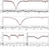 |
Fig. 4 Example of the fit of the synthetic spectra (red) to three observed spectra (black) in spectral regions: 1) Δλ1 = [4280,4495] Å (top), 2) Δλ2 = [4815,4940] Å (middle), 3) Δλ3 = [6330,6390] Å (bottom, left), 4) Δλ3 = [6660,6695] Å (bottom, right). The synthetic spectra are given by parameters listed in Table 7. |
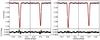 |
Fig. 5 Fit of the light curve from the satellite MOST. Only the light curve minima and their surroundings are shown. The primary (secondary) minimum is on the left (right) on each panel. The left panel corresponds to the global circular solution e1 = 0.0 and to orbital period P1 = 7.14664 d. The right panel corresponds to a local solution, where small adjustment of the eccentricity and the orbital period was allowed. MO denotes the satellite broad-band filter. |
3.5. Comparison of synthetic and separated spectra
We fitted the separated spectra corresponding to the solution of Table 6 with the interpolated synthetic spectra to check the results of Sect. 3.4. The program PYTERPOL was used again. The following spectral regions were fitted:
![\begin{eqnarray*} && \Delta\lambda_1=\lbrace{\left[4280,4400\right]; \left[4455,4495\right]\rbrace}~\r{A}, \\ && \Delta\lambda_2=\left[4765,4970\right]~\r{A},~{\rm and} \\ && \Delta\lambda_3=\lbrace{\left[6325,6395\right]; \left[6510,6620\right]; \left[6655,6695\right]\rbrace}~\r{A}. \end{eqnarray*}](/articles/aa/full_html/2016/10/aa28860-16/aa28860-16-eq123.png) The parameters corresponding to the best-fitting synthetic spectra are listed in Table 8. The best-fit parameters were estimated with a MCMC simulation and the uncertainties reflect only the statistical part of the uncertainty. The systematic uncertainty – the warp in the continua and the need for its normalisation – cannot be easily quantified and is responsible for the extremely high reduced along with the very high S/N ratio of the separated spectra. Therefore the uncertainties of the parameters listed in Table 8 are very likely underestimated.
The parameters corresponding to the best-fitting synthetic spectra are listed in Table 8. The best-fit parameters were estimated with a MCMC simulation and the uncertainties reflect only the statistical part of the uncertainty. The systematic uncertainty – the warp in the continua and the need for its normalisation – cannot be easily quantified and is responsible for the extremely high reduced along with the very high S/N ratio of the separated spectra. Therefore the uncertainties of the parameters listed in Table 8 are very likely underestimated.
Parameters of synthetic spectra best-fitting the separated spectra.
This systematic effect corrupts the estimate of log g of all components, especially component B, where the warping was the most pronounced; therefore it also applies to the rotational velocity of component B. The rotational velocity of components Aa and Ab is strongly affected by the choice of the instrumental broadening, which is very difficult to estimate for separated spectra and was set to 0.2 Å. The total light is also very likely affected by the re-normalisation, which (necessarily) changes the depths of spectral lines ( for all studied bands).
Bearing all this in mind, we state that this result does not contradict, but rather supports that obtained by fitting of synthetic to observed spectra. A comparison of the synthetic spectra corresponding to the parameters listed in Table 8, of separated spectra, and of re-normalised separated spectra is in Fig. A.1.
4. Photometry
The preliminary analysis published in Nemravová et al. (2013) has shown that the light variations can be attributed to the eclipses of components Aa and Ab of orbit 1. They partially eclipse each other and produce two very narrow and nearly identical minima, which are only ≈ 0.1 mag deep in the Johnson V passband.
In addition to the binary eclipses, our new very precise MOST satellite observations unveiled persistent low-amplitude rapid cyclic light changes that are probably associated with component B, since they remain during both binary eclipses. The MOST light curve also allows determining very accurate radii of components Aa and Ab as well as detecting variations of the mean motion of the eclipsing pair. The zoomed parts of both minima of the MOST light curve are shown in Fig. 5.
4.1. Period analysis of the light curve
Our first goal in the analysis of the MOST light curve was to unveil the nature of the rapid cyclic low-amplitude changes. Two different methods were used to construct and investigate the periodogram of the light curve. The first is based on the Fourier transform (FT hereafter) and is implemented in the program PERIOD04 (Lenz & Breger 2004). The second uses the phase dispersion minimisation technique (PDM) (Stellingwerf 1978) and is implemented in the program HEC274. The periodogram of the whole light curve is dominated by the orbital period of the eclipsing binary P1 ≈ 7.147 d. To study the rapid low-amplitude oscillation, we removed the eclipses (see Fig. 7, top).
The periodogram of the rapid oscillations (see Fig. 6) shows a basic frequency of f0=2.38d-1, most likely due to rotation of component B, the first harmonics of the eclipsing binary orbital frequency f1=2 /P1=0.279d-1; the frequencies of fd=1.002738 d-1 and fMOSTorbit=14.2 d-1 are instrumental (i.e. the orbital frequency of the satellite). The remaining prominent frequencies falias= {15.1734, 17.5385, 28.3896, 42.5825, 56.7745, 70.9720} d-1 seem to be either integer multiples of forb or its splittings with f0 or fd. Remaining peaks (e.g. f = 87.1609 d-1) have relatively low S/N ratios. We are not aware of any instrumental effect that would induce oscillations at f0 = 2.38d-1, hence the low-amplitude variations arise from a physical process in ξ Tau.
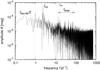 |
Fig. 6 Fourier spectrum of the MOST light curve from Fig. 7 (i.e. outside eclipses). Prominent frequency peaks are marked (see their description in Sect. 4.1). |
A closer look at Fig. 7 shows that the amplitude of the curve varies. To quantify these changes, a harmonic function f(t) = 1 + C0 + A0sin [ 2π(t−T0)f0 + φ0 ] was sequentially fitted to segments of the light curve Δt1 = P1/ 2 d wide, and shifted with a step Δt2 = P1/ 20, where P1 is the period of the eclipsing binary. The scan revealed that both the basic frequency f0 and its amplitude A0 vary on the time span of two orbital periods of the eclipsing binary (see Fig. 7, middle and bottom panels).
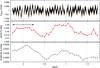 |
Fig. 7 Normalised light curve as reduced from MOST photometry, but without intervals of primary and secondary eclipses (top panel), together with the corresponding period P0 (middle) and amplitude A0 (bottom) of the harmonic function f(t) = 1 + C0 + A0sin [ 2π(t−T0) /P0 + φ0 ], which was sequentially fitted to the light curve, always in limited intervals ΔE1 = 0.5 of the epoch (indicated by the black double arrow), shifted with a step ΔE2 = 0.05. The oscillations exhibit both frequency and amplitude modulations, with periods spanning P0 = (0.42 ± 0.01) d and amplitudes A0 = (0.00060 ± 0.00015) mag. It seems that the longest P0 and the largest A0 are observed at around primary eclipses and vice versa. |
4.2. Nature of quasiperiodic oscillations
The quasiperiodic oscillations clearly visible in the MOST light curve with an approximate period P0 ≃ (0.42 ± 0.01) d and an amplitude A0 = (0.00060 ± 0.00015) mag exhibit both a frequency (FM) and an amplitude modulation (AM) on the time span of about the two shortest orbital periods P1 (see Fig. 7). We can think of several possibilities regarding their origin: an instrumental effect, a fifth component and ellipsoidal variations, rotation with spots, or rotation and pulsations.
The first option does not seem very likely, however, because we do not know about any instrumental period of 0.42 d (like one day, or a satellite orbital period 0.07042 d in this case).
A hypothetical fifth component (second option) orbiting either component B, Aa, or Ab with a period 2P0 can induce ellipsoidal variations of the order of A0, but they would be expected to be very regular (without large AM, FM) and to manifest themselves in one of the RV curves as well, which is not the case. We do not see any peak in the Fourier spectrum at f0 = 1 /P0 = 2.38 d-1, even though the Nyquist frequency for our spectroscopic dataset is fNy = 7.1 d-1. Nevertheless, the coverage and cadence are not uniform at all and the expected amplitude is small (5 km s-1), which makes this particular argument weak. We would also expect to see some frequency modulation due to the (classical) Doppler effect,  , with v ≃ 2vkepl. However, for 0.423 d we would only obtain a change by 0.001 d, which is one order of magnitude smaller than the observed total variation.
The lower limit for the rotation period is the critical rotation, Pmin = 2π(GM/R3)− 1 / 2, and the upper limit is determined by rotational broadening, Pmax = 2πR/ (vsini) (cf. Table 8). For component Aa or Ab, the admissible range is from about Prot = 0.180 d to 3.85 d, for component B it is 0.325 to 0.634 d. The observed oscillations are within both ranges, so that we cannot distinguish the source component at this point. One can argue that small axial inclination for components Aa, Ab is unlikely when their orbital inclination is large, so that their true Prot>P0. We thus prefer to attribute these oscillations to component B. Additionally, this star is relatively brighter so that it is easier to induce the oscillations of given amplitude A0.
It seems difficult to distinguish between spots and pulsations (options three and four above; as in Degroote et al. 2011). Especially for early-type stars, spots are infrequent, unless a star is chemically peculiar or magnetically active (Bp), but we have no observations and analyses at our disposal that could prove or disprove this for ξ Tau.
Pulsating B stars (like β Cep, SPB) always exhibit a low-frequency signal corresponding to the rotation and then a series of pulsation modes, either pressure (high-frequency) or gravity (low-frequency). The cadence of MOST photometric observations allows us to compute the Fourier spectrum up to fNy = 719 d-1, corresponding to 0.00139 d = 2 min (Fig. 6). Except for the basic rotational period, its aliases with the orbital period P1 of the eclipsing binary, one-day and Porb instrumental periods, we can unfortunately not unambiguously detect any pulsation modes with S/N≥5, to say nothing about rotational splittings, which would be conclusive.
4.3. Eclipse timing variations
The orbital period of the eclipsing binary P1 = 7.14664 d introduces a small but clearly detectable shift ΔPHASE ≈ 0.0003 between the two minima recorded with the MOST satellite. The shift disappears if the orbital period and the eccentricity are optimised. The local period and eccentricity, which do not cause the phase shift, are P1 = 7.14466 d and e1 ≃ 0.002. The problem is illustrated in Fig. 5, where the comparison of an eccentric model with the local value of the orbital period and a global circular model is shown. An even larger phase shift Δp ~ 0.004 was detected when a similar analysis was carried out for all photometric observations.
This led us to investigate the eclipse timing variations (ETVs) in all available photometry, divided into subsets covering time intervals shorter than P2/ 4 (individual minima are shown in Figs. B.1 and B.2). The ETVs are very noisy, and the delays themselves have an amplitude ΔtOBS ≈ 0.025 ± 0.01 d that cannot be explained by LITE (ΔtLITE ≲ 0.006 d). Moreover, they seem to vary on a timescale comparable to the orbital period P2. Hence we assume that the dynamical interaction between orbits 1 and 2 is the reason for these delays. The first-order model of the physical delay (Eq. (8) from Rappaport et al. 2013), which is only a part of the total ETV, arising from dynamical interaction of two orbits in hierarchical triple systems, gives an estimate of the amplitude of the effect ΔtMODEL ≈ 0.02 d, (i.e. in rough agreement with the detected value). This is another proof of the dynamical interaction in ξ Tau (the first is the apsidal motion reported by Nemravová et al. 2013) and led us to develop an N-body model (see Sect. 8) and a perturbation theory (see Sect. 9).
4.4. Global orbital model for all light curves
The program PHOEBE1.0 (Prša & Zwitter 2005, 2006) was used to derive the light-curve solution. The mass ratio q1 was taken from the analysis of the RVs (see Table 5) because only light curves were modelled and they do not constrain the mass ratio for a detached system. The eccentricity was assumed to be e1 = 0.0 (although Sect. 8 shows that orbit 1 is slightly eccentric). The value of the semi-major axis a was adjusted after each iteration based on a1sini given by the fit of the directly measured RVs (see Table 5). The linear limb-darkening law was adopted and the coefficients were interpolated in a pre-calculated grid distributed along with PHOEBE. The bolometric albedos were taken from Claret (2001) and the gravity brightening coefficients from Claret (1998) for the corresponding temperatures of components of the eclipsing binary. The spin-orbit synchronisation, that is, the synchronicity ratios FAa = FAb = 1, was assumed, because radii RAa and RAb from Nemravová et al. (2013) and rotational velocities from Table 7 give synchronicity ratios FAa = 1.12 ± 0.26, and FAb = 0.74 ± 0.20; the deviations from the corotation are small and probably arise from an incorrect determination of the radii. The primary effective temperature  was set to the value found through a comparison of synthetic and observed spectra.
The orbital inclination i1, Kopal surface potentials  of both components and the epoch of the primary minimum Tmin,1, the secondary temperature , and the relative luminosity of component B
  in each spectral band were optimised. Initial estimates of these parameters were taken from Nemravová et al. (2013), initial relative luminosities
  of component B were estimated from the comparison of synthetic and observed profiles (Table 7). The primary luminosities
  were adjusted after each iteration.
The fitting was carried out in the Python environment of PHOEBE, and the minimum was determined with the differential evolution algorithm (Storn & Price 1997). The following parametric space was searched: Tmin,1 ∈ [56 224.68,56 224.78] RJD, i1 ∈ [84,90] deg, ![\hbox{$\Omega^{\rm Aa}_{\rm K} \in \left[11, 20\right]$}](/articles/aa/full_html/2016/10/aa28860-16/aa28860-16-eq213.png) ,
, ![\hbox{$\Omega^{\rm Ab}_{\rm K} \in \left[11, 20\right]$}](/articles/aa/full_html/2016/10/aa28860-16/aa28860-16-eq214.png) ,
, ![\hbox{$T_{\rm eff}^{Ab} \in \left[10\,000, 10\,700\right]$}](/articles/aa/full_html/2016/10/aa28860-16/aa28860-16-eq215.png) K, LB ∈ [0.55,0.78]. The last interval applies to each studied spectral filter (U, B, V, MOST). The parametric space was densely sampled with models during the fitting (≈ 300 000 light curve models were computed). This showed that the relative luminosity of component B LB is poorly constrained.
K, LB ∈ [0.55,0.78]. The last interval applies to each studied spectral filter (U, B, V, MOST). The parametric space was densely sampled with models during the fitting (≈ 300 000 light curve models were computed). This showed that the relative luminosity of component B LB is poorly constrained.
After a global minimum was found, we split our data and optimised the ephemeris, relative luminosity of component B, and surface potentials using only observations from the MOST satellite, after which we optimised the effective temperature of component Ab and the relative luminosity of component B using the Johnson UBV photometry. The epoch of the primary minimum was also fitted for the UBV dataset to slightly adapt it for the ETVs discussed in Sect. 4.3.
The parameters corresponding to the best-fitting model are listed in Table 9. Our model is unable to account for either the rapid light oscillations or the ETVs; therefore we raised the uncertainty of observations from the MOST satellite to deal with the former (ΔmMOST = 0.006 given by the sinusoidal fit). The uncertainties of parameters are estimated as 68% confidence intervals computed from a scaled χ2 (scaled to an ideal situation, where the  ), although in this case the scaling was almost unnecessary, since the best solution has
  .
.
Parameters of the best-fitting circular orbital model obtained with the program PHOEBE 1.0.
5. Astrometry of orbit 3
We used the existing astrometric positions listed in the WDS catalogue (see Mason et al. 1999, and references therein) to improve the orbital elements of orbit 3 published by Rica Romero (2010). The solution was carried out with the help of the program written by PZ (see Zasche & Wolf 2007, and references therein). The solution is listed in Table 10 and the orbit is shown in Fig. 8.
Orbital elements of orbit 3 based on a fit to astrometric measurements published in WDS.
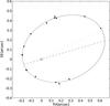 |
Fig. 8 Speckle-interferometric outer orbit 3 corresponding to the solution of Table 10. The dotted line stands for the line of apsides, the dashed line for the line of nodes. |
6. Spectro-interferometry
In this section we present an orbital analytic model of the ξ Tau system, which we fit to spectro-interferometric observations to estimate orbital elements, radii, and fractional luminosities of ξ Tau.
6.1. Global model for all available spectro-interferometric observations
The calibrated visibilities from VEGA/CHARA were fitted night by night with a model consisting of three uniform disks using the tool LitPro5 (Tallon-Bosc et al. 2008). The observations obtained during each single night were not numerous enough to safely estimate the positions and radii of components Aa, Ab, and B on the celestial sphere. In contrast to this, the NPOI observations are numerous enough to provide good estimates of the relative position of component B and the photocentre of the eclipsing binary for each night. They are presented in Table C.1 along with details on their acquisition (see Appendix C).
To circumvent the problem, we created a global orbital model that computes instantaneous positions of components B, Aa, and Ab with the following formulae:
 where index i denotes the component of a binary, v is the true anomaly, ω the argument of periastron, i the orbital inclination with respect to the celestial sphere, Ω is the position angle of the nodal line, a the angular semimajor axis, and e the eccentricity. The position angle αi is measured counter-clockwise from the north, ρi is the angular separation of a component, and the centre of mass, (xi,yi) is the same in Cartesian coordinates. The instantaneous value of the argument of periastron is given as follows:
  , where Tp is the reference periastron epoch and ω0 is the value of the periastron argument at the reference epoch. Instead of computing the semi-major axis for each component of a binary, the semi-major axis a and the mass ratio q = M1/M2 were used; the semi-major axes of primary and secondary can be computed with the following formulae: a1 = aq/ (1 + q), a2 = a/ (1 + q). The periastron argument of the secondary is ω2 = ω1 + π.
In our application of Eqs. (5)−(8) component B is fixed at the beginning of the coordinate system because the observations are only sensitive to relative positions of the stars, not to the system as whole.
When the positions of all three components are known, objects representing each component can be placed at these positions. The uniform disk was chosen because all three components are detached and therefore only minor departures from spherical symmetry can be expected. The squared visibility V2 and closure phase T3φ for such a model can be computed analytically with the following formulae:
![\begin{eqnarray} && \left|V_{{\rm S},k}({\vec f})\right|^{2} = \left|\frac{\sum_{j=1}^{N} L_{j,k}\frac{2J_{1}\left(\pi\theta_{j} B/\lambda_{k}\right)}{\pi\theta_{j} B/\lambda_{k}}e^{-2\pi i\left({\vec f}\cdot{\vec r}\right)}}{\sum_{j=1}^{N} L_{j,k}}\right|^{2},\label{eqInterferometryVisibility}\\ && T_3\phi_{{\rm S},k}({\vec f}_1, {\vec f}_2) = \arg\left[V_{{\rm S},k}({\vec f}_1)V_{{\rm S},k}({\vec f}_2)V_{{\rm S},k}(-{\vec f}_1 - {\vec f}_2)\right],\label{eqInterferometryClosurePhase} \end{eqnarray}](/articles/aa/full_html/2016/10/aa28860-16/aa28860-16-eq252.png)
where index j denotes a component of the triple system, k the spectral band, V the visibility, f = (u,v) the spatial frequency, L the luminosity fraction, B the length of the baseline, θ the diameter of the uniform disk, λ the effective wavelength (the central wavelength of the spectral band), J1 the first-order Bessel function,  the Cartesian coordinates of a component computed with Eqs. (5)−(8), and N the total number of components in the system. The uniform disk diameter θ is also a wavelength-dependent quantity, therefore a different radius should be derived for each spectral band. Nonetheless, the dependency is very weak (order of 10-3 mas for the whole wavelength span of our data).
6.2. Orbital solution for all available spectro-interferometric observations
The model given by Eqs. (5)−(10) was fitted to calibrated squared visibilities from all four instruments, that is, CHARA/VEGA, NPOI, MARK III, and VLTI/AMBER. The best-fit set of parameters was determined using the least-squares method, that is, by minimising the following χ2: 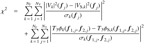 (11)where V2 (T3φ) is the observed squared visibility (the observed closure phase),
  (T3φS) the synthetic squared visibility computed with Eq. (9) (the synthetic closure phase, Eq. (10)), f = (u,v) the spatial frequency, σ the standard deviation of an observation, NV the total number of squared visibility observations, NT the total number of closure phase observations, and NF the total number of spectral bands.
The phase coverage of the inner and the outer orbits is good enough (see Fig. 1) to allow fitting of all orbital elements. Our strategy was to keep as many parameters free as possible, since this model is independent of those presented in Sects. 3 and 4. However, the angular size of the inner orbit is small and its ephemeris is obtained with greater precision by the photometry and spectroscopy. The eccentricity of orbit 1 was set to zero (see Table 5) because there were no signs of a significant eccentricity in previous analyses. A number of trial runs have shown that the inclination i1 and the mass ratio q1 are poorly constrained by the interferometric observations. If optimised, both converged to values not consistent with previous analyses (i1 ≈ 78 ± 5 deg, q1 = 0.8 ± 0.10). Investigation of χ2 maps surrounding these values has shown large shallow valleys that spread up to regions with values consistent with photometric and spectroscopic models. To stay on the safe side, we fixed both parameters at values obtained from the spectroscopy and photometry because they were estimated with much higher precision.
The global minimum of Eq. (11) was determined with the differential evolution algorithm (Storn & Price 1997) and was locally optimised with the sequential least-squares routine (Kraft 1988). The parameters of the best-fitting model are listed in Table 11. A large portion of the parametric space was searched6. The initial parametric space was equally sampled with a population which consisted of 1500 members. The population evolved until the mean energy of the population (i.e. the mean χ2 divided by its standard deviation and multiplied by the tolerance) was greater than one. The tolerance was set to 10-3 and the procedure took from 50 to 100 iterations to finish.
The final reduced  is much larger than 1 because the true uncertainty of the V2 derived with the reduction pipeline is underestimated. The reason is that the high is given mainly by data that were acquired at low spatial resolution and are expected to be easiest to reduce. Another reason is that the angular slit width of all interferometric instruments is comparable to the angular separation of component C and the triple, meaning that it cannot be guaranteed that it was recorded. The full amplitude of squared visibility variations caused by component C ranges from ≲0.035 in the V band to ≲0.050 in the K band. It introduces systematic errors that we cannot correct for. The last reason are imperfections of the model. We had to accept several simplifications to stabilise the fit. Uncertainties of the best-fit parameters were estimated at 68% confidence intervals from the scaled to one.
Several attempts have shown that we are insensitive to the diameters of components Aa and Ab, because we lack enough observations at very long baselines (reaching up to 300 m). If they were set free, the solution would converge to unrealistic values (≳ 1.0 mas), therefore they had to be fixed at values given by the parallax of the system and the light-curve solution (see Table 9). Convergence of the orbital parameters of orbit 1 was in general slow because the bulk of observations (NPOI, AMBER) was taken at low spatial resolution, at which this orbit is almost mainly on observations from VEGA/CHARA.
Our model allows fitting separate sets of relative luminosities LR for each passband because the visibilities were estimated in narrow passbands: four for CHARA/VEGA, sixteen for NPOI, and ≈ 40 for VLTI/AMBER. It was not possible to divide the data into a larger number of small groups and to densely sample the relative luminosity of components Aa, Ab, and B as a function of the wavelength. After a set of trial attempts, we split the data into two subsets: visible (MARKIII, NPOI, CHARA/VEGA) and infrared (AMBER). This sampling is justified by the very low variability of the luminosity ratios with wavelength of all stars within the visible and infrared regions, which we checked using synthetic spectra from the PHOENIX grid (Husser et al. 2013). The relative luminosities of components Aa and Ab did not converge to plausible values for the infrared subset (it generally predicted a too low luminosity ratio between the two components of orbit 1), therefore we decided to use the estimate based on the PHOENIX grid and radii obtained from the light-curve analysis for components Aa and Ab, and the radius of component B was taken from Harmanec (1988).
The best-fit set of parameters is listed in Table 11 and a plot of the model vs. the observations is shown in Figs. C.1−C.10. The model qualitatively fits the variations of the V2 (i.e. the curvature of the model data agrees with the curvature of the observed V2) for all spectro-interferometric data very well.
Summary of parameters derived from the spectroscopic, photometric, and spectro-interferometric analyses.
7. Summary of analyses based on simple analytic models
Here we critically compare the results of individual observational methods and derive the properties of the system.
7.1. Performance of different observational methods
Despite the subtitle, the individual models we used to evaluate different observational methods were not completely independent because the results from one method often served as a starting point for another. In some cases it was mandatory to take a parameter value from another model to stabilise the convergence to a steady solution. In the following paragraphs we discuss the outcome of different methods and their accuracy. An overview of all fitted parameters is given in Table 12 obtained through different methods (i.e. more values are given for some parameters). Corresponding properties of the orbits and stars are also listed. Orbital elements of orbit 3 are not listed because their properties were constrained only by astrometry, and they are presented separately in Table 10. The mass of component C is briefly discussed here.
-
The spectroscopic elements: elements (K, e, Tp, P, ω,
 ) of both orbits are estimated better from the fit of directly measured RVs with an analytic model (see Table 5, Eqs. (2) and (3)). The spectral disentangling works with a much more complex model, and the resulting orbital elements depend on the shape of the separated profiles (and vice versa), which come out warped (the degree of the warp is shown by grey line in Fig. A.1). The warp is most pronounced for component B, meaning that especially the mass ratio q2 coming from the method cannot be trusted. On the other hand, the thin lines of components Aa and Ab constrain the RVs very well even if the separated spectrum is not perfect, and for the remaining orbital parameters the disentangling therefore provides values that agree with the fit of directly measured RVs.
 -
The ephemeris of orbit 1: the photometric solution presented in Table 9 yields the best ephemeris (Tmin,1, P1) of orbit 1 especially thanks to high-precision observations from the satellite MOST. The ephemeris for orbit 1 estimated from the RVs does not agree within uncertainties with the photometric one. It can be caused by the lower precision of RV measurements around eclipses.
-
The eccentricity of orbit 1: it was set to zero throughout the analyses because the precision of data does not allow a reliable determination. The analysis of the light curve from the satellite MOST shows a hint of a small eccentricity, but the relative position of minima is also affected by ETVs, and we are unable to discern one from the other with the analytic models. The dynamics of the system (see Sects. 8 and 9) shows that the eccentricity should oscillate with an amplitude Δe ≈ 0.01. This introduces a jitter of the relative position of the primary and secondary minimum and increases uncertainty of the radii when a circular model is applied.
-
The inclination of orbit 1: it is determined accurately using the light-curve analysis presented in Table 9. The value obtained from the interferometric model suffers from large uncertainty and is about 10 deg off the photometric solution. This is probably caused by the low number of observations at high spatial frequencies and the calibration systematic errors, which are likely more pronounced for high-frequency data.
-
The longitude of the ascending node: the longitude of the ascending node of orbit 1 has a mirror solution Ω1 = Ω1 + 180 deg with (almost) the same value of the
, while the Ω2 is determined uniquely because the NPOI instrument acquired a large number of closure phase measurements. This means that it is not possible to say whether the motion of orbit 1 relative to orbit 2 is prograde or retrograde based solely on the spectro-interferometric data. -
The relative luminosities: they were determined from the light-curve solution, the comparison of synthetic and observed spectra, and from the interferometric solution.
-
The light-curve solution best describes their variations with thewavelength, but the values suffer from large uncertaintiesbecause of correlations between the fitted parameters.
-
The fit of synthetic spectra to observed ones is quite insensitive to relative luminosities, but this is the case only because small parts of red spectra were fitted that contain only three weak spectral lines. The relative luminosities obtained in the regions around Hγ and Hβ roughly agree with the values obtained for the B band from the light-curve solution.
-
The bulk of the interferometric observations falls somewhere between the V and R bands. Therefore the relative luminosities detected with the spectro-interferometry are close to the V-band value obtained from the light-curve solution. We were not able to obtain plausible estimates of relative luminosities for the infrared subset (AMBER) because the observations have low spatial resolution and do not resolve the eclipsing binary well.
-
The effective temperatures: they are given better by the fits of observed spectra to synthetic ones because the fitted regions contain many spectral lines (especially the region Δλ = [4280,4495] Å) where the photometry relies on four broad-band filters alone. In addition, Prša & Zwitter (2006) stated that it is not possible to obtain accurate effective temperatures of the two components of an eclipsing binary from the light-curve solution unless the colour-constraining method (described by them) is employed. According to the authors, the problem is even more pronounced when the two components are alike. Therefore we fixed the primary temperature and only optimised the secondary temperature. The result agrees with that obtained from the comparison of observed and synthetic profiles within the respective errors. The spectral types corresponding to these temperatures are B9 for components Aa and Ab and B5-6 for component B.
The semi-major axes and masses: the physical size of the semi-major axes derived from the spectro-interferometry and the Hipparcos parallax (orbits 1 and 2) and those derived from the spectroscopy and photometry (orbit 1) and spectroscopy and spectro-interferometry (orbit 2) agree with each other within their uncertainties. The same applies to masses, which seem to fall within the limits of normal main-sequence (MS hereafter) masses corresponding to the respective spectral types (Harmanec 1988) – mAa = 2.25 ± 0.03 ∈ [1.71,2.41]M⊙, mAb = 2.13 ± 0.03 ∈ [1.71,2.41]M⊙, mB = 3.89 ± 0.25 ∈ [3.63,4.6]M⊙.
The total mass of the system and mass of component C: using the parallax πa2 = 14.96 ± 0.51 and the solution presented in Table 10, we can estimate the total mass of the system mAa + Ab + B + C = 9.88 ± 1.06M⊙. A comparison with the masses of the inner triple subsystem gives an estimate of the mass of component C mC = 1.61 ± 1.18M⊙ that agrees with early F-type or late A-type star.
The component radii: all components seem to have normal radii for their respective spectral type (again checked against Harmanec 1988) – RAa = 1.70 ± 0.04 ∈ [1.40,2.06]R⊙, RAb = 1.62 ± 0.04 ∈ [1.40,2.06]R⊙, RB = 2.8 ± 0.3 ∈ [2.13,2.85]R⊙.
The dereddened colour index B-V: these are derived with a high level of uncertainty because of the high uncertainty in the luminosity ratios in different bands and the uncertainty of bolometric magnitudes. We compared the dereddened colour indices against tables computed by Flower (1996),
 K,
K,
 K, and
 K.
K.
They very roughly agree with the values found by the comparison of the observed and synthetic spectra. The uncertainty bars of the colour indices are very generous and match a wide range of temperatures.
The distance: the number of applied observational methods allows us to estimate the distance of ξ Tau from the ratio of the physical and angular size of the semimajor axes and from the distance modulus. The former seems to prefer parallax, which is slightly lower than the Hipparcos parallax (but still within error bars), the latter also places ξ Tau farther than the Hipparcos observations, but their uncertainties are large, meaning that they do not contradict the Hipparcos parallax. The parallax estimated from the ratio of the physical and angular size of the semi-major axis of the outer orbit yields the most precise parallax, πa2 = 14.96 ± 0.51 mas.
7.2. Conclusion of the analytic models
The spectroscopy, the photometry, and the interferometry were studied with traditional (semi-) analytic models. We found that results obtained from different methods are consistent with each other, although some of them give better estimates of a particular set of parameters than others. We took advantage of this differential sensitivity and compiled a resulting set of fundamental properties of the system.
During the analyses described in previous sections, we noted two effects that indicate the dynamical interaction in ξ Tau: the advance of the apsidal line of orbit 2, and the eclipse timing variations (ETVs) in system 1. The first effect was explicitly taken into account because omitting it would cause significant inconsistency between observations and model. The latter effect was almost overlooked if it had not been for the indication in the very accurate photometric data from the MOST satellite. However, the analytic models above give only limited insights into dynamical effects in a four-body system such as ξ Tau. Nonetheless, they provide very good results that are also needed as a starting point for a more sophisticated solution based on an approach that includes dynamical evolution in a more complete way. We proceed in two steps.
In Sect. 8 we develop a numerical model that consistently takes into account the gravitational interaction of all stars in the ξ Tau . We use a fully numerical implementation, basically a standard N-body integrator, which we extend by subroutines that allow us to model several types of observables relevant for the ξ Tau dataset.
Next, in Sect. 9 we summarise relevant analytic formulae obtained by methods of perturbation theory, which provide insights into results from the fully numerical approach in Sect. 8. Despite their limitations, we find the analytic formulation of the most important orbital perturbations useful. It does not only allow us to understand basic features in the numerical integrations, but also readily provides the parametric dependencies.
8. N-body model of ξ Tauri with mutual interactions
The quadruple nature of ξ Tauri and its relatively compact packing require us to proceed with an advanced N-body model that can account for mutual gravitational interactions of all four components. To this point, we now describe our numerical integrator, a definition of a suitable χ2 metric, and the overall results of our fitting procedure.
8.1. Numerical integrator and χ2 metric
We use a standard Bulirsch–Stoer N-body numerical integrator from the SWIFT package (Levison & Duncan 2013). Our method is quite general. We can model classical Keplerian orbits, of course, but also non-Keplerian orbits (involving N-body interactions). We treat all stars as point masses only, however. We have no higher-order gravitational terms and no tides in our model.
As explained below, this is a significant improvement of our previous application in Brož et al. (2010) because we can now account not only for the light-time effect, but for complete eclipse timing variations (ETVs) of the inner binary that arise from both direct and indirect gravitational perturbations. At the same time, we do not use the simplification of Brož et al. (2010) and consider all the components separately because the equivalent gravitational moment  (12)of the inner eclipsing binary Aa+Ab is large at the distance of the component B.
We used five different coordinate systems: (i) Aa-centric (to generally specify initial conditions and eclipse detection); (ii) barycentric (for the numerical integration itself); (iii) Aa+Ab photocentric (to compare with interferometric observations of component B); (iv) Aa+Ab+B photocentric (ditto for component C); and (v) Jacobian (to compute hierarchical orbital elements).
Initial conditions at a given epoch T0 can be specified either in Cartesian coordinates with x,y in the sky plane and z in the radial direction, or in osculating orbital elements. This very choice has a substantial role because the outcome of the fitting procedure will be generally (slightly) different. The orbital elements can be considered less strongly correlated quantities than Aa-centric Cartesian coordinates.
We accounted for as many observational data as possible using the following joint metric7:  (13)
(13) (14)
(14) (15)
(15)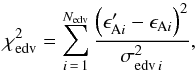 (16)
(16)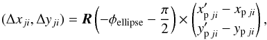 (17)
(17)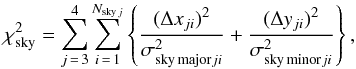 (18)where the notation is briefly described in Table 13. The dashed quantities are the model values linearly interpolated to the exact times ti of observations. The index j goes over the list of components Aa, Ab, B, C (i.e. j = 1 = Aa, ...), while the index i corresponds to the observational data.
Notation used for various coordinates, velocities, and uncertainties that we used in our N-body model.
In our N-body model we do not fit the observed spectra using synthetic ones, individual light curve points, or interferometric fringes. We use higher-level observational data instead that were reduced and derived in previous sections. Hence we fit RV measurements for the three components Aa, Ab, and B, altogether Nrv = 843, minima timings for the eclipses in the inner binary (Aa+Ab), Netv = 35, and astrometric observations for components B and C, Nsky = 49. The latter is a subset of measurements from NPOI and WDS, for which it was possible to convert fringe visibilities (averaged over one night) into distance–angle values. The individual uncertainties of the observations used in this section were modified as follows: σrv ≥ 2 km s-1 due to calibration uncertainties, σetv ≥ 0.001 d = 1.5 min because the quasi-periodic oscillations visible in the MOST light curve shift minima timings in a random fashion, and σsky = 3 mas (as in Tokovinin et al. 2015) or 5 mas if not reported in WDS.
We assumed the nominal distance d = 64.1 pc for ξ Tau. The stellar radii for an eclipse detection were RAa = 1.700 R⊙ and RAb = 1.612 R⊙, in agreement with the photometric inversion. The expected correlation among RAa, RAb, eclipse depth, eclipse duration and third light contribution is removed to some extent through spectroscopic observations (cf. Table 9).
The synthetic minimum distance Δ′ between components Aa and Ab in the sky plane was determined analytically as the distance of the piece-wise straight line (xAb,yAb) from the origin in the Aa-centric coordinates, as provided by the numerical integration. The condition for an eclipse is then Δ′ ≤ RAa + RAb and the corresponding time  is linearly interpolated from neighbouring points. The eclipse duration is then given by a simple geometry,
 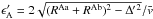 , where
  denotes the average velocity between the points. We thus straightforwardly account for disappearing eclipses and their durations, but we do not model (possible) eclipse depth variations at this stage.
To remove minor systematics in minima timings and eclipse duration, we attempted to suppress quasi-periodic oscillations visible in the MOST light curve by subtracting a function of the following form: ![\begin{eqnarray} f(t) &=& C_0 + C_1(t-T_1) \nonumber \\ & & -\, [A_0 + A_1(t-T_1)] \sin\left[{2\pi(t-T_1)\over P_0+P_1(t-T_1)}\right]\cdot \label{f_MOST} \end{eqnarray}](/articles/aa/full_html/2016/10/aa28860-16/aa28860-16-eq365.png) (19)Its coefficients (C0,C1,T1,A0,A1,P0,P1) were always determined by a local fit in the surroundings of the given minimum. The resulting data are reported in Table 14.
(19)Its coefficients (C0,C1,T1,A0,A1,P0,P1) were always determined by a local fit in the surroundings of the given minimum. The resulting data are reported in Table 14.
The relative luminosities for photocentre computations were set to LAa = 0.204, LAb = 0.174, and LB = 0.622, again in agreement with photometric observations.
Mass constraints also arise from the spectroscopic classification of the ξ Tau components (A9 V, A9 V, B5 V, and F V). We can easily enforce reasonable limits for the component masses with the following artificial term: ![\begin{equation} \chi^2_{\rm mass} = \sum_{j=1}^4 \left[ \left(m_j\!-\!{m_{j\,\rm min}\!+\!m_{j\,\rm max}\over 2}\right) {2\over m_{j\,\rm max}\!-\!m_{j\,\rm min}} \right]^{100}, \label{eq:mass_limit} \end{equation}](/articles/aa/full_html/2016/10/aa28860-16/aa28860-16-eq370.png) (20)where we used mAa and mAb∈ (0.9,3.0) M⊙, mB ∈ (3.5,3.9) M⊙, mC ∈ (0.9,2.0) M⊙ as the limits; the exponent is rather arbitrary.
(20)where we used mAa and mAb∈ (0.9,3.0) M⊙, mB ∈ (3.5,3.9) M⊙, mC ∈ (0.9,2.0) M⊙ as the limits; the exponent is rather arbitrary.
The integrator and its internal time step were controlled by the parameter ϵBS = 10-8 (unitless), which ensures a sufficient accuracy. The integration time span was 1000 d forward and 11 000 d backward, and the output timestep Δt = 0.5 d for initial runs. We verified that this sampling is sufficient even for the trajectory with the strongest curvature and all necessary interpolations to the times of observations. For the final optimisation we decreased the value further to Δt = 0.1 d to suppress interpolation errors.
We used a standard simplex algorithm (Press et al. 1993) to search for local minima of χ2. We have 23 potentially free parameters, masses mj, coordinates xj,yj,zj, velocities vxj,vyj,vzj in the Aa-centric frame, or, alternatively, masses mj and three sets of orbital elements aj,ej,Ij,Ωj,ωj,Mj in Jacobian coordinates, and the systemic velocity γ. The convergence tolerance for χ2 was set to ϵtol = 10-6, and the maximum number of iterations to 10 000 or to as low as 300 for extended surveys of the parameter space. We verified that this low number is sufficient to quickly detect local minima or to exclude their existence.
The initial epoch T0 = 2 456 224.724705 is very close to the first precise minimum of the MOST light curve. We can thus (almost) fix xAb ≃ yAb = 0. At the same time, it is possible to (approximately) fix positions xpB,ypB and xpC,ypC, derived by interferometry for an epoch close to T0.
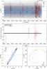 |
Fig. 9 One of the best-fit solutions for the ξ Tau system with our N-body model and using all available observational data. In this case, the resulting total χ2 is 2578, while the number of degrees of freedom ν = 908. Top: radial velocities vzbAa, vzbAb, vzbB, vzbC of the individual components; model values are denoted by lines (component Aa is black, not clearly visible, Ab grey, B blue, and C orange), observations by black error bars and residuals by thick red lines. Middle: O−C values for both primary and secondary minima timings; model timings are denoted by black points (very densely packed), observations by grey crosses, and O−C with its uncertainty by red error bars. Bottom left: astrometric positions of component B based on NPOI interferometric observations; model orbit xpB, ypB with respect to photocentre Aa+Ab (i.e. not w.r.t. B, as usually) is again denoted by a blue line, observations by black error bars and residuals by thick red lines. The orbit is not a single ellipse, but rather a complex trajectory that quickly precesses and is moreover affected by (slight) photocentre motions. Bottom right: similarly, astrometric positions of the distant component C xpC, ypC with respect to the Aa+Ab+B photocentre is denoted by an orange line. Component B is relatively luminous, which makes the orbit in these photocentric coordinates slightly jagged. |
8.2. Resulting best fits
As expected, the 23-dimensional parameter space is vast and full of local minima, even at high χ2. We proceeded sequentially to avoid complications and used a set with 2012 data only, a set with data from 2011–2013, and one set with all observational data. Next we performed a survey of the parameter space (to ensure we did not miss an obvious global minimum), an optimisation of individual orbits (2 and 3), the mutual inclination of orbits 1 and 2, and then we switched from Cartesian coordinates to orbital elements. Finally, we let all parameters be free. The optimisation means that we started the simplex from scratch many times (with different initialisation) and let it converge (for a limited number of iterations). Our largest survey consisted of 105 simplex runs, 300 steps each, that is, 3 × 10⁷ models in total, so that we are confident that there is no other hidden minimum, at least within the ranges searched so far8.
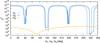 |
Fig. 10 Example of the one-dimensional χ2 mapping used to derive uncertainties of orbital elements for the ξ Tau system. The dependencies of the χ2 values on the three nodes Ω1, Ω2, Ω3 are shown, while the remaining elements correspond to the best-fit values from Table 15. The preferred solution for Ω1 ≃ 331°, with χ2 = 2578, and a hint of a mirror solution at Ω1 ≃ 151° are clearly visible. If the latter is optimised separately, we would obtain χ2 as low as 2 749. The sudden increase of |

Initial osculating orbital elements aj,ej,ij,Ωj,ωj,Mj of the ξ Tau system as derived by our N-body model.
We are aware of three mirror solutions (and 23 combinations), namely the inner binary can orbit in a retrograde or prograde sense with respect to orbit 2, so that  . Moreover, its node can be shifted by 180°,
  . Last but not least, orbit 3 can have the opposite inclination,
  (we have no direct RV measurements). These ambiguities are discussed and partly resolved in the following paragraphs.
Our best fit is presented in Fig. 9 and Table 15. We note that this is not the only fit that seems reasonable; there are many more available in the surroundings. This can be partially seen in Fig. 10 where one-dimensional χ2 maps exhibit relatively broad minima for the plotted parameters. Consequently, if we were to use simplex within these ranges, we would surely find a different minimum with slightly larger χ2 (or even slightly smaller).
We clearly see that the value of χ2 = 2578 is still about three times higher than the number of degrees of freedom, ν = Ndata−Mfree = 931−23 = 908, and formally speaking, we should be ready to admit that our model is plainly wrong. Nevertheless, the residua seem to be distributed normally, and realistic uncertainties (including some systematics) may be larger than expected. To obtain χ2 ≃ ν we would need measurement uncertainties as large as σrv ≃ 3.5 km s-1, σetv ≃ 10 min, σsky ≃ 1 mas (for component B) or 10 mas (for component C). We consider these numbers to be quite realistic given the heterogeneous data set we have. Additional problems may contribute to the error budget, such as nightly and night-to-night variations of dispersion relations, unaccounted blending of spectral lines, systematics due to the normalisation procedure, or photocentre motions of the inner binary affecting astrometric positions.
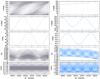 |
Fig. 11 Time evolution of the osculating orbital elements over a time span − 11 000 to + 1000 days from the epoch T0 = 2 456 224.724705, covered by observations of ξ Tau. Left: the semi-major axis a1, eccentricity e1, inclination i1, longitude of ascending node Ω1, and the argument of pericentre ω1 (poorly defined because e1 → 0) of the inner, eclipsing binary orbit (components Aa and Ab). Right: the same parameters a2,e2,i2,Ω2,ω2 for orbit 2 (i.e. components (Aa+Ab) and B). All these plots correspond to the simulation with χ2 = 2578, presented in Fig. 9. Variations in the inclination i1 and argument of pericentre ω2 are of major interest, since they result in observable effects. On the other hand, the distant orbit 3 (not shown here) exhibits only minor variations of its elements. The bump in the osculation elements of orbit 2 at JD ≈ 2 455 500 is related to the passage of component C through its pericentre. |
8.3. Differences between traditional and N-body models
Most importantly, orbital elements do change in the course of time; especially i1,Ω1,ω1,Ω2,ω2 seem to be critical in the case of ξ Tau (see Fig. 11). While the precession of ω2 was accounted for, the remaining terms were not. The precession of nodes Ω1, Ω2 about the total angular momentum axis occurs with a ≈ 19 yr period. In the Laplace plane, which is perpendicular to the total angular momentum, this would cause a circulation of Ω’s from 0° to 360°, but we can only see an oscillation of at most 3.5° that is due to the purely geometrical projection to the plane of the sky. There are also inevitable coupled oscillations of inclinations, with i1 ranging from 84.5° to 88.2°. All these rather expected secular effects are discussed in much more detail in Sect. 9.1.
Additionally, there are short-period oscillations not described by the secular theory. While a1 and a2 only oscillate about constant mean values, there seems to be a mid-term evolution of both e1 and e2, with amplitudes reaching 0.008, which is larger than the uncertainty of their initial values, that is,  . In this particular case, this is related to the periastron passage of component C.
We emphasise that it is absolutely necessary to use an N-body model (like ours), otherwise traditional methods assuming constant orbital elements (or precessing ωs only) may result in systematic discrepancies or artefacts. When the parameters reported in Table 15 are compared to those derived by classical models (Table 12), the general agreement between the elements is evident, but their uncertainty intervals do not always overlap. This is probably to be expected because we compare osculating (apples) and fixed orbital elements (oranges).
An outstanding example of how classical methods may fail is a detailed analysis of MOST light curves and the corresponding minima timings from 2012. At first, we thought that the uneven spacing of minima indicates a non-zero eccentricity of the inner orbit, e1 ≃ 0.002. However, this is in stark contrast with past RV measurements, which constrain forcing of e1(t) due to perturbations by component B and require e1(t = T0) → 0. Figure 12 shows upon close scrutiny that the oscillation of the semi-major axis a1 has a period 3.76 days, which is half of the synodic period Psyn1 of orbit 1, in a system that corotates with orbit 2. Moreover, its amplitude slightly decreases as component B moves farther away. These tiny perturbations are the real cause of the observed eclipse timing variations. They also allow us to discard mirror models with  and prefer those with Ω1 ≃ Ω2 because the resulting
  vs. 150 is significantly different. Again, the eclipse variations are explained in more detail in Sect. 9.2.
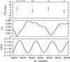 |
Fig. 12 Comparison of the osculating semi-major axis a1 (bottom) and eccentricity e1 evolution (middle) as computed by our N-body model for two mirror solutions with Ω1 ≃ 331° (bold solid) and |

8.4. Model with closure phases to resolve mirror solutions
The admissible solutions presented in Table 15 are degenerate in the sense that we cannot distinguish among several mirror models (in particular  ). To resolve this degeneracy, we constructed an N-body model that accounts for interferometric visibilities and closure phases. The latter are especially suitable to detect any asymmetries, while the former are necessary to correctly obtain (symmetric) angular positions and separations.
In addition to Eqs. (14) to (18), we have a few more relations:  (21)
(21) (22)
(22) (23)
(23) (24)
(24) (25)with the notation described in Table 16. The complex visibilities V′ and their triple products
  were computed assuming uniform disks for individual components. Relative luminosities Lij at a given effective wavelength λ were computed by a black-body approximation.
Notation used for additional coordinates and quantities needed in our extended N-body model.
This extended model minimises  and has nine additional free parameters: distance d to ξ Tau , uniform-disk radii Rj, and effective temperatures Teffj of all the components, even though the contribution of component C is only minor (clearly lower than 10% at the longest wavelength, λ = 2.6 μm).
We used all observational data from the MARKIII, NPOI, CHARA/VEGA, and VLTI/AMBER spectro-interferometers, with Nvis = 17 391 measurements of the squared visibility | V | 2 and Nclo = 4856 measurements of the closure phase argT3 (from NPOI and VLTI/AMBER). The total number of degrees of freedom is thus ν = Ndata−Mfree = 28 019−32 = 27 987. At the same time, we did not use astrometric positions ( ) of component B because they are not independent; all the information should be contained in | V | 2 and argT3 measurements.
Initially, we used nominal uncertainties and weights wvis = 1, wclo = 1, but the resulting  value was too high (≈ 105), even for our best-fit models (cf. Fig. 13). The most likely reason is that we did not account properly for all calibration uncertainties. To resolve this problem, an internal re-calibration would be necessary. A possible explanation for the too high χ2 has been given in Sect. 6. For example, CHARA/VEGA interferometry from Sept. 29 2012 exhibits unrealistically quick changes of | V | 2 at an almost constant baseline B/λ ≃ 1.3 to 1.4 × 10⁸ cycles (see Fig. C.8). In our case, we decreased the weight wvis = 0.1 to avoid it dominating other χ2 contributions (e.g. eclipse timing variations).
We focused on a limited set of seven mirror models, always with one or two modified orbital elements (see Table 17). For each of them, we performed one simplex run, verified by simulated annealing with the initial temperature 100 000 kelvin, schedule Ti + 1 = 0.99Ti and 100 iterations at given Ti, so that other free parameters were able to adapt themselves to a new situation, and we computed χ2s that are reported in the same table. If the final value remains relatively high, it means the model is not compatible with the respective interferometric data.
Clearly, we are sufficiently sensitive to resolve Ω2 and i2, that is, the longitude of the ascending node and the inclination of component B (see Fig. 14), but not directly to resolve Ω1, i1, or i3 elements. Consequently, we can discard  ,
,  and prefer Ω2 ≃ 331°, i2 ≃ 86° solution on the basis of the closure phase measurements alone.
Moreover, because our N-body model is constantly constrained by RV, ETV, ETD, and astrometric data, which prevent a convergence to unrealistic values of all the parameters, we can spot (in Table 17) that the squared visibility measurements are not compatible with  and
and  , therefore they were discarded as well and the Ω1 ≃ 329°, i1 ≃ 86° solution was preferred.
Finally, as demonstrated in Sect. 8.3, the N-body dynamics and ETV measurements allow us to safely discard any Ω1 ≠ Ω2, therefore we clearly prefer Ω1 = 329°. The only remaining ambiguity is thus the inclination i3 vs.  . To conclude this section, a combination of approximately orthogonal measurements (RV, ETV, ETD, | V | 2, argT3) leads to interesting and solid results, which is as expected.
We also comment on the fact that even this type of model may be insufficient. Other physical effects exist that we did not account for, such as tidal interactions of non-spherical stars, spin–orbital coupling, various magneto-hydrodynamic phenomena, or pulsations of (all) components. Their importance for the dynamics of ξ Tau is yet to be assessed.
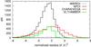 |
Fig. 13 Distributions of normalised residuals ( |


Summary of  and
and  values for squared visibility | V | 2 and closure phase argT3 measurements.
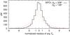 |
Fig. 14 Distributions of normalised residuals |


9. Dynamical evolution of the Aa+Ab+B subsystem
The osculating orbital elements shown in Fig. 11 exhibit many variations over different timescales, from the short period of the inner eclipsing binary, to the intermediate period of the orbital motion of component B with respect to the eclipsing binary, up to long periods of tens to hundreds of years. Are we able to understand some of these terms, including their amplitude, and determine parametric dependencies on stellar masses and periods of orbits 1 and 2? To do so, we need to turn to perturbation theory. In this section we neglect dynamical effects of the distant component C and focus on the triple subsystem Aa+Ab+B.
The hierarchy of the ξ Tau system implies a preferential choice of Jacobi coordinates to describe its dynamics, in which on the one hand, r is the relative position of Ab with respect to Aa, and on the other, R is the relative position of component B with respect to the barycentre of orbit 1. The conjugate momenta involve reduced masses  and
and  of orbits 1 and 2, with M1 = mAa + mAb and M2 = M1 + mB. To zero-order approximation, both systems evolve on Keplerian orbits, but their interaction introduces a perturbation that causes r and R to follow trajectories described by numerical integrations in Sect. 8 that are more complicated than Keplerian orbits. The elliptical approximation may be only applicable to a certain interval of time. The latter becomes short especially for compact systems. ξ Tau is a good representative of this class.
In the world of perturbation theory, both orbits 1 and 2 are represented by a set of osculating orbital elements that evolve in time as a result of their mutual interaction. From a plethora of perturbations described in this way, we recall two results relevant for the observed features of the ξ Tau system. We first describe the secular effects, whose duration is conveniently short for this compact system to be detected, and then some of the long- and short-period eclipse time variations in the eclipsing binary.
9.1. Secular effects
We define Delaunay momenta 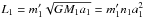 and
and 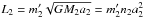 of orbits 1 and 2 (e.g. Harrington 1968, 1969; Soderhjelm 1975; Breiter & Vokrouhlický 2015). Here n1 and n2 are the mean motion values of the orbits 1 and 2, both related to the semi-major axes a1 and a2 through the third Kepler law:
  and
and  (G is the gravitational constant). In a secular approximation, when the orbital longitude for both orbits 1 and 2 is removed from the interaction (e.g. Harrington 1969; Breiter & Vokrouhlický 2015), the semi-major axes a1 and a2 are constant.
The dynamics of the Aa+Ab+B system may in principle be studied in an arbitrary reference frame. However, its description becomes very simple in a preferred frame that is often called Laplacian. The z-axis of this frame is aligned with the total orbital angular momentum of the system. To distinguish osculating orbital elements in the observer-oriented frame we used above, we denote the elements in the Laplacian frame with a tilde. For instance, the orbital inclinations for orbits 1 and 2 are denoted  and
and  , and the corresponding longitudes of nodes
  and
and  .
.
The secular evolution of the triple system is particularly simple when three conditions are met: the eccentricity e1 of the inner orbit is negligible, the mutual angle  , of orbital planes 1 and 2 is small, and the system is wide enough, such that on the timescale of interest only the quadrupole interaction of the inner and outer orbits is relevant. The mutual angle
  can be determined by the orbital elements in the observer reference frame using
  (26)These conditions fortunately currently apply to the ξ Tau system. We also note for the third condition that the octupole interaction is very small because of nearly equal masses in orbit 1, i.e., mAa ≃ mAb. The next secular contribution would arise from the non-linear quadrupole effect (e.g. Breiter & Vokrouhlický 2015), which is small on a timescale of some decades. Then, e1 = 0 is a stable solution, and e2 and are constant in time. When the orbital elements are referred to the invariable plane that is normal to the total angular momentum, the orbital inclinations and of orbits 1 and 2 are constant as well, and both orbital planes uniformly precess in the inertial space about the total angular momentum direction. Their nodes
  and
and  linearly advance with a rate (e.g. Soderhjelm 1975; Breiter & Vokrouhlický 2015)
 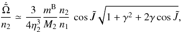 (27)where γ = L1/ (L2η2) is the ratio of the angular momenta of the two orbits, and
  . In triple systems the outer orbit typically has a dominant share of the total angular momentum of the system, thus γ< 1. For ξ Tau we have approximately γ ≃ 0.132. Unless precisely coplanar, the main effect of the orbital-plane precession is in periodic changes of inclinations i1 and i2 in the observer system. These variations directly affect magnitude depths of the eclipses, or might eventually cause the system to become non-eclipsing for a certain period of time.
In addition to the steady precession of the orbital planes, the second secular effect in the given setup consists of precession of the pericentre of the outer orbit. Denoting its longitude  , we have
 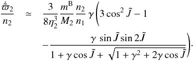 (28)Comparing Eqs. (27) and (28), we note that the pericentre precession frequency of the outer orbit is slower by a factor ≃ γ than the nodal frequency (assuming sufficiently small). Thus nodes and inclinations vary on shorter timescales than the argument of pericentre of orbit 2.
9.2. Long- and short-period eclipse variations
The mutual interaction of the orbits also results in a palette of periodic perturbations. So far, the long-period effects, namely those with a period P2 of orbit 2, have been extensively studied (e.g. Soderhjelm 1975, 1982; Borkovits et al. 2003, 2011, 2015). We here focus on the ETVs, that is, on advances and delays δtLP in epochs of eclipse of orbit 1 that are due to the variations in its mean motion n1 caused by component B. Assuming for simplicity coplanar orbits  deg, we obtain (e.g. Soderhjelm 1975; Borkovits et al. 2011, 2015; Rappaport et al. 2013, which also contain terms proportional to
  )
) 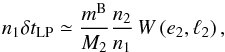 (29)with
  (30)where f2 and ℓ2 are the true and mean anomalies of orbit 2. For a low eccentricity e2 we have W ≃ 3e2sinℓ2. Obviously, the principal component of ETV in Eq. (29) becomes zero for a circular orbit 2 because it is related to variations of n1 triggered by variations in the distance R to component B.
In the course of this work, we noted that dominant short-period effects may also be of interest (those with the period of the inner orbit 1), provided high-quality eclipse data are collected. Using methods of first-order perturbation theory, we found that the leading short-period term reads 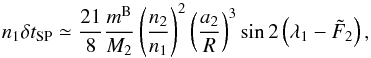 (31)where R is the distance of component B to the barycentre of the inner binary system, and
  is its true orbital longitude. The term has a period equal to half the synodic period of the Aa+Ab system in a reference frame corotating with the motion of component B.
This effect is not primarily dependent of the eccentricity e2 because it is triggered by variations in the mutual positions of components Aa and Ab with respect to component B. Its magnitude is smaller by a factor 0.4 at periastron and by 0.1 at apoastron of orbit 2. Nevertheless, the effect is not entirely negligible, and we found that it contributes to the observed eclipse shift in the MOST data (see Fig. 12).
9.3. Comparison of the secular theory with the results of the analytic and numerical models
Here we compare the apsidal motion detected with both analytic and numerical methods and additional secular and periodical variations of orbital elements predicted by the numerical model presented in Sect. 8
-
The apsidal motion of orbit 2: first, we useresults of the analytic theory above. Using nominal or-bital parameters from Table 12, we obtain
 deg, and consequently
  deg yr-1. We note that
  may be directly obtained from Eq. (28) because the nodal longitude Ω2 in the observer frame oscillates without any secular drift. This is about a third lower than the value detected with the analytic RV curve model (see Table 5), but in excellent agreement with the N-body model, whose prediction is
  deg yr-1, and with fit of the interferometric observations (see Table 11).
 -
The nodal motion of orbits 1 and 2: inserting nominal parameters from Table 12 provides the mean nodal drift
 deg yr-1 (Eq. (27)), which is again in excellent agreement with results of the N-body model; we note that the periods of the nodal oscillations are effectively ≃ 19.43 deg yr-1 for orbit of component A (Ω1) and ≃ 19.81 deg yr-1 for orbit B (Ω2). Values are not exactly the same, probably because of interaction with component C, which was not included in the perturbation theory. There is a hint of a shallower depth of the Hvar photometric observations from early 2007 when our model predicts a higher value of the inclination i1. However, to determine the inclination variations, we need more accurate photometric observations in the future.
 -
Eclipse-timing variations – orbit 1: Eqs. (29)–(31) provide amplitudes of the ETVs (assuming that component B is at periastron) of orbit 1 δtETV,long = 0.0162 ± 0.0007 d, δtETV,short = 0.0068 ± 0.0003 d. Their sum agrees with the detected amplitude of ETVs (δtETV,OBS = 0.025 ± 0.010 d). We also note that the two primary eclipse minima in the MOST data were found to be phase-shifted by ≃ 0.0003 in Sect. 4.3. This is about 0.1° in orbital longitude of inner orbit 1. Combining results in Eqs. (29)–(31) and taking into account ℓ2 ≃ 86° and λ1 ≃ F2 from Table 15, we obtain very good agreement with the observed shift.
10. Motivations for future observations of ξ Tauri
First, it seems desirable to continue the observations of the times of minima and, more importantly, eclipse duration and depth. At an epoch after approximately RJD 59 405.0, that is, in the second half of 2021, we would expect either persisting or disappearing eclipses of the inner pair Aa+Ab for different mirror solutions. Consequently, this is a direct and independent test of our analysis of closure phase measurements in Sect. 8.4. We note that the nominal solution shown in Fig. 11 exhibits too small variations of i1, such that the eclipsing binary would be eclipsing constantly.
Nevertheless, even the nominal solution predicts nearly 4° full amplitude of variation in i1 and we expect fairly well observable effects. We suggest, for instance, a space-born observation of a similar quality to that of MOST, obtained at the turn of 2016 and 2017, when the predicted i1 value would be highest (about 88.2°). The change in eclipse depth, as compared to the MOST data, should be about 0.05 mag, which is very easily detectable. Such a single observation would further constrain parameters of ξ Tau with an exceptional accuracy.
It would be of great help if the line spectra of the faint component C, separated by 200 to 600 mas from the triple Aa+Ab+B, were obtained and the corresponding RV measured. This would also allow us to distinguish between the remaining two mirror orbital solutions for the motion of this component.
Precise and uninterrupted space-based photometry on a longer time-span would be useful to unambiguously resolve oscillation modes and splittings. Given the high rotation frequency frot = 2.38 d-1 ≃ 27.5 μHz, it should not be that difficult (the minimum time-span Δt ≃ 1 /frot), but currently aliases with instrumental frequencies seem to limit the S/N in the Fourier spectrum.
As an alternative, series of high-resolution high S/N spectra would be needed to detect the oscillation modes independently, as the travelling sub-features in the line profiles of component B are broadened by a relatively high rotation. Precise RV measurements of components Aa and Ab may also reveal the Rossiter-McLaughlin effect, which gives the rotational sense of the two components.
A new series of long-baseline optical spectro-interferometric observations including measurements of closure phase are highly desirable, because they would provide a fully independent estimate of the orbital elements of orbit 1, would independently determine the sense of revolution of the components of orbit 1 with respect to orbit 2, and would finally provide an independent estimate of the radii of components Aa and Ab.
11. Conclusion
We have conducted an in-depth study of the quadruple stellar system ξ Tau, starting from simple analytic models for different types of observations (see Sects. 3−7), and concluding with a complex N-body model that combines astrometric, photometric, spectroscopic, and spectro-interferometric observations to a certain degree (see Sect. 8). We were able to set tight constraints on three components of ξ Tau, and they will provide an excellent test case for models of stellar evolution, while the full description of the geometry of the hierarchy will provide a test of the binary formation.
The analytic models allowed us to estimate properties of components Aa, Ab, and B that are highly consistent (see the critical summary of the analytic models in Sect. 7) and mean orbital elements of orbits 1, 2, and 3 using different methods that are again consistent with each other, but provided limited-to-no insight into the dynamic evolution of orbits of the ξ Tau.
This discrepancy was fixed with the N-body model, which properly accounts for the dynamic interaction within the system and is able to fit RVs, ETVs, and astrometric positions simultaneously. It provided a set of osculating elements and component masses whose evolution fits the observables (see Table 13). It also provided insight into the long- and short-term evolution of the osculating elements (see Fig. 11) and also resolved the prograde and retrograde solution (between orbits 1 and 2) solely from ETVs. The result also supports previous analyses because it did not vary much from their outcome.
Perturbation theory shows that the most pronounced secular evolution of elements, that is, the advance of the apsidal line of orbit 2, the harmonic variation of the inclination i1,2, and the longitude of the ascending node Ω1,2, are explained by a quadrupole interaction between orbits 1 and 2. The same applies to the predicted size of ETVs, which agree well with observations.
A detailed description with a simple tutorial how to use it is provided at https://github.com/chrysante87/pyterpol/wiki
![\hbox{$T_{\rm eff}^{\rm B} \in \left[13\,000, 14\,500\right]$}](/articles/aa/full_html/2016/10/aa28860-16/aa28860-16-eq713.png)
![\hbox{$T_{\rm eff}^{\rm Aa} \in \left[9000, 11\,500\right]$}](/articles/aa/full_html/2016/10/aa28860-16/aa28860-16-eq714.png)
![\hbox{$T_{\rm eff}^{\rm Ab} \in \left[9000, 11\,500\right]$}](/articles/aa/full_html/2016/10/aa28860-16/aa28860-16-eq715.png)
![\hbox{$L_{\rm R}^{\rm B} \in \left[0.55, 0.8\right]$}](/articles/aa/full_html/2016/10/aa28860-16/aa28860-16-eq722.png)
![\hbox{$L_{\rm R}^{\rm Aa} \in \left[0.10, 0.25\right]$}](/articles/aa/full_html/2016/10/aa28860-16/aa28860-16-eq723.png)
![\hbox{$L_{\rm R}^{\rm Ab} \in \left[0.10, 0.25\right]$}](/articles/aa/full_html/2016/10/aa28860-16/aa28860-16-eq724.png)
The program and a short user guide are available at http://astro.troja.mff.cuni.cz/ftp/hec/HEC27
LITpro software available at http://www.jmmc.fr/litpro
![\hbox{$\dot{\omega}_2\in\left[1.5, 4.0\right]$}](/articles/aa/full_html/2016/10/aa28860-16/aa28860-16-eq734.png)
The program used for these computations, including sources and all input data, is available at http://sirrah.troja.mff.cuni.cz/~mira/xitau/
The ranges expressed in Cartesian coordinates were zAb ∈ (−0.148,−0.088) au, zB ∈ (−1.47,−0.87) au, zC ∈ (−8.72,−2.72) au, vxAb ∈ (−0.092,−0.032) au d-1, vyAb ∈ (0.050,0.110) au d-1, vxB ∈ (−0.078,−0.018) au d-1, vyB ∈ (0.042,0.102) au d-1, vzB ∈ (−0.022,0.038) au d-1, vxC ∈ (−0.082,−0.022) au d-1, vyC ∈ (0.025,0.085) au d-1, and vzC ∈ (−0.030,0.030) au d-1.
Maxim DL is a commercial software designed for astronomical imaging, http://www.cyanogen.com/maxim/main.php
Visual Spec is a freeware designed for the wavelength calibration and the instrumental response removal, http://www.astrosurf.com/vdesnoux/index.html
The whole package along with a detailed manual, auxiliary data files, and results is available at http://astro.troja.mff.cuni.cz/ftp/PHOT
The user’s manual for the tool amdlib was developed at the Jean-Marie Mariotti Center and is publicly available at http://www.jmmc.fr/doc/index.php?search=JMMC-MAN-2720-0001
Acknowledgments
The research of J.N., P.H., M.W., and P.Z. was supported by grants P209/10/0715 and GA15-02112S of the Czech Science Foundation. The research of J.N. and P.H. was also supported by grant No. 678212 of the Grant Agency of the Charles University. The Navy Prototype Optical Interferometer is a joint project of the Naval Research Laboratory and the US Naval Observatory, in cooperation with Lowell Observatory and is funded by the Office of Naval Research and the Oceanographer of the Navy. The authors thank Jim Benson and the NPOI observational support staff, whose efforts made this project possible. This research has made use of the SIMBAD astronomical literature database, operated at CDS, Strasbourg, France. The CHARA Array is operated with support from the National Science Foundation through grant AST-0908253, the W. M. Keck Foundation, the NASA Exoplanet Science Institute, and from Georgia State University. This publication is supported as a project of the Nordrhein-Westfälische Akademie der Wissenschaften und der Künste in the framework of the academy programme by the Federal Republic of Germany and the state Nordrhein-Westfalen. H.B. acknowledges financial support by Croatian Science Foundation under the project 6212 “Solar and Stellar Variability”. The project is based on data obtained from the ESO Science Archive Facility under request number jnemravova217453, on spectral data retrieved from the ELODIE archive at Observatoire de Haute-Provence (OHP), and on observations made at the South African Astronomical Observatory (SAAO). PZ wish to thank the staff at SAAO for their warm hospitality and help with the equipment. A.F.J.M. is grateful for financial assistance to NSERC (Canada) and FQRNT (Quebec). The observations with the MPG 2.2 m telescope were supported by the Czech Ministry of Education, Youth and Sports project LG14013 (“Tycho Brahe: Supporting Ground-based Astronomical Observations”) during run P2 in May 2015. We acknowledge the use of the electronic database from the CDS, Strasbourg and electronic bibliography maintained by the NASA/ADS system. We acknowledge the constructive criticism by the referee Peter P. Eggleton, which helped us to improve the paper.
References
- Aller, L. H., Appenzeller, I., Baschek, B., et al. 1982, Landolt-Börnstein: Numerical Data and Functional Relationships in Science and Technology – New Series, Group 6 Astronomy and Astrophysics, Vol. 2 [Google Scholar]
- Armstrong, J. T., Mozurkewich, D., Rickard, L. J., et al. 1998, ApJ, 496, 550 [NASA ADS] [CrossRef] [Google Scholar]
- Baranne, A., Queloz, D., Mayor, M., et al. 1996, A&AS, 119, 373 [NASA ADS] [CrossRef] [EDP Sciences] [Google Scholar]
- Bolton, C. T., & Grunhut, J. H. 2007, in IAU Symp. 240, eds. W. I. Hartkopf, P. Harmanec, & E. F. Guinan, 66 [Google Scholar]
- Bonneau, D., Clausse, J.-M., Delfosse, X., et al. 2006, A&A, 456, 789 [NASA ADS] [CrossRef] [EDP Sciences] [Google Scholar]
- Borkovits, T., Érdi, B., Forgács-Dajka, E., & Kovács, T. 2003, A&A, 398, 1091 [NASA ADS] [CrossRef] [EDP Sciences] [Google Scholar]
- Borkovits, T., Csizmadia, S., Forgács-Dajka, E., & Hegedüs, T. 2011, A&A, 528, A53 [NASA ADS] [CrossRef] [EDP Sciences] [Google Scholar]
- Borkovits, T., Rappaport, S., Hajdu, T., & Sztakovics, J. 2015, MNRAS, 448, 946 [NASA ADS] [CrossRef] [Google Scholar]
- Breiter, S., & Vokrouhlický, D. 2015, MNRAS, 449, 1691 [NASA ADS] [CrossRef] [Google Scholar]
- Brož, M., Mayer, P., Pribulla, T., et al. 2010, AJ, 139, 2258 [NASA ADS] [CrossRef] [Google Scholar]
- Butterworth, S. 1930, Wireless Engineer, 7 [Google Scholar]
- Campbell, W. W. 1909, ApJ, 29, 224 [NASA ADS] [CrossRef] [Google Scholar]
- Claret, A. 1998, A&AS, 131, 395 [NASA ADS] [CrossRef] [EDP Sciences] [Google Scholar]
- Claret, A. 2001, MNRAS, 327, 989 [NASA ADS] [CrossRef] [Google Scholar]
- Degroote, P., Acke, B., Samadi, R., et al. 2011, A&A, 536, A82 [NASA ADS] [CrossRef] [EDP Sciences] [Google Scholar]
- de Laverny, P., Recio-Blanco, A., Worley, C. C., & Plez, B. 2012, A&A, 544, A126 [NASA ADS] [CrossRef] [EDP Sciences] [Google Scholar]
- Drimmel, R., Cabrera-Lavers, A., & López-Corredoira, M. 2003, A&A, 409, 205 [NASA ADS] [CrossRef] [EDP Sciences] [Google Scholar]
- Eggleton, P. P., & Kiseleva-Eggleton, L. 2001, ApJ, 562, 1012 [NASA ADS] [CrossRef] [Google Scholar]
- Eggleton, P. P., & Tokovinin, A. A. 2008, MNRAS, 389, 869 [NASA ADS] [CrossRef] [Google Scholar]
- ESA 1997, VizieR Online Data Catalog, I/239 [Google Scholar]
- Fabrycky, D., & Tremaine, S. 2007, ApJ, 669, 1298 [NASA ADS] [CrossRef] [Google Scholar]
- Fekel, J. F. C. 1981, ApJ, 246, 879 [NASA ADS] [CrossRef] [Google Scholar]
- Flower, P. J. 1996, ApJ, 469, 355 [NASA ADS] [CrossRef] [Google Scholar]
- Fuhrmann, K., Chini, R., Hoffmeister, V. H., et al. 2011, MNRAS, 411, 2311 [NASA ADS] [CrossRef] [Google Scholar]
- Glindemann, A., Albertsen, M., Andolfato, L., et al. 2004, in New Frontiers in Stellar Interferometry, ed. W. A. Traub, Proc. SPIE, 5491, 447 [Google Scholar]
- Hadrava, P. 1995, A&AS, 114, 393 [NASA ADS] [Google Scholar]
- Hadrava, P. 1997, A&AS, 122, 581 [NASA ADS] [CrossRef] [EDP Sciences] [Google Scholar]
- Hadrava, P. 2009, ArXiv e-prints [arXiv:0909.0172] [Google Scholar]
- Harmanec, P. 1988, Bulletin of the Astronomical Institutes of Czechoslovakia, 39, 329 [Google Scholar]
- Harmanec, P. 1998, A&A, 335, 173 [NASA ADS] [Google Scholar]
- Harmanec, P., & Horn, J. 1998, J. Astron. Data, 4, 5 [Google Scholar]
- Harmanec, P., Horn, J., & Juza, K. 1994, A&AS, 104, 121 [NASA ADS] [Google Scholar]
- Harrington, R. S. 1968, AJ, 73, 190 [NASA ADS] [CrossRef] [Google Scholar]
- Harrington, R. S. 1969, Celest. Mech., 1, 200 [Google Scholar]
- Hummel, C. A., Mozurkewich, D., Armstrong, J. T., et al. 1998, AJ, 116, 2536 [NASA ADS] [CrossRef] [Google Scholar]
- Hummel, C. A., Benson, J. A., Hutter, D. J., et al. 2003, AJ, 125, 2630 [NASA ADS] [CrossRef] [Google Scholar]
- Hummel, C. A., Zavala, R. T., & Sanborn, J. 2013, Central European Astrophysical Bulletin, 37, 127 [NASA ADS] [Google Scholar]
- Husser, T.-O., Wende-von Berg, S., Dreizler, S., et al. 2013, A&A, 553, A6 [NASA ADS] [CrossRef] [EDP Sciences] [Google Scholar]
- Kaufer, A., Stahl, O., Tubbesing, S., et al. 1999, The Messenger, 95, 8 [Google Scholar]
- Kraft, D. 1988, A software package for sequential quadratic programming, Deutsche Forschungs- und Versuchsanstalt für Luft- und Raumfahrt Köln: Forschungsbericht (Wiss. Berichtswesen d. DFVLR) [Google Scholar]
- Lafrasse, S., Mella, G., Bonneau, D., et al. 2010, VizieR Online Data Catalog, II/300 [Google Scholar]
- Lenz, P., & Breger, M. 2004, in The A-Star Puzzle, eds. J. Zverko, J. Ziznovsky, S. J. Adelman, & W. W. Weiss, IAU Symp., 224, 786 [Google Scholar]
- Levison, H. F., & Duncan, M. J. 2013, Astrophysics Source Code Library [record ascl:1303.001] [Google Scholar]
- Mason, B. D., Martin, C., Hartkopf, W. I., et al. 1999, AJ, 117, 1890 [NASA ADS] [CrossRef] [Google Scholar]
- Moultaka, J., Ilovaisky, S. A., Prugniel, P., & Soubiran, C. 2004, PASP, 116, 693 [NASA ADS] [CrossRef] [Google Scholar]
- Mourard, D., Clausse, J. M., Marcotto, A., et al. 2009, A&A, 508, 1073 [NASA ADS] [CrossRef] [EDP Sciences] [Google Scholar]
- Mozurkewich, D., Armstrong, J. T., Hindsley, R. B., et al. 2003, AJ, 126, 2502 [NASA ADS] [CrossRef] [Google Scholar]
- Nemravová, J. A., Harmanec, P., Bencheikh, J., et al. 2013, Central European Astrophysical Bulletin, 37, 207 [NASA ADS] [Google Scholar]
- Palacios, A., Gebran, M., Josselin, E., et al. 2010, A&A, 516, A13 [NASA ADS] [CrossRef] [EDP Sciences] [Google Scholar]
- Petrov, R. G., Malbet, F., Weigelt, G., et al. 2007, A&A, 464, 1 [NASA ADS] [CrossRef] [EDP Sciences] [Google Scholar]
- Press, W. H., Teukolsky, S. A., Vetterling, W. T., & Flannery, B. P. 1993, Numerical Recipes in FORTRAN: The Art of Scientific Computing, 2nd edn. (New York: Cambridge University Press) [Google Scholar]
- Prša, A., & Zwitter, T. 2005, ApJ, 628, 426 [NASA ADS] [CrossRef] [Google Scholar]
- Prša, A., & Zwitter, T. 2006, Ap&SS, 304, 347 [NASA ADS] [CrossRef] [Google Scholar]
- Rappaport, S., Deck, K., Levine, A., et al. 2013, ApJ, 768, 33 [NASA ADS] [CrossRef] [Google Scholar]
- Rica Romero, F. M. 2010, Rev. Mexicana Astron. Astrofis., 46, 263 [NASA ADS] [Google Scholar]
- Shao, M., Colavita, M. M., Hines, B. E., et al. 1988, A&A, 193, 357 [NASA ADS] [Google Scholar]
- Simon, K. P., & Sturm, E. 1994, A&A, 281, 286 [NASA ADS] [Google Scholar]
- Soderhjelm, S. 1975, A&A, 42, 229 [Google Scholar]
- Soderhjelm, S. 1982, A&A, 107, 54 [NASA ADS] [Google Scholar]
- Steiner, I., Stahl, O., Seifert, W., Chini, R., & Quirrenbach, A. 2008, in SPIE Conf. Ser., 7014, 4 [Google Scholar]
- Stellingwerf, R. F. 1978, ApJ, 224, 953 [NASA ADS] [CrossRef] [Google Scholar]
- Storn, R., & Price, K. 1997, Journal of Global Optimization, 11, 341 [CrossRef] [Google Scholar]
- Tallon-Bosc, I., Tallon, M., Thiébaut, E., et al. 2008, in SPIE Conf. Ser., 7013, 70131J [Google Scholar]
- ten Brummelaar, T. A., McAlister, H. A., Ridgway, S. T., et al. 2005, ApJ, 628, 453 [NASA ADS] [CrossRef] [Google Scholar]
- Tody, D. 1986, in Instrumentation in astronomy VI, ed. D. L. Crawford, SPIE Conf. Ser., 627, 733 [Google Scholar]
- Tody, D. 1993, in Astronomical Data Analysis Software and Systems II, eds. R. J. Hanisch, R. J. V. Brissenden, & J. Barnes, ASP Conf. Ser., 52, 173 [Google Scholar]
- Tokovinin, A. A. 1997, A&AS, 124, 75 [NASA ADS] [CrossRef] [EDP Sciences] [Google Scholar]
- Tokovinin, A., Mason, B. D., Hartkopf, W. I., Mendez, R. A., & Horch, E. P. 2015, AJ, 150, 50 [NASA ADS] [CrossRef] [Google Scholar]
- van Belle, G. T., Creech-Eakman, M. J., & Hart, A. 2009, MNRAS, 394, 1925 [NASA ADS] [CrossRef] [Google Scholar]
- van Leeuwen, F. 2007, A&A, 474, 653 [NASA ADS] [CrossRef] [EDP Sciences] [Google Scholar]
- Walker, G., Matthews, J., Kuschnig, R., et al. 2003, PASP, 115, 1023 [NASA ADS] [CrossRef] [Google Scholar]
- Zasche, P., & Wolf, M. 2007, Astron. Nachr., 328, 928 [NASA ADS] [CrossRef] [Google Scholar]
- Zasche, P., Uhlář, R., Kučáková, H., Svoboda, P., & Mašek, M. 2014, IBVS, 6114, 1 [NASA ADS] [Google Scholar]
Appendix A: Supplementary material to the spectroscopic observations and their analyses
Details of the reduction procedure of the spectroscopic observations used in this study along with supplementary material to its analysis are given in this section.
Appendix A.1: Acquisition and reduction of the spectroscopic observations
The reduction procedure applied to spectra from different observatories (the labelling of observatories corresponds to that introduced in Table 2) were the following:
-
1.
OND: all slit spectra were secured at the coudé focus of the 2 m reflector in Ondřejov, Czech Republic, and were recorded with the CCD detector PyLoN 2048x512BX. The bias subtraction, flat-fielding, and wavelength calibration were carried out using IRAF9 (Tody 1986, 1993). The spectra were normalised with Hermite polynomials (order k ≤ 10).
-
2.
FER: the echelle spectra were acquired with the 2.2 m ESO/MPG reflector at La Silla, Chile, and were reduced (bias subtraction, flat-fielding, and wavelength calibration) with a MIDAS pipeline developed specifically for the instrument (Kaufer et al. 1999). The studied regions of the reduced spectra were normalised with Hermite polynomials (order k ≤ 10).
-
3.
BES: the spectra were acquired with an echelle spectrograph mounted at the 1.5 m Hexapod Telescope at Cerro Amazones, Chile, which is the same as the FEROS spectrograph, and the same MIDAS pipeline was used to carry out the reduction (bias subtraction, flat-fielding, wavelength calibration). The studied regions were normalised with Hermite polynomials (order k ≤ 10).
-
4.
ELO: the echelle spectra were obtained with the 1.93 m reflector at Observatory Haute-Provence. The initial reductions (bias subtraction, flat-fielding, wavelength calibration) were carried out with a pipeline described in Baranne et al. (1996). The studied regions were normalised with Hermite polynomials (order k ≤ 10).
-
5.
DDO: the slit spectra were acquired with the 1.88 m reflector at the David Dunlap Observatory. The initial reductions (bias subtraction, flat-fielding, wavelength calibration) were carried out using IRAF. The spectra were normalised with Hermite polynomials (order k ≤ 10).
-
6.
LIS: the slit spectra were acquired with the 0.356 m reflector at the Astronomical Observatory of the Instituto Geográfico do Exército, Lisbon. The dark-frame subtraction and flat-fielding were carried out in Maxim DL10. The wavelength calibration was carried out using neon comparison spectra and telluric lines in the program Visual Spec11. The instrumental response was also removed in this program, using Castor as a reference star. The spectra were normalised with Hermite polynomials (order k ≤ 10).
Appendix A.2: Supplementary materials to the analysis of spectroscopic observations
The spectroscopic supplementary material consists of Fig. A.1 that shows a comparison of the separated and synthetic profiles. The related analyses are described in Sects. 3.5 and 3.3.
 |
Fig. A.1 Comparison of the separated and synthetic spectra. The parameters defining the synthetic spectra are listed in Table 6. In each panel we show in the top spectrum component B, in the middle spectrum component Aa, and in the bottom spectrum component Ab. The thick grey line plots spectra, the thin black line separated and re-normalised spectra, and the thin red line synthetic spectra. The residuals are computed for synthetic and re-normalised separated spectra. |
Appendix B: Supplementary material to the photometric observations and their analysis
Details on the reduction procedure of the photometric observations used in this study along with supplementary material to their analysis are given in this section.
Appendix B.1: Acquisition and reduction of the photometric observations
The reduction procedure applied to photometric observations from different observatories (the labelling of observatories corresponds to the labelling introduced in Table 3) were the following:
-
1.
HVAR: the differential observations were obtained with the 0.65 m reflector at the Hvar Observatory, Croatia, which is equipped with a photoelectric photometer with an EMI 6256 tube. The observations were acquired relative to the comparison star 4 Tau with the check star 6 Tau observed as frequently as ξ Tau and transformed to the standard UBV system (UBVR for observations acquired after RJD = 56 000) using the non-linear transformations implemented in the reduction package HEC2212 (see Harmanec et al. 1994; Harmanec & Horn 1998). All observations were reduced with the latest release 18, which allows for time variation in the linear extinction coefficients in the course of the observing night.
-
2.
HIPP: the all-sky observations were acquired with the 0.29 m reflector of the Hipparcos satellite and transformed to V magnitude using the formulae derived by Harmanec (1998).
-
3.
SAAO: the differential observations were acquired at the South African Astronomical Observatory, South Africa with 0.5 m reflector equipped with a photoelectric photometer. The observations were acquired relative to the comparison star 4 Tau and 6 Tau served as a check star and were transformed to the standard Johnson system using HEC22.
-
4.
VILL: the differential observations were acquired with the Automatic Photometric Telescope at Villanova, USA. The observations were taken relative to the comparison star 4 Tau and 6 Tau served as a check star.
-
5.
MOST: the all-sky observations were obtained with the 0.15 m reflector in the MOST satellite. The initial reduction was carried out according to Walker et al. (2003) and references therein. Removal of the remaining instrumental artefacts and the stray light from Earth’s atmosphere is described in Sect. 2.
Appendix B.2: Supplementary materials to the analysis of the photometric observations
The photometric supplementary material consists of Figs. B.1 and B.2 that show the available primary and secondary light-curve minima. All minima cover a time interval no longer than 30 d. See Sect. 4 for related analyses.
 |
Fig. B.1 All available primary minima of orbit 1. The filters are denoted as follows: UBV – Johnson UBV filters, MO the MOST filter, and A differential measurements taken in the visible without any filter. Mean RJD is given in the bottom left corner of each panel. |
 |
Fig. B.2 All available secondary minima of orbit 1. The filters are denoted as follows: UBV – Johnson UBV filters, MO the MOST filter, A differential measurements taken in the visible without any filter. Mean RJD is given in the bottom left corner of each panel. |
Appendix C: Supplementary material to the spectro-interferometric observations and their analyses
Details on the acquisition and reduction of the spectro-interferometric observations, along with tables and figures illustrating their analysis are presented here.
Appendix C.1: Mark III observations
The observations were carried out using a single north-south baseline three times on January 19, October 19, and November 2, 1991. The baseline length was 32 m on the first night and 15 m on the two other nights. Visibilities were recorded in three narrow-band channels at 5000 Å, 5500 Å, and 8000 Å. μ and η Tau (limb-darkened diameters of 0.41 mas and 0.98 mas, respectively, with 10% uncertainties) served as the calibrators. The calibrated visibilities were obtained from the Mark III data archive, which was created using the reduction and calibration methods described by Mozurkewich et al. (2003).
Appendix C.2: NPOI observations
The observations were carried out with the three-beam combiner in 1998 and 2000, and from 2003 to 2013 with the six-beam combiner. Visibilities, complex triple amplitudes, and closure phases were recorded in 16 narrow-band channels between 5500 Å and 8500 Å. The journal of the NPOI observations including the calibrator stars is given in Table C.2, and the calibrator information is given in Table C.4.
The calibrators were taken from a list of single stars maintained at NPOI with diameters estimated from V and (V−K) using the surface brightness relation by Mozurkewich et al. (2003) and van Belle et al. (2009). Values of E(B−V) were derived from comparison of the observed and theoretical colours as a function of spectral type by Schmidt-Kaler in Aller et al. (1982). Values for the extinction derived from E(B−V) were compared to estimates based on the maps by Drimmel et al. (2003), and used to correct V if they agreed within 0m.5. Even though the surface brightness relation based on (V−K) colours is to first order independent of the reddening, we included this small correction. The minimum (squared) visibility amplitudes corresponding to the diameter estimates are given in Table C.4 for all NPOI observations and show that the calibrators are either unresolved or only weakly resolved.
NPOI data and their reductions were described by Hummel et al. (1998) and Hummel et al. (2003). For the first time, we used a pipeline written in GDL13 for the OYSTER14 NPOI data reduction package. The pipeline automatically edits the one-second averages produced by another pipeline directly from the raw frames, based on expected performance such as the variance of fringe tracker delay, photon count rates, and narrow-angle tracker offsets. Visibility bias corrections are derived as usual from the data recorded away from the stellar fringe packet. After averaging the data over the full length of an observation, the closure phases of the calibrators were automatically unwrapped so that their variation with time, as well as that of the visibility amplitude, could be interpolated for the observations of ξ Tau. For the calibration of the visibilities, the pipeline used all calibrator stars observed during a night to obtain smooth averages of the amplitude and phase-transfer functions using a Gaussian kernel of 80 min in length. The residual scatter of the calibrator visibilities and phases around the average set the level of the calibration uncertainty and was added in quadrature to the intrinsic data errors. The amplitude calibration error of typically a few percent in the red channels up to 15% in the blue channels was added in quadrature to the intrinsic error of the visibilities. The phase calibration was good to about a couple of degrees.
Appendix C.3: VEGA/CHARA observations
The observations were carried out during two runs in 2011 and in 2012. Preliminary results, based on the observations obtained during the first run, were published by Nemravová et al. (2013). The reduction procedure was the same for both runs.
Five observations were acquired in 2011. All observations were obtained in the three-telescope (3T) mode and included the CHARA baselines E1E2W2, W1W2S2, and W2E2S2, ranging from 63 m to 245 m (E1, E2, S1, S2, W1, and W2 denote the telescopes in the CHARA telescope array). Ten new observations were secured in 2012. Four of them were taken in the 3T mode and the remaining six were taken in the two-telescope (2T) mode. The 2T observations included the CHARA baselines S2S1 and E2E1, their projected lengths ranging from 34 m to 66 m. The 3T observations contained the E2E1W2 and W2W1S1 baselines, their projected lengths were from 65 m to 279 m. A detailed journal of all interferometric observations with the instrument CHARA/VEGA is in Table C.3.
The observations were obtained with two cameras centred on 5350 Å (denoted BLUE) and 7300 Å (denoted RED) at spectral resolution R ≃ 5000. Individual frames were recorded with a frequency of 100 Hz and grouped into blocks containing 2500 frames. Each block was coherently summed and each observation had from 20 to 90 blocks. Two 20 nm wide bands were chosen in the BLUE region and two 30 nm wide bands in the RED region. The four bands used are ΔλIF = { 5320−5520,5400−5600,7000−7300,7300−7600 }15 Å. The frames were summed within these bands and the raw squared visibility VRAW was derived from the sum. The spectral bands have to be narrow because of the limited coherence of the waves due to the atmospheric turbulence. There are no strong stellar lines in any of the four spectral bands used; the spectral band 7300−7600 Å is affected by the telluric water vapour lines, but even those are smeared out by the low resolution of the spectra.
A calibrator was observed before and after each observation of ξ Tau. Calibrators were selected with the tool SearchCal (Bonneau et al. 2006), and their list along with their basic properties is given in Table C.5. The instrumental visibility was estimated according to the formulae  (C.1)where
  is the calibrated visibility of ξ Tau,
  the raw visibility of ξ Tau,
  the visibility of a uniform disk with a diameter listed in Table C.5, and
  the raw visibility of a calibrator. To avoid inaccurate observations, we removed all blocks with a S/N< 2 and whose optical path delay (OPD) differed from the mean OPD by more than 2σ. Such blocks usually represent only random noise rather than a physical signal. In rare cases, when the raw visibility of ξ Tau was close to zero, but safely detected, and there was no suitable observation of a calibrator, the raw visibilities of ξ Tau were used in the analysis as if they were calibrated, but they were assigned an error ΔV2 = 0.05. This allowed us to save more usable observations for very long baselines giving strong constraints by low-visibility measurements.
Appendix C.4: VLTI/AMBER observations
ξ Tau was observed by VLTI/AMBER in 2012 Dec. 03. The observations were acquired in three-telescope mode in J, H, and K bands and the low-resolution regime (R = 35). The baselines ranged from 41 m to 139 m.
The unprocessed observations were downloaded from the ESO archive and the reduction was made with the AMBER data reduction software amdlib16. Following the manual step by step, we applied the bad pixel and flat-field maps, computed pixel-to-visibility matrix, subtracted the dark frame, and performed frame selection based on the fringe S/N ratio (the best 20% were kept).
Four stars were used as calibrators; they are listed along with their basic properties is in Table C.5. The uniform-disk diameters were taken from the JMMC Stellar Diameters Catalogue (Lafrasse et al. 2010). The calibration was made using the library amdlib.
Additionally, we had to filter the data. Observations with an effective wavelength at the edges of the J, H, and K bands were not removed, although they had large uncertainties and displayed an abrupt drop in visibility inconsistent with the remaining data. Only observations whose effective wavelength lay in any of following bands Δλ ∈ { 1.155−1.34;1.49−1.77;2.02−2.05;2.075−2.41 }μm were used. Furthermore, several observations suddenly had very low visibility compared to neighbouring data, which was very likely caused by an instrumental and/or atmospheric effect. These are data taken at RJD = 56 264.767145, all data with B/λ< 1.76 × 10⁷, and data taken from RJD = 56 264.776653 to RJD = 56 264.778568 with B/λ> 9.25 × 10⁷.
Appendix C.5: Night-by-night analysis of NPOI observations
The calibrated visibility and phase estimates are rich enough to permit night-by-night estimation of positions of individual components. Owing to the lower resolution, the NPOI interferometer is almost insensitive to orbit 1 and diameters of the three components (Aa, Ab and B) of ξ Tau. Therefore the system was represented by two point sources, and the relative position of component B and the eclipsing binary was estimated. The results of the night-by-night analysis are given in Table C.1.
The uncertainty ellipses of position of the photocentre of orbit 1 (which is almost identical with its centre of mass because the two components of the eclipsing binary are similar) relative to component B were computed from fits to contours of the χ2 surfaces at the minima instead of deriving them from the interferometric PSF to take the limitations of fitting a component position very far from the phase centre into account. For the contour we chose 25% above minimum to obtain a reduced .
An astrometric fit to positions listed in Table C.1 confirms that NPOI is insensitive to the eclipsing binary because the derived orbital properties do not differ significantly from those obtained from a global fit to V2 presented in Table 11.
Astrometric positions of the photocentre of orbit 1 relative to component B derived from night-by-night analysis of MARK III and NPOI observations.
Appendix C.6: Supplementary materials to the analysis of the spectro-interferometric observations
The spectro-interferometric supplementary material consists of the following tables and figures:
-
1.
Table C.2 lists all available spectro-interferometric observations acquired with the NPOI and MARK III instruments. For each observation the observing stations, its baselines [Bmin;Bmax], phase coverage of orbits 1, and 2 φ1, and, φ2, and associated calibrators are given. The numbering of calibrators is given in Table C.4.
-
2.
Table C.3 lists all available spectro-interferometric observations acquired with the CHARA/VEGA instrument. For each observation the lengths of the projected baselines B and their orientation θ, the phase coverage of orbits 1, and 2 φ1, and, φ2, and associated calibrators are given.
-
3.
Table C.4 lists all calibrators which were used to calibrate the NPOI observations of ξ Tau. For each calibrator its Johnson V magnitude, spectral type, colour index V−K, interstellar reddening E(B−V), the minimum amplitude squared visibility V2, and the uniform disk diameter θV−K for wavelength range from V to K band are given.
-
4.
Table C.5 lists all calibrators which were used for calibration of the CHARA/VEGA and VLTI/AMBER observations. For each calibrator the spectral type, effective temperature Teff, gravitational acceleration log g, Johnson V (K) magnitude V (K), and the uniform disk diameter in these bands θV, θK are given.
-
5.
Figures C.1–C.10 show fits of the global model given by Eq. (9), and corresponding parameters are listed in Table 11.
NPOI and MARK III observations of ξ Tau.
Journal of CHARA/VEGA spectro-interferometric observations of ξ Tau.
List of NPOI calibrators used for ξ Tau.
List of stars used for calibration of CHARA/VEGA and VLTI/AMBER observations.
 |
Fig. C.1 Best-fitting model (part one) plotted against the observations from the MARKIII and NPOI spectro-interferometers. In each panel, the observed squared visibility V2 is plotted with red triangles; the model corresponding to parameters listed in Table 11 is denoted with black points. Residuals of the fit are shown below each panel. The mean acquisition date, the corresponding mean heliocentric Julian date, and the instrument are indicated above each panel. |
 |
Fig. C.2 Best-fitting model (part two) plotted against the observations from the NPOI spectro-interferometer. In each panel, the observed squared visibility V2 is plotted with red triangles; the model corresponding to parameters listed in Table 11 is denoted with black points. Residuals of the fit are shown below each panel. The mean acquisition date, the corresponding mean reduced heliocentric Julian date, and the instrument are indicated above each panel. |
 |
Fig. C.3 Best-fitting model (part three) plotted against the observations from the NPOI spectro-interferometer. In each panel, the observed squared visibility V2 is plotted with red triangles; the model corresponding to parameters listed in Table 11 is denoted with black points. Residuals of the fit are shown below each panel. The mean acquisition date, the corresponding mean reduced heliocentric Julian date, and the instrument are indicated above each panel. |
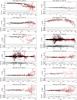 |
Fig. C.4 Best-fitting model (part four) plotted against the observations from the NPOI spectro-interferometer. In each panel, the observed closure phase T3φ is plotted with red triangles; the model corresponding to parameters listed in Table 11 is denoted with black points. Residuals of the fit are shown bellow each panel. The mean acquisition date, the corresponding mean reduced heliocentric Julian date, and the instrument are indicated above each panel. |
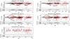 |
Fig. C.5 Best-fitting model (part five) plotted against the observations from the NPOI spectro-interferometer. In each panel, the observed closure phase T3φ is plotted with red triangles; the model corresponding to parameters listed in Table 11 is denoted with black points. Residuals of the fit are shown bellow each panel. The mean acquisition date, the corresponding mean reduced heliocentric Julian date, and the instrument are indicated above each panel. |
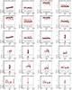 |
Fig. C.6 Best-fitting model (part six) plotted against the observations from the CHARA/VEGA spectro-interferometer. In each panel, the observed squared visibility V2 is plotted with red triangles; the model corresponding to parameters listed in Table 11 is denoted with black points. Residuals of the fit are shown below each panel. The mean acquisition date, the corresponding mean reduced heliocentric Julian date, and the instrument are indicated above each panel. |
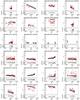 |
Fig. C.7 Best-fitting model (part seven) plotted against the observations from the CHARA/VEGA spectro-interferometer. In each panel, the observed squared visibility V2 is plotted with red triangles; the model corresponding to parameters listed in Table 11 is denoted with black points. Residuals of the fit are shown below each panel. The mean acquisition date, the corresponding mean reduced heliocentric Julian date, and the instrument are indicated above each panel. |
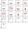 |
Fig. C.8 Best-fitting model (part eight) plotted against the observations from the CHARA/VEGA spectro-interferometer. In each panel, the observed squared visibility V2 is plotted with red triangles; the model corresponding to parameters listed in Table 11 is denoted with black points. Residuals of the fit are shown below each panel. The mean acquisition date, the corresponding mean reduced heliocentric Julian date, and the instrument are indicated above each panel. |
 |
Fig. C.9 Best-fitting model (part nine) plotted against the observations from the VLTI/AMBER spectro-interferometer. In each panel, the observed squared visibility V2 is plotted with red triangles; the model corresponding to parameters listed in Table 11 is denoted with black points. Residuals of the fit are shown below each panel. The mean acquisition date, the corresponding mean reduced heliocentric Julian date, and the instrument are indicated above each panel. |
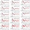 |
Fig. C.10 Best-fitting model (part ten) plotted against the observations from the VLTI/AMBER spectro-interferometer. In each panel, the observed closure phase T3φ is plotted with red triangles; the model corresponding to parameters listed in Table 11 is denoted with black points. Residuals of the fit are shown bellow each panel. The mean acquisition date, the corresponding mean reduced heliocentric Julian date, and the instrument are indicated above each panel. |
Appendix D: Description of the observational material
This section contains templates of tables with observational material. The full tables are available at the CDS.
-
Radial velocity measurements are published inTable D.1.
-
Photometric observations are published separately for each photometric filter (MO, U, B, V) in Tables D.2–D.5.
-
The spectro-interferometric observations are published in form of calibrated squared visibility moduli in Table D.6, and closure phases in Table D.7.
Reduced photometric observations acquired with the MOST satellite.
Reduced photometric observations acquired in the Johnson U filter.
Reduced photometric observations acquired in the Johnson B filter.
Reduced photometric observations acquired in the Johnson V filter.
Calibrated squared visibility moduli estimated from studied spectro-interferometric observations.
Closure phases estimated from studied spectro-interferometric observations.
All Tables
Orbital elements obtained by KOREL(spectral disentangling) for all available spectra containing at least one of the studied regions.
Parameters of the best-fitting circular orbital model obtained with the program PHOEBE 1.0.
Orbital elements of orbit 3 based on a fit to astrometric measurements published in WDS.
Summary of parameters derived from the spectroscopic, photometric, and spectro-interferometric analyses.
Notation used for various coordinates, velocities, and uncertainties that we used in our N-body model.
Initial osculating orbital elements aj,ej,ij,Ωj,ωj,Mj of the ξ Tau system as derived by our N-body model.
Notation used for additional coordinates and quantities needed in our extended N-body model.
Summary of and values for squared visibility | V | 2 and closure phase argT3 measurements.
Astrometric positions of the photocentre of orbit 1 relative to component B derived from night-by-night analysis of MARK III and NPOI observations.
Calibrated squared visibility moduli estimated from studied spectro-interferometric observations.
All Figures
|
Fig. 1 Coverage of orbits 1 and 2 with the spectro-interferometric observations. The outer plot: the black line denotes the orbit of the centre of mass of the eclipsing binary relative to component B (which resides at the beginning of the coordinate system of the outer plot), and red dots denote the relative position of the centre of mass of the eclipsing binary relative to component B at the epochs of spectro-interferometric observations. The inset plot: the black line denotes the orbit of component Ab relative to component Aa (which resides at the beginning of the coordinate system of the inset plot), and red dots denote the relative position of component Ab relative to component Aa at epochs of spectro-interferometric observations. In both plots the orbital elements are invariable, i.e. they do not show the true orbits 1 and 2 as they would appear on the sky, but only demonstrate that the spectro-interferometric observations sample the orbits well enough to constrain elements of both orbits. |
| In the text | |
|
Fig. 2 RVs of the centre of gravity of the eclipsing binary (red triangles) and component B (blue triangles) against the best-fitting model (black) corresponding to parameters listed in Table 5. ΔAa,Ab (in km s-1) denote residuals of the fit for RVs of the centre of gravity of the eclipsing binary, and ΔB (in km s-1) residuals of the fit for RVs of component B. |
| In the text | |
|
Fig. 3 RVs of components Aa (red) and Ab (blue) relative to the centre of gravity of the eclipsing binary against the best-fitting model (black) listed in Table 5. ΔAa,Ab are residuals of the fit for components Aa and Ab. |
| In the text | |
|
Fig. 4 Example of the fit of the synthetic spectra (red) to three observed spectra (black) in spectral regions: 1) Δλ1 = [4280,4495] Å (top), 2) Δλ2 = [4815,4940] Å (middle), 3) Δλ3 = [6330,6390] Å (bottom, left), 4) Δλ3 = [6660,6695] Å (bottom, right). The synthetic spectra are given by parameters listed in Table 7. |
| In the text | |
|
Fig. 5 Fit of the light curve from the satellite MOST. Only the light curve minima and their surroundings are shown. The primary (secondary) minimum is on the left (right) on each panel. The left panel corresponds to the global circular solution e1 = 0.0 and to orbital period P1 = 7.14664 d. The right panel corresponds to a local solution, where small adjustment of the eccentricity and the orbital period was allowed. MO denotes the satellite broad-band filter. |
| In the text | |
|
Fig. 6 Fourier spectrum of the MOST light curve from Fig. 7 (i.e. outside eclipses). Prominent frequency peaks are marked (see their description in Sect. 4.1). |
| In the text | |
|
Fig. 7 Normalised light curve as reduced from MOST photometry, but without intervals of primary and secondary eclipses (top panel), together with the corresponding period P0 (middle) and amplitude A0 (bottom) of the harmonic function f(t) = 1 + C0 + A0sin [ 2π(t−T0) /P0 + φ0 ], which was sequentially fitted to the light curve, always in limited intervals ΔE1 = 0.5 of the epoch (indicated by the black double arrow), shifted with a step ΔE2 = 0.05. The oscillations exhibit both frequency and amplitude modulations, with periods spanning P0 = (0.42 ± 0.01) d and amplitudes A0 = (0.00060 ± 0.00015) mag. It seems that the longest P0 and the largest A0 are observed at around primary eclipses and vice versa. |
| In the text | |
|
Fig. 8 Speckle-interferometric outer orbit 3 corresponding to the solution of Table 10. The dotted line stands for the line of apsides, the dashed line for the line of nodes. |
| In the text | |
|
Fig. 9 One of the best-fit solutions for the ξ Tau system with our N-body model and using all available observational data. In this case, the resulting total χ2 is 2578, while the number of degrees of freedom ν = 908. Top: radial velocities vzbAa, vzbAb, vzbB, vzbC of the individual components; model values are denoted by lines (component Aa is black, not clearly visible, Ab grey, B blue, and C orange), observations by black error bars and residuals by thick red lines. Middle: O−C values for both primary and secondary minima timings; model timings are denoted by black points (very densely packed), observations by grey crosses, and O−C with its uncertainty by red error bars. Bottom left: astrometric positions of component B based on NPOI interferometric observations; model orbit xpB, ypB with respect to photocentre Aa+Ab (i.e. not w.r.t. B, as usually) is again denoted by a blue line, observations by black error bars and residuals by thick red lines. The orbit is not a single ellipse, but rather a complex trajectory that quickly precesses and is moreover affected by (slight) photocentre motions. Bottom right: similarly, astrometric positions of the distant component C xpC, ypC with respect to the Aa+Ab+B photocentre is denoted by an orange line. Component B is relatively luminous, which makes the orbit in these photocentric coordinates slightly jagged. |
| In the text | |
|
Fig. 10 Example of the one-dimensional χ2 mapping used to derive uncertainties of orbital elements for the ξ Tau system. The dependencies of the χ2 values on the three nodes Ω1, Ω2, Ω3 are shown, while the remaining elements correspond to the best-fit values from Table 15. The preferred solution for Ω1 ≃ 331°, with χ2 = 2578, and a hint of a mirror solution at Ω1 ≃ 151° are clearly visible. If the latter is optimised separately, we would obtain χ2 as low as 2 749. The sudden increase of |
| In the text | |
|
Fig. 11 Time evolution of the osculating orbital elements over a time span − 11 000 to + 1000 days from the epoch T0 = 2 456 224.724705, covered by observations of ξ Tau. Left: the semi-major axis a1, eccentricity e1, inclination i1, longitude of ascending node Ω1, and the argument of pericentre ω1 (poorly defined because e1 → 0) of the inner, eclipsing binary orbit (components Aa and Ab). Right: the same parameters a2,e2,i2,Ω2,ω2 for orbit 2 (i.e. components (Aa+Ab) and B). All these plots correspond to the simulation with χ2 = 2578, presented in Fig. 9. Variations in the inclination i1 and argument of pericentre ω2 are of major interest, since they result in observable effects. On the other hand, the distant orbit 3 (not shown here) exhibits only minor variations of its elements. The bump in the osculation elements of orbit 2 at JD ≈ 2 455 500 is related to the passage of component C through its pericentre. |
| In the text | |
|
Fig. 12 Comparison of the osculating semi-major axis a1 (bottom) and eccentricity e1 evolution (middle) as computed by our N-body model for two mirror solutions with Ω1 ≃ 331° (bold solid) and |
| In the text | |
|
Fig. 13 Distributions of normalised residuals ( |
| In the text | |
|
Fig. 14 Distributions of normalised residuals |
| In the text | |
|
Fig. A.1 Comparison of the separated and synthetic spectra. The parameters defining the synthetic spectra are listed in Table 6. In each panel we show in the top spectrum component B, in the middle spectrum component Aa, and in the bottom spectrum component Ab. The thick grey line plots spectra, the thin black line separated and re-normalised spectra, and the thin red line synthetic spectra. The residuals are computed for synthetic and re-normalised separated spectra. |
| In the text | |
|
Fig. B.1 All available primary minima of orbit 1. The filters are denoted as follows: UBV – Johnson UBV filters, MO the MOST filter, and A differential measurements taken in the visible without any filter. Mean RJD is given in the bottom left corner of each panel. |
| In the text | |
|
Fig. B.2 All available secondary minima of orbit 1. The filters are denoted as follows: UBV – Johnson UBV filters, MO the MOST filter, A differential measurements taken in the visible without any filter. Mean RJD is given in the bottom left corner of each panel. |
| In the text | |
|
Fig. C.1 Best-fitting model (part one) plotted against the observations from the MARKIII and NPOI spectro-interferometers. In each panel, the observed squared visibility V2 is plotted with red triangles; the model corresponding to parameters listed in Table 11 is denoted with black points. Residuals of the fit are shown below each panel. The mean acquisition date, the corresponding mean heliocentric Julian date, and the instrument are indicated above each panel. |
| In the text | |
|
Fig. C.2 Best-fitting model (part two) plotted against the observations from the NPOI spectro-interferometer. In each panel, the observed squared visibility V2 is plotted with red triangles; the model corresponding to parameters listed in Table 11 is denoted with black points. Residuals of the fit are shown below each panel. The mean acquisition date, the corresponding mean reduced heliocentric Julian date, and the instrument are indicated above each panel. |
| In the text | |
|
Fig. C.3 Best-fitting model (part three) plotted against the observations from the NPOI spectro-interferometer. In each panel, the observed squared visibility V2 is plotted with red triangles; the model corresponding to parameters listed in Table 11 is denoted with black points. Residuals of the fit are shown below each panel. The mean acquisition date, the corresponding mean reduced heliocentric Julian date, and the instrument are indicated above each panel. |
| In the text | |
|
Fig. C.4 Best-fitting model (part four) plotted against the observations from the NPOI spectro-interferometer. In each panel, the observed closure phase T3φ is plotted with red triangles; the model corresponding to parameters listed in Table 11 is denoted with black points. Residuals of the fit are shown bellow each panel. The mean acquisition date, the corresponding mean reduced heliocentric Julian date, and the instrument are indicated above each panel. |
| In the text | |
|
Fig. C.5 Best-fitting model (part five) plotted against the observations from the NPOI spectro-interferometer. In each panel, the observed closure phase T3φ is plotted with red triangles; the model corresponding to parameters listed in Table 11 is denoted with black points. Residuals of the fit are shown bellow each panel. The mean acquisition date, the corresponding mean reduced heliocentric Julian date, and the instrument are indicated above each panel. |
| In the text | |
|
Fig. C.6 Best-fitting model (part six) plotted against the observations from the CHARA/VEGA spectro-interferometer. In each panel, the observed squared visibility V2 is plotted with red triangles; the model corresponding to parameters listed in Table 11 is denoted with black points. Residuals of the fit are shown below each panel. The mean acquisition date, the corresponding mean reduced heliocentric Julian date, and the instrument are indicated above each panel. |
| In the text | |
|
Fig. C.7 Best-fitting model (part seven) plotted against the observations from the CHARA/VEGA spectro-interferometer. In each panel, the observed squared visibility V2 is plotted with red triangles; the model corresponding to parameters listed in Table 11 is denoted with black points. Residuals of the fit are shown below each panel. The mean acquisition date, the corresponding mean reduced heliocentric Julian date, and the instrument are indicated above each panel. |
| In the text | |
|
Fig. C.8 Best-fitting model (part eight) plotted against the observations from the CHARA/VEGA spectro-interferometer. In each panel, the observed squared visibility V2 is plotted with red triangles; the model corresponding to parameters listed in Table 11 is denoted with black points. Residuals of the fit are shown below each panel. The mean acquisition date, the corresponding mean reduced heliocentric Julian date, and the instrument are indicated above each panel. |
| In the text | |
|
Fig. C.9 Best-fitting model (part nine) plotted against the observations from the VLTI/AMBER spectro-interferometer. In each panel, the observed squared visibility V2 is plotted with red triangles; the model corresponding to parameters listed in Table 11 is denoted with black points. Residuals of the fit are shown below each panel. The mean acquisition date, the corresponding mean reduced heliocentric Julian date, and the instrument are indicated above each panel. |
| In the text | |
|
Fig. C.10 Best-fitting model (part ten) plotted against the observations from the VLTI/AMBER spectro-interferometer. In each panel, the observed closure phase T3φ is plotted with red triangles; the model corresponding to parameters listed in Table 11 is denoted with black points. Residuals of the fit are shown bellow each panel. The mean acquisition date, the corresponding mean reduced heliocentric Julian date, and the instrument are indicated above each panel. |
| In the text | |
Current usage metrics show cumulative count of Article Views (full-text article views including HTML views, PDF and ePub downloads, according to the available data) and Abstracts Views on Vision4Press platform.
Data correspond to usage on the plateform after 2015. The current usage metrics is available 48-96 hours after online publication and is updated daily on week days.
Initial download of the metrics may take a while.