| Issue |
A&A
Volume 593, September 2016
|
|
|---|---|---|
| Article Number | A6 | |
| Number of page(s) | 12 | |
| Section | Interstellar and circumstellar matter | |
| DOI | https://doi.org/10.1051/0004-6361/201628815 | |
| Published online | 29 August 2016 | |
Prestellar core modeling in the presence of a filament
The dense heart of L1689B
1 Université Grenoble
Alpes, IPAG, 38000 Grenoble, France
2 CNRS, IPAG, 38000
Grenoble,
France
3 Max-Planck-Institut für Astronomie,
Königstuhl 17,
69117
Heidelberg,
Germany
e-mail: This email address is being protected from spambots. You need JavaScript enabled to view it.
4 University Observatory Munich,
LMU Munich, Scheinerstr.
1, 81679
Munich,
Germany
Received:
28
April
2016
Accepted:
17
June
2016
Abstract
Context. Lacking a paradigm for the onset of star formation, it is important to derive basic physical properties of prestellar cores and filaments like density and temperature structures.
Aims. We aim to disentangle the spatial variation in density and temperature across the prestellar core L1689B, which is embedded in a filament. We want to determine the range of possible central densities and temperatures that are consistent with the continuum radiation data.
Methods. We apply a new synergetic radiative transfer method: the derived 1D density profiles are both consistent with a cut through the Herschel PACS/SPIRE and JCMT SCUBA-2 continuum maps of L1689B and with a derived local interstellar radiation field. Choosing an appropriate cut along the filament major axis, we minimize the impact of the filament emission on the modeling.
Results. For the bulk of the core (5000−20 000 au) an isothermal sphere model with a temperature of around 10 K provides the best fits. We show that the power law index of the density profile, as well as the constant temperature can be derived directly from the radial surface brightness profiles. For the inner region (<5000 au), we find a range of densities and temperatures that are consistent with the surface brightness profiles and the local interstellar radiation field. Based on our core models, we find that pixel-by-pixel single temperature spectral energy distribution fits are incapable of determining dense core properties.
Conclusions. We conclude that, to derive physical core properties, it is important to avoid azimuthally-averaging core and filament. Correspondingly, derived core masses are too high since they include some mass of the filament, and might introduce errors when determining core mass functions. The forward radiative transfer methods also avoids the loss of information owing to smearing of all maps to the coarsest spatial resolution. We find the central core region to be colder and denser than estimated in recent inverse radiative transfer modeling, possibly indicating the start of star formation in L1689B.
Key words: stars: formation / radiative transfer / submillimeter: ISM / ISM: clouds
© ESO, 2016
1. Introduction
For decades, no global answer has been known to the question of what ends the life of a prestellar low-mass core and starts the star formation process (Bergin & Tafalla 2007). Is it the weakening of a supporting force based on magnetic fields or turbulence, is it an internal or external kinetic trigger, or a mass overload? As recent data, e.g., from Herschel, better probe the complex filamentary network from which cores emerge, attention also turns to the role of the hosting filaments (André et al. 2014).
To find the physical reason of the star formation onset, substantial effort has been put in determining the basic properties of prestellar cores and filaments (Marsh et al. 2016), that is the gas density and temperature structures (Schmalzl et al. 2014) and the topology of the velocity field (Hacar & Tafalla 2011; Hacar et al. 2013).
Tracing the gas physical properties directly by the line emission of molecules is difficult since their abundances and excitation conditions vary with the physical properties so that different molecular emission lines trace different regions. Unfortunately, their abundances are also reduced by a freeze-out onto the dust grains because of the low temperatures around 10 K. Therefore, hardly any molecular tracers are available in the central region where the star formation process is initiated (Maret et al. 2013). Hence, the gases’ physical structure is determined from the radiation emitted or scattered by small dust grains that are mixed in the gas (e.g., Launhardt et al. 2013), and that also have the same temperature as the gas above a certain density threshold.
One of the “standard” prestellar cores that was investigated in detail both by analyzing its line emission and by dust radiative transfer (RT) effects is the core B68 (e.g., Alves et al. 2001). The most complete modeling of the core was performed by Nielbock et al. (2012) based on dedicated Herschel far-infrared (FIR) continuum maps and ancillary sub-mm continuum maps (we refer to this paper for a list of references for work on B68). A particularly interesting result of their ray-tracing analysis was the steep slope of the radial density profile (∝ r-3.5 azimuthally averaged for radii r> 60′′ with density deviations up to a factor of 4 in certain directions). Prestellar cores are expected to have density profiles resembling that of an isothermal sphere (Shu 1977) or of a Bonnor-Ebert sphere (BES; e.g., McLaughlin & Pudritz 1996), which are characterized by a decrease ∝ r-2 in the outer parts. Magnetized simple filament models have steeper gradients perpendicular to the filament axis ∝ r-4 (Ostriker 1964). However, for weak magnetization, Tilley & Pudritz (2003) found ∝ r-2. For the general problem of collapsing cylinders see also Hennebelle (2003). More recent theoretical work (e.g., Fischera & Martin 2012; Smith et al. 2014) suggests flatter profiles closer to an r-2-decline, in agreement with observational studies (e.g., Palmeirim et al. 2013). Because its environment and that of the neighboring cores only show weak remnants of the hosting filament, and its outer density profile is steeper than expected for a Bonnor-Ebert sphere model, B68 might not be representative of most prestellar cores. According to André et al. (2014), 70% of all cores identified in the Herschel Gould Belt Survey (HGBS) are located in a filament. Hence, it appears that the common mode of the onset of star formation may be a core that is still embedded and potentially affected by the hosting filament.
In this work, we therefore analyze the well-known core-filament system L1689B in the Ophiuchus star-forming region. The central part of the core shows depletion of gaseous molecules (e.g., CO, Jessop & Ward-Thompson 2001), but the level of depletion is moderate so that the core is either young, or has evolved quickly towards high degrees of concentration.
The core presents line asymmetries seen in e.g. CS(2−1), H2CO(212−111) and HCO+(3−2), which are commonly interpreted as indication of infall motions (Bacmann et al. 2000; Gregersen & Evans 2000; Lee et al. 2001). However, the projection along the line-of-sight and limited spatial resolution make the interpretation difficult. Additional velocity components have been proposed: L1689B may show oscillations as suggested for some cores by Lada et al. (2003) and Broderick & Keto (2010). Redman et al. (2004) argued that a rotating, non-infalling core center with a size of 3000 au may account for the shape of the line profiles seen in HCO+. Seo et al. (2013) considered the effect of internal velocities on the stability of BES. Analyzing L1689B, they concluded that the infall motion hints towards a kinematic disturbance as the motions are larger than expected for spontaneous gravitational infall.
Schnee et al. (2013) compared the degree of deuterium fractionation with infall velocities calculated from the HCO+ spectra. They find that the Jeans stability is a useful indicator of collapse. Calculating the Jeans mass, however, relies on the knowledge of the temperature and the outer core radius which seems to be unclear for L1689B: the derived masses and central column density of the core from the literature span a surprisingly wide range, with non-overlapping uncertainties. According to Kirk et al. (2005) and Makiwa et al. (2016) L1689B is a low-mass core with 0.4 ± 0.1 M⊙ and 0.49 ± 0.05 M⊙, respectively. Contrary, Bacmann et al. (2000) and Roy et al. (2014, R+14 hereafter) give a core mass of 11 M⊙ and 11 ± 2 M⊙, respectively, about a factor of 20 larger than in Kirk et al. (2005).
The central column densities for H2 were derived as 1.4 ± 0.1 × 1026 m-2, 3.6 ± 0.1 × 1026 m-2, and 5 × 1026 m-2 by Makiwa et al. (2016), R+14, and Kirk et al. (2005), respectively. Concerning the central temperature, the three publications give dust temperatures in the range 9.3−13 K (10.9 ± 0.2 K, 9.8 ± 0.5 K, and 11 ± 2 K, respectively). The distance estimates range from 120 pc (Loinard et al. 2008; Lombardi et al. 2008) over 140 pc (R+14) to 165 pc (Crapsi et al. 2005). In this work, we use 140 pc for the sake of comparison with R+14.
From these results, L1689B seems to be a core that already undergoes collapse although it is still chemically young. However, the rather low central densities derived in the aforementioned studies seem difficult to reconcile with the fact that the core is already collapsing. The density structure should show a strong central increase as it is seen for the core L1544 and expected for a contracting BES (Keto & Caselli 2010). Along this way, three difficulties arise.
- (1)
Is dust continuum modeling of single-dish telescope data ableto reveal a central density increase on length scales of a few1000 au (henceforth, we use the abbreviationkau = 1000 au)? R+14 haveapplied an Abel transform technique to L1689B (and B68)deriving density and dust temperature profiles from Herscheldust emission maps. It requires, however, tosmear the continuum maps at the different wavelengths to a single(coarse) resolution which decreases the sensitivity to centralgradients.
- (2)
How is the mass of the core determined when the core is located within a filament and a spherically or elliptically symmetric model mixes surface brightness contributions from core and filament in the maps?
- (3)
Because of the strong shielding of external radiation due to the steep density increase in the core center, the core temperature decreases towards the center. Is the decreased efficiency of dust thermal emission at low temperatures hindering the detection of the central density enhancements? Pagani et al. (2015) stressed this point concerning a potential reservoir of central cold dust (<8 K) that could be missed in the Herschel data modeling leading to errors in the derived total core mass. They argued that the ambiguity in dust mass estimates from FIR/mm data alone give rise to mass uncertainties to up to 70% for L1689B.
In this work, we address these three questions. We perform forward RT modeling of five FIR and submillimeter continuum maps of the core-filament system L1689B (Herschel PACS/SPIRE, JCMT/SCUBA-2) and additional RT modeling based on a grid of possible local radiation fields. In Sect. 2 we investigate physical motivations and practical criteria to distinguish core and filament also based on hydrodynamical calculations results obtained with the code RAMSES, and propose a scheme to extract the core emission from the total emission. The basic numerical method to derive the core density and temperature is discussed in Sect. 3 and applied in Sect. 4. This section also explains an additional method to remove ambiguities in the modeling by estimating the outer radiation field from the dust emission in all model shells. In Sect. 5, we compare our findings with earlier obtained results about the interstellar radiation field (ISRF), the mass and column density of L1689B, about determining dense core properties based on pixel-by-pixel single temperature spectral energy distribution (SED) fitting, the impact of filaments on the core mass function, the impact of opacity changes, and the mass of cold dust with temperatures <8 K in L1689B.
2. Disentangling core and filament
There are several motivations to distinguish the prestellar core and filament.
-
1.
Symmetry change in the spatial model: with a core showingcentral symmetry embedded in a filament with expected axialsymmetry, the break-down of the spherical symmetryassumption marks also a border for the applicability of1D models.
-
2.
Stability against gravitational collapse: the simplest way to evaluate the stability of the core is to determine the Jeans mass which requires to know the core radius that is not well-defined in a core-filament system.
-
3.
Region with gas contributing to the star formation process: not all of the core and filament gas will end in the star. Physically interesting is the region where gas and dust that are able to fall onto the central region before the star has reached its final mass. Its border is difficult to determine and likely more complex than estimating the free-fall radius for a given evolution time.
-
4.
Region with gas affecting the central temperature: since the central core temperature depends on the incoming radiation, the outer core and filament matter affects the physics in the star formation zone. The main consequence for low-mass cores is a shielding by outer regions. Also this border is difficult to find as usually the 3D geometry of the system is unknown and shielding effects strongly depend on 3D sight lines.
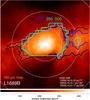 |
Fig. 1 Contours where the intensity of the core reaches the filament maximal intensity (reference point between the two vertical sub-filaments) for the different wavelengths. The color-coded image shows the 160 μm map. |
2.1. Core-filament border estimates
A first method to distinguish core and filament comes from looking at the maps where the intensity of the core has dropped to the mean maximal value of the filament outside the core. We used the L1689B Herschel PACS and SPIRE (Griffin et al. 2010) HGBS (André et al. 2010) data1. Figure 1 shows the 160 μm map where the filament is seen in most detail and overlaid contours where this value is reached. As reference points, we chose the point with the maximal filament intensity to the right of the core between the two vertical sub-filaments. This avoids confusion with the overlapping sub-filaments to the right but still characterizes the maximal intensity expected from the main filament. Comparing with the white circles at 10, 20, and 30 kau shows that this value is reached at radii between 8 kau and 15 kau depending on the location within the filament. We note that the limiting contour radius only weakly depends on the wavelengths. This means that the radiation we receive from radii of 20 kau or larger is clearly dominated by the filament.
More insight into distinguishing core and filament can be gained from a glance at typical results from hydrodynamical calculations of a core-forming filament system. Figure 2 shows a cut through an isothermal core-filament simulation H2 number density cube (Heigl et al. 2016) after about 1 Myr of filament evolution aiming to provide a simple model for the cores in L1517. The simulations were performed in 3D with the RAMSES code (Teyssier 2002). The cores form on the dominant fragmentation wavelength of a gravitational instable, infinite filament without magnetic fields. The resulting velocity structure of the core-forming motions is in excellent agreement with the observed velocities in L1517.
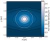 |
Fig. 2 Cut through the H2 number density structure including the core center for a hydro-dynamical simulation of the evolution of a filament with the RAMSES code. The white circle indicates the radius where the density deviation from spherical symmetry exceeds 50%. |
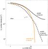 |
Fig. 3 Cuts through the H2 number density RAMSES results along the filament axis (thick black), with the maximal filament density subtracted (thick, dashed), and perpendicular to the filament axis (orange). The thin solid line indicates the steepness of a powerlaw with the exponent −1.73 which approximates the dashed line in a region around 10 kau. |
From the inner parts outwards, the core density structure evolves from spherical to elliptical symmetry. The white circle indicates the radius where the density deviation from spherical symmetry exceeds 50%. This radius is in this case about 4/5 of the filament width. As visible in Fig. 3, cuts starting in the core center perpendicular to the filament axis reach this value at about 10 kau (orange line). The thick black line gives the cut along the filament axis which reaches the maximal filament density value (thin dotted horizontal line) between 15 and 20 kau. Subtracting this value leads to the contribution of the core along the filament (dashed line). While the perpendicular cut intermixes the spatial gradients of core and filament, a horizontal cut is the line with the smallest gradients in the filament contribution, and by subtracting the filament maximal value gives the best measure of the core contribution. Indeed, subtracting the filament contribution, the simulation data show a radial power law in the outer core parts where disentangling core and filament is more difficult (dashed line). The exponent of the power law −1.73 is not far from the simple isothermal sphere value −2 (see thin line).
2.2. Choice of the cut in the plane-of-sky
With these findings in mind, we designed the modeling of the core located in the filament based on cuts through the Herschel maps along the filament axis. The basic approach is sketched in Fig. 4. We consider a plane that contains the filament axis and the line-of-sight and a core that is optically thin at all considered FIR/mm wavelengths. We assume that the radiative contribution of the filament along lines-of-sight behind and in front of the core can be approximated by the contribution by the filament outside the core. To determine the contribution of the core, the filament contribution is subtracted.
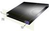 |
Fig. 4 Sketch of the horizontal cut along the filament main axis in the plane-of-sky. The cut has a height corresponding to the beam size at the considered wavelengths. The density in the plane of lines-of-sight is indicated in grey-scale along with the shells of the spherical density model. |
However, the core-filament system L1689B shows more complexity than this simple model. As visible in the surface representation of the map at λ = 160 μm (Fig. 5), the filament has sub-structure with smaller filaments running perpendicular to the main filament to the right of the core. Moreover, also the core center shows substructure but since this structure is not seen at longer wavelengths, we interpret it as a low density warmer sub-filament behind or in front of the core. Since there is less confusion from sub-structure to the East of the core, we start with modeling the cut from the center to the West and discuss other cuts in Sect. 2.4.
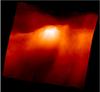 |
Fig. 5 Surface representation of the L1689B Herschel PACS map at 160 μm amplifying the substructure. The main filament axis is rotated horizontally and the core is in the center. Two narrow filaments are visible on the right perpendicular to the main filament, and the filament shows a narrow substructure along the main filament axis west of the core. There is also sub-structure visible in the central core region at this wavelength. |
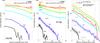 |
Fig. 6 Left and middle: radial cuts of the Herschel maps of L1689B in western direction from the core center. The numbers indicate the wavelength. Calibration error bars are added for the middle panel. The exponential shape of the 850 μm profile is better visible in the lin-log representation. The horizontal thin lines indicates the offset surface brightness from the filament. The two thin blue lines estimate the slope variation in the 800 μm-profile. Right: after subtracting the offsets, all profiles are close to an exponential function with approximately the same exponent A. The dotted lines show the exponential function with A = 0.11. The dashed vertical lines give the distance where deviations from the exponential occur. |
2.3. Filament removal unfolding a simple core structure
The left panel of Fig. 6 shows the resulting surface brightness profiles at the various wavelengths as a function of the distance in the western direction from the core center without any filament subtraction in log-log-representation. The Herschel profiles up to 500 μm merge into the almost constant filament surface brightness at large (>15 kau) distances. With the declining relative contribution to the surface brightness of the filament at longer wavelengths, more insight can come from submillimeter images. Therefore also cuts from the 850 μm SCUBA-2 and 1.3 mm map are included in our analysis. The SCUBA-2 data are part of the JCMT Gould Belt survey (Ward-Thompson et al. 2007), and are described in Pattle et al. (2015). The IRAM 30 m data are taken from Andre et al. (1996). These ground-based maps are not very sensitive to the filament’s emission, as observing techniques to remove atmospheric emission also filter out large spatial scales. Indeed, especially the 850 μm profiles show an exponential drop without a filament contribution at larger distances.
A clearer picture emerges when plotting the same data in log-lin-representation (middle panel of Fig. 6). The 850 μm profile which should mainly show the radiation from the core is well-represented by a straight declining line and therefore can be approximated by an exponential function. Following our modeling approach, we approximate the offset in surface brightness by the radiation from the filamentary dust behind and in front of the core by the surface brightness that we have measured in the filament near but outside the core (the approximately flat profile parts in the middle panel of Fig. 6 labeled “offsets”). We also added calibration error bars and two thin blue lines to estimate the slope range at 850 μm for the left figure.
The result of the subtraction is shown in the right plot of the same figure. We note that the data are shown only up to 25 kau in the left panel since according to Fig. 1 the contribution from the core becomes negligible for larger distances.
Interestingly, the surface brightness profiles at all wavelengths follow the same pattern and can be well fitted by a simple exponential function of the form ![Mathematical equation: \begin{equation} I(y)=I_0\ \exp\left[-\frac{Ay}{{\rm kau}}\right]\cdot \end{equation}](/articles/aa/full_html/2016/09/aa28815-16/aa28815-16-eq21.png) (1)The exponent shows little variation around A = 0.11 (dotted lines, with a variation of 0.1 to 0.12 read, e.g., from the middle panel for the 800 μm-profile) except for the 1.3 mm profile which is slightly steeper A = 0.16. As mentioned in Andre et al. (1996), the dual-beam observing technique used to map the core at 1.3 mm induces a filtering of the large spatial scales, which leads to an underestimation of the total flux as well as a steepening of the radial intensity profile. Hence, we did not further consider the 1.3 mm data to avoid introducing large errors from a misinterpretation of the surface brightness loss. This loss of flux at large spatial scales also affects the SCUBA-2 data but to a much smaller extent, since spatial scales up to 5′ can be recovered (Pattle et al. 2015), which is larger than the size of the core. The vertical dashed line indicates where deviation from the exponential shape occur.
(1)The exponent shows little variation around A = 0.11 (dotted lines, with a variation of 0.1 to 0.12 read, e.g., from the middle panel for the 800 μm-profile) except for the 1.3 mm profile which is slightly steeper A = 0.16. As mentioned in Andre et al. (1996), the dual-beam observing technique used to map the core at 1.3 mm induces a filtering of the large spatial scales, which leads to an underestimation of the total flux as well as a steepening of the radial intensity profile. Hence, we did not further consider the 1.3 mm data to avoid introducing large errors from a misinterpretation of the surface brightness loss. This loss of flux at large spatial scales also affects the SCUBA-2 data but to a much smaller extent, since spatial scales up to 5′ can be recovered (Pattle et al. 2015), which is larger than the size of the core. The vertical dashed line indicates where deviation from the exponential shape occur.
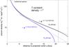 |
Fig. 7 Line-of-sight integral through an iso-thermal sphere (solid) can be approximated in large parts by an exponential (dotted). |
Exponential profiles are not unknown when it comes to integrating spherically symmetric density structures in order to obtain a column density profile. In Fig. 7 we show the column density profile of an isothermal sphere with a power law density profile ∝ r-2, and truncated at radius Rc (solid lines). Between the steep rise caused by the singularity at r = 0 and the cutoff at the core outer radius Rc the column density profile is well-described by exactly the same exponential shape that we observe in the L1689B surface brightness profiles (dotted lines). For more general density profiles with a power law of the form r− α, the factor A is numerically found to depend on the ratio α/Rc. For α = 2, A reaches 0.11 as observed for outer core radii of about Rc = 28 kau. We note that at this value the column density vanishes, but at shorter distances of about 21 kau for A = 0.11 deviations from the exponential become visible (dashed line). We therefore restrict modeling of the core up to 21 kau.
In the more realistic model of a Bonnor-Ebert sphere with a central flattening, the pole at y = 0 disappears and depending on the radial extent of the flattened region the agreement with the exponential function can extend to smaller distances.
We conclude that for radii >5 kau, the core shows approximately the same surface brightness distribution at all wavelengths once the filament contribution is removed following the simple scheme that we have described. The resulting surface brightness profiles already enable a direct interpretation without any radiative transfer modeling. They are consistent with radiation from an isothermal spherical core with a radial density profile following an r-2-dependence calculations. In the following we use the exponential approximation for the profiles with an outer radius of Rc = 28 kau between 5 kau and 21 kau. As visible from Fig. 6, the deviations of the observed surface brightness values from the exponential approximations are of the order of the calibration errors which enter the radiative transfer modeling performed in Sect. 4. We therefore consider that the impact of this approximation on the derived densities and temperatures is comparable to that caused by the calibration errors.
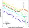 |
Fig. 8 Offset-subtracted surface brightness profiles for the Eastern cut along the filament axis (thick) in comparison to the Western cut (thin dashed, Fig. 6). The exponential fit leads to steeper gradients (A = 0.14) than for the Western cut. The surface brightnesses at 160 and 250 μm are enhanced due to a vertical filament in the region around 20 kau distance. |
2.4. Modeling for other cuts than the Western profile
The proposed method based on cuts along the filament axis can also be applied to the other direction (East). Figure 8 shows the resulting offset-subtracted surface brightness profiles for a cut in Eastern direction (thick line) for the various maps. For the sake of comparison we have added the Western cuts as thin dashed line. Again, the profiles reveal the same exponential shape for all wavelengths but with a slightly steeper gradient A = 0.14 than for the Western cut. It is more difficult to read the distance at which deviations from the exponential approximation occur due to the vertical filament that affects the map at distances of about 20 kau (visible in the 160 and 250 μm profiles). The only profile showing a clear decline is the 350 μm profile starting at about 19 kau. According to Fig. 7 this would correspond to a density gradient of about −2 again as for the Western cut. But due to the confusion with the sub-filament this conclusion is to be handled with caution.
It could also be considered to model a vertical cut. In a similar manner as the horizontal cuts, the filament off-core could be subtracted from a vertical central cut through the core to retrieve the core contribution. For a symmetric core filament system like the simple density structure seen in the RAMSES simulations (Fig. 2), this would lead to an approximate estimate of the core density. The L1689B filament, however, shows stronger asymmetries. Indeed, the filament profiles on both sides of the cores differ substantially as visible in Fig. 9. Vertical cuts through the 250 μm map divided into a Western, a central, and an Eastern box show a narrow maximum in the surface brightness to the West while the Eastern profiles are broader. In the central inlet, the white vertical profiles are compared to approximate fits of the left and right central profiles. In this case it is difficult to decide which profile would have to be subtracted to arrive at the core surface brightness profile.
Therefore, we rely in our analysis on the Western surface profiles noting that the Eastern profiles appear to have a similar underlying density structure.
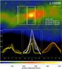 |
Fig. 9 Vertical surface brightness profiles (y direction) in the 250 μm map in three boxes left, central, and right around the core. The left box shows the narrow filament maximum (indicated again in the middle box as yellow line). The right box shows a broader maximum (at about the same level, see brown line in the middle box). The central cuts are shown as white lines in the middle box. Dotted circles indicate the distance from the center. |
3. Basic numerical method: peeling radiative transfer
Our calculations of the core density and temperature are adapted to the centrally-condensed structure of L1689B. The RT calculations are simple since L1689B is optically thin for the observed wavelengths discussed here (λ> 160 μm) which leads to a decoupling of the radiative contributions of all parts in the core-filament system (as already pointed out by R+14). For line transfer in core-filament systems we also refer to Smith et al. (2012) and for continuum transfer in filaments to Malinen 2012 Malinen et al. (2012). We use forward ray-tracing where the term forward is referring to first choosing a density and temperature and then determining the observed radiation. In this work, we only use a set of spherically symmetric shells but the used ray-tracing method described here works with any sort of centrally condensed layer structures and the cutpoints and segment lengths of the rays and layers are easy to determine even for complex layer structures. For the plane sketched in Fig. 4 the shells and rays are shown in Fig. 10. For simplicity we show rays for a cut in the Eastern direction while the cut through L1689B runs westward. We chose to describe the core with 18 concentric shells of 1 kau thickness, two outer shells of 5 kau thickness, all with constant density and temperature. (Fig. 8). The contribution to the emission of each shell at each radius can be easily calculated, starting from the outermost shell inwards (“peeling”). The density and temperature of shell i can be determined by single temperature SED fitting of the shell contribution to the overall intensity at radius i − 1. We investigated the impact of beam convolution comparing the un-convolved profiles with beam-convolved cuts with a 29 point stencil Gaussian beam pattern (Fig. 11) out to 2σ of the beam for each wavelengths. Like R+14 we find no significant effect for the outer parts of the core and the beginning filament. Contrary to their work, we however find a significant smearing in the central parts and therefore use beam convolution for the inner five shells.
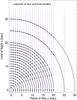 |
Fig. 10 Illustration of the used shell and ray structure including the cutpoints. Moving inward more and more shell contributions enter the observed surface brightness. |
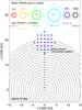 |
Fig. 11 Comparison of the shell structure and the telescope beams at the different wavelengths. The size of the beam (approximated by a Gaussian with the variance σ2) is illustrated both by the full width half maximum (FWHM) and 2σ circles. Gaussian convolutions are performed using a 29 point stencil shown in the figure center. |
This approach differs from the inverse RT used in R+14 based on an Abel transform inverting the problem directly providing the unknown density and temperature. This method can also be generalized to elliptical shells. Particular differences in the modeling are:
-
Forward ray-tracing does not require to smear all maps to the same (coarse) resolution of the 500 μm maps which causes a loss of spatial information especially in the central parts. Instead individual beam smearing is performed after the theoretical radiation field has been determined from the chosen temperature and density grid.
-
R+14 derive their density and temperature profiles from azimuthally averaged surface brightness, and use the deviations from the average along different directions to estimate uncertainties in their profiles. With this approach, it is not clear how to define a radius where the core ends and where the model is averaging filament matter with non-related low density matter outside the core-filament system. The substantial alteration of the observed surface brightness by the azimuthal average is illustrated in Fig. 12. The observed 250 μm map is compared to the same map with direction-averaging out to 35 kau as in R+14. In contrast, our core-filament border estimates in Sect. 2.1 point to 9 to 15 kau as the outer core radius.
-
The central part of the core is the most interesting region in terms of the basic unanswered questions about the onset of star formation. It also hosts the coldest dust in the system which by the simple formalism of black body radiation is hardest to see (a drop of 1 K decreases the maximal Planck radiation by a factor of 2 due to its T5-dependence). The uncertainty in the density and temperature arising from this lack of sensitivity is described in the next section.
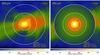 |
Fig. 12 Herschel 250 μm map of L1689B (left) and the strong alteration by an azimuthal average as performed in the R+14 model (right), mixing filament, core, and filament-external contributions. White circles indicate various radial distances from the center. |
4. Deriving the density and temperature structure along the western cut
4.1. Grid calculations for the inner shells
There are a few circumstances that make the detection of cold dust in the core center more difficult. Lines of sight through the center always see emission from all layers. In competition with the outer warm (>10 K) and thus brighter dust, the colder central dust must compensate with a higher density to become observable. Moreover, because of the limited angular resolution of smaller telescopes like Herschel, the flux coming from warm and cold regions is spatially averaged, and gradients are smoothed out, especially at longer wavelengths like 500 μm. Consequently, ground-based observations at longer wavelengths with larger telescopes that have a smaller beam are better probing the central region.
To determine the density and temperature structure along the Western cut of the core, we have treated separately the inner five shells (spanning 5 kau in radius) and the outer shells beyond 5 kau. For the outer region, we used the exponential approximations of the observed surface brightness as shown in Fig. 6 down to 6 kau, and applied the method described in Sect. 3. For the inner shells, for which convolution with the telescope beam has to be taken into account we have run forward radiative transfer over a full grid of densities and temperatures with 10 values in each of the 10 parameters (5 densities and 5 temperatures), deriving in each case the intensity after convolution with the appropriate beam. Since the precise shape of the error distributions of the observed surface brightnesses is not known, we have taken the simple approach to accepted all solutions fitting all surface brightness profiles simultaneously within the calibration errors of the bands estimated to be 10% for SPIRE, 15% for PACS, and 30% for SCUBA-2, see Bacmann et al. (2016). For the sake of comparison, we have the same dust opacities as R+14 (HGBS opacities, and a gas-to-dust ratio 100).
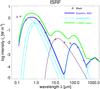 |
Fig. 13 Standard interstellar radiation field for a low-mass star formation region (blue) after Zucconi et al. (2001) with its different components as magenta lines. For comparison, points from the Black (1994) field are shown as plus signs. A mid-infrared component was added (thin black line) to arrive at these values. The green line gives the local ISRF of L1689B. |
4.2. Grid calculations for the outer interstellar radiation field
For the inner shells, we found a range of density and temperature profiles consistent with the data. Indeed, increasing the central density (and hence obtaining a steeper profile) can be compensated by lowering the temperature. However, solutions for the temperature profile should be consistent with a temperature profile obtained by calculating the propagation of interstellar radiation through the corresponding density structure. Hence, we have designed a new synergetic RT approach. Since we determined the outer (>5 kau) density and temperature structure, we can use this information to estimate the outer radiation field. The ISRF was parameterized following the approach by Zucconi et al. (2001) based on the work by Black (1994). Figure 13 presents their ISRF spectrum (blue) composed of the individual components (magenta) and the Black (1994) data (black crosses). As pointed out by Zucconi et al. (2001), their ISRF is a minimal field not containing the likely addition of a mid-infrared (MIR) component due to warm dust in star formation regions. We therefore added this component (thin black) to reproduce the Black (1994) data. Based on this ISRF we have run a large grid of RT calculations determining a new temperature profile using the density structure derived for L1689B by “peeling” RT, as described in Sect. 3. We used the standard dust opacities by Draine & Lee (1984) which we merged into the HGBS opacities in the FIR and submillimeter for consistency. In each run we have varied each of the components of the ISRF by factors ranging from 0.1 to 10: stellar (first three components), warm dust (peaking around 10 μm), and cold dust (peaking around 100 μm). The spread in possible ISRFs fitting both the peeling RT temperature profile and the observed surface brightness profiles was narrow. The ISRF near L1689B is best described by an ISRF with twice the stellar component and four times the warm and cold dust components (green).
Based on this local ISRF for L1689B, we have re-calculated also the temperature of the inner five shells for each of the formerly derived density profiles. By accepting only solutions where the two differently derived temperatures match, we were able to extract the solution subspace that contains density and temperature profiles both fitting all surface brightness profiles and being consistent with a single outer ISRF.
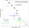 |
Fig. 14 H2 number density-dust temperature for the five inner shells of L1689B with a size of 1 kau each. The crosses mark the ranges for which all profiles can be fitted within the calibration errors simultaneously. The dots represent the mean values from R+14. For the inner shell, n-T pairs are possible along an exponential function (A = 6.4 × 10¹⁴ m-3 and a = 1.4 K). The grey lower limit indicates densities which are compatible with line emission modeling as mentioned in Sect. 5. |
Figure 14 shows the corresponding density-temperature solution space (hereafter n-T) for each of the five inner shells (color-coded) as crosses. In the two inner shells (blue and black) some ambiguity remains: in the second shell the temperature (density) ranges between 7.5 and 9.6 K (2 × 10¹¹ m-3 and 5.8 × 10¹¹ m-3), respectively – lower in temperature and higher in density than values from the mean R+14 (dots). We note that the mean R+14 values are an average while they also performed fits along individual cuts. But since these individual profiles were only used in the error bars we rely on the mean values here. In the inner shell, any pair of n and T values obeying the relation n = Aexp(T/a) (A = 6.4 × 10¹⁴ m-3 and a = 1.4 K) – is still be consistent with the data and the ISRF. Our solution includes densities above 1012 m-3 for temperatures <9 K. Physically, the ambiguity reflects the fact that with all the warmer shells contributing to the central line-of-sight, the additional cold dust emission contribution can be kept constant when a higher density is compensated with lower temperature. The ambiguity is increased when beam-convolution is performed or the maps are smoothed to the coarse spatial resolution of the 500 μm Herschel observations.
The resulting H2 number density profile is shown in Fig. 15 (black solid) along with the R+14 profile (blue), and an r-2-profile (dotted). For the inner cells, the density values fitting all surface brightness profiles within the calibration errors are indicated as green bars. With the constraints derived from the ISRF, the ranges shrink to the black bars. For the inner cell, the bar is plotted dashed to indicate that each density within the range is correlated with the temperature following the exponential relation visible in Fig. 14 for high densities.
With a similar color code, we show the dust temperature profile in Fig. 16. The temperatures are lower than the R+14 mean values, and can decrease to about 6.8 K in the inner cell.
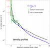 |
Fig. 15 H2 number density profile for L1689B (black solid). Like the profile from R+14 (blue) the outer core parts approximately follow an r-2 law but arrive at higher central densities. The remaining ambiguity in the inner cell is shown by green bars. The n-T-relation of possible inner shell solutions is marked with a dashed bar giving the corresponding temperatures. |
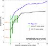 |
Fig. 16 Dust temperature profile for L1689B (black solid). The temperatures are lower than those of R+14. The notation is the same as in Fig. 15. |
5. Discussion
In this section, we discuss a number of implications based on our new density and temperature profiles in compact subsections.
5.1. Strength of the interstellar radiation field: the standard ISRF amplified by a factor of 10 is too high
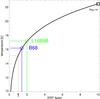 |
Fig. 17 Temperature of dust fully exposed to the radiation field as a function the amplification factor of the standard interstellar radiation field. |
In view of the obtained relatively high central temperature of L1689B of 9.8 ± 0.5 K R+14 argued that the radiation field near the core may be a factor of 10 stronger than the standard ISRF due to the presence of early-type stars in the vicinity of the main (L1688) Ophiuchus cloud as treated in Liseau et al. (1999). This factor might however not apply to the L1689 cloud, which is located further away from these stars. A simple calculation can be made for the temperature of the dust that is on the outskirts of the filament and therefore well-exposed to the complete radiation field.
Figure 17 presents the temperature of the dust which is fully exposed to a scaled-up standard ISRF as a function of the scaling factor. The outer temperature near L1689B and B68 can easily be derived from the maps obtained by pixel-by-pixel single temperature SED fitting in R+14 or in Sect. 5.3. This enables us to determine the ISRF scaling factors to account for the outer temperatures in B68 and L1689B, 1.5 and 2, respectively. The value of 2 shown in the figure for L1689B is consistent with the more precisely determined ISRF in Sect. 4.2 of the present work with factors of 2 (stellar), 4 (warm dust), and 4 (cold dust) since the outer dust is mainly heated by the stellar component. ISRFs ten times higher would heat the dust to about 22.5 K which is not observed near L1689B.
5.2. Mass and central column density: a denser center
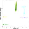 |
Fig. 18 Correlation between the central H2 column number density and the core mass of L1689B. Aside of various ranges from the literature, the solution space found in this work is shown color-coding the number of solutions at about 7 M⊙. The distribution has a longer extent in column density since it is more affected by the dense inner shells than the mass. |
The variation in derived column densities and especially in masses as mentioned in the introduction is shown in Fig. 18 along with the our modeling result (both fitting all profiles and consistent with a single ISRF). We have color-coded the number of solutions which all are located near 7 M⊙ in mass. As the inner dense shells impact the column density much more than the mass, the spread in possible column densities is larger and extend well above the values discussed so far. The R+14 core mass is too high as it includes filament contributions. We note that we have used the same dust opacities and source distance to exclude potential differences from these assumptions. A similar argument applies for the mass estimate by Bacmann et al. (2000) based on an outer radius of 28 kau. Their opacities are near the HGBS values used in our work, but they assumed a distance of 160 pc instead of 140 pc which increase the mass by about 30%. Kirk et al. (2005) and Makiwa et al. (2016) used slightly smaller distances (130 pc and 120 pc, respectively) but again comparable opacities, and nevertheless derived much smaller masses. Their estimates likely suffer from the single-fit approximation as shown in the next subsection.
5.3. Pixel-by-pixel single temperature SED fits do not work for dense cores
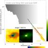 |
Fig. 19 Line-of-sight H2 column number density and temperature for the pixel-by-pixel single temperature SED fit (points along the line, temperature and column density map shown as inlet). The grey-scaled region shows the area where all model column densities and temperature solutions are located (the color-coding is based on the logarithmic density at the various temperatures entering the column density). |
Especially in the first Herschel data releases, pixel-by-pixel single temperature SED fits of regions with cores have been presented (e.g., Könyves et al. 2010). They have turned out to be helpful in characterizing the core environment where the single temperature assumption is valid, because of the low densities. Figure 19 shows the temperature and column density maps based on single-temperature SED fitting of the L1689B continuum data as inlet. Clearly, the two maps are correlated in structure, and indeed the column density-temperature relation shown is surprisingly narrow (the color coding refers to the temperature). The relation covers cloud dust (yellow), filament dust (orange) and core dust (green to black). The maximal (minimal) column densities (temperatures) are far from the values arising from our detailed modeling with a temperature and density variation along the line-of-sight. The full range of possible pairs of the two quantities is shown in grey. This means that neither a single temperature is a good approximation for lines intersecting a dense core, nor does such an analysis produce reliable central column densities or temperatures.
5.4. Core mass functions, or are they filament mass functions too?
Estimating masses has proven to be a difficult task for star-forming cores. The uncertainty in the dust properties and the complex topologies of the density are just two of the major obstacles encountered. Correspondingly, core mass functions (CMF) carry large error bars on top of potential biases from incompleteness. In this work, we point out two more potential problems namely the inclusion of too much filament mass, and the break-down of the single temperature approximation that yield too low masses and central column densities. From our analysis, the critical point is not only to limit the mass calculation within smaller radii, close to the border between core and filament, but also to avoid adding the contribution of the filament in front and behind along the line-of-sight. The Abel inversion method based on azimuthally averaged shells or ellipsoids described in R+14 is therefore not well suited to mass determination for the CMF.
5.5. Variation of the results when altering the dust properties
In general, the derived densities scale with the overall shift in FIR absorption cross sections when another dust model is used. This uncertainty remains until we can find out more about the physical nature of the dust near and in the core. As a side note we mention here that the surface brightness modeling of the 500 μm profiles provided better fits when lowering the HGBS opacity by 15%. This is not to be confused with an offset problem of the filter which would add a constant offset while the offset we find is a factor. For us this may point to a deviation in the opacity of the dust in L1689B.
The choice of dust opacity becomes even more relevant in the core center where coagulation calculations hint at a growth of grains (Ossenkopf & Henning 1994), extinction measurements indicate a flattening in the extinction law (e.g., McClure 2009), and scattered MIR radiation seems to indicate the presence of μm-sized grains (Steinacker et al. 2010). The existing Spitzer images of L1689B at 3.6 μm are difficult to interpret because of the presence of a nearby bright star, and the existence of coreshine as scattered light from large grains can not be assessed. However, current coreshine measurements in prestellar cores seem to speak against a strong variation in dust properties on scales of 10 kau (Andersen et al. 2013).
5.6. Very cold dust (<8 K) has a small mass percentage in L1689B
Our exploration of the parameter space for the inner shells have not produced solutions where dust with temperatures below 8 K is found outside the two inner cells. While the contribution of these two shells to the column density are substantial and cause the remaining spread in our central temperature estimates, their contribution to the core mass in L1689B is small (<10%) and far from the 30−70 estimated by Pagani et al. (2015).
This latter work also mentions preliminary modeling of emission line data which requires central H2 number densities above ~2 × 10¹² m-3 as indicated in Fig. 14. The presented range of values for the central shell includes these densities and the correlation found between density and temperature for this solution branch can actually be used in the modeling now.
Provided with a detailed description about the observations and data reductions at http://gouldbelt-herschel.cea.fr/archives
Acknowledgments
We thank A. Roy and P. Palmeirim for providing the Abel transform profile data. The anonymous referee we thank for a number of constructive comments helping to improve the manuscript. This research has made use of data from the Herschel Gould Belt survey (HGBS) project (http://gouldbelt-herschel.cea.fr). The HGBS is a Herschel key programme jointly carried out by SPIRE Specialist Astronomy Group 3 (SAG 3), scientists of several institutes in the PACS Consortium (CEA Saclay, INAF-IFSI Rome and INAF-Arcetri, KU Leuven, MPIA Heidelberg), and scientists of the Herschel Science Center (HSC). Herschel is an ESA space observatory with science instruments provided by European-led Principal Investigator consortia and with important participation from NASA. SPIRE has been developed by a consortium of institutes led by Cardiff Univ. (UK) and including Univ. Lethbridge (Canada); NAOC (China); CEA, LAM (France); IFSI, Univ. Padua (Italy); IAC (Spain); Stockholm Observatory (Sweden); Imperial College London, RAL, UCL-MSSL, UKATC, Univ. Sussex (UK); Caltech, JPL, NHSC, Univ. Colorado (USA). This development has been supported by national funding agencies: CSA (Canada); NAOC (China); CEA, CNES, CNRS (France); ASI (Italy); MCINN (Spain); SNSB (Sweden); STFC (UK); and NASA (USA). PACS has been developed by a consortium of institutes led by MPE (Germany) and including UVIE (Austria); KUL, CSL, IMEC (Belgium); CEA, OAMP (France); MPIA (Germany); IFSI, OAP/AOT, OAA/CAISMI, LENS, SISSA (Italy); IAC (Spain). This development has been supported by the funding agencies BMVIT (Austria), ESA-PRODEX (Belgium), CEA/CNES (France), DLR (Germany), ASI (Italy), and CICT/MCT (Spain). The James Clerk Maxwell Telescope has historically been operated by the Joint Astronomy Centre on behalf of the Science and Technology Facilities Council of the United Kingdom, the National Research Council of Canada and the Netherlands Organisation for Scientific Research. Additional funds for the construction of SCUBA-2 were provided by the Canada Foundation for Innovation. IRAM is supported by INSU/CNRS (France), MPG (Germany) and IGN (Spain). This research has made use of NASA’s Astrophysics Data System.
References
- Alves, J. F., Lada, C. J., & Lada, E. A. 2001, Nature, 409, 159 [NASA ADS] [CrossRef] [PubMed] [Google Scholar]
- Andersen, M., Steinacker, J., Thi, W.-F., et al. 2013, A&A, 559, A60 [NASA ADS] [CrossRef] [EDP Sciences] [Google Scholar]
- Andre, P., Ward-Thompson, D., & Motte, F. 1996, A&A, 314, 625 [NASA ADS] [Google Scholar]
- André, P., Men’shchikov, A., Bontemps, S., et al. 2010, A&A, 518, L102 [NASA ADS] [CrossRef] [EDP Sciences] [Google Scholar]
- André, P., Di Francesco, J., Ward-Thompson, D., et al. 2014, Protostars and Planets VI, 27 [Google Scholar]
- Bacmann, A., André, P., Puget, J.-L., et al. 2000, A&A, 361, 555 [Google Scholar]
- Bacmann, A., Daniel, F., Caselli, P., et al. 2016, A&A, 587, A26 [NASA ADS] [CrossRef] [EDP Sciences] [Google Scholar]
- Bergin, E. A., & Tafalla, M. 2007, ARA&A, 45, 339 [NASA ADS] [CrossRef] [Google Scholar]
- Black, J. H. 1994, in The First Symposium on the Infrared Cirrus and Diffuse Interstellar Clouds, eds. R. M. Cutri, & W. B. Latter, ASP Conf. Ser., 58, 355 [Google Scholar]
- Broderick, A. E., & Keto, E. 2010, ApJ, 721, 493 [NASA ADS] [CrossRef] [Google Scholar]
- Crapsi, A., Caselli, P., Walmsley, C. M., et al. 2005, ApJ, 619, 379 [Google Scholar]
- Draine, B. T., & Lee, H. M. 1984, ApJ, 285, 89 [Google Scholar]
- Fischera, J., & Martin, P. G. 2012, A&A, 542, A77 [NASA ADS] [CrossRef] [EDP Sciences] [Google Scholar]
- Gregersen, E. M., & Evans, II, N. J. 2000, ApJ, 538, 260 [NASA ADS] [CrossRef] [Google Scholar]
- Griffin, M. J., Abergel, A., Abreu, A., et al. 2010, A&A, 518, L3 [Google Scholar]
- Hacar, A., & Tafalla, M. 2011, A&A, 533, A34 [NASA ADS] [CrossRef] [EDP Sciences] [Google Scholar]
- Hacar, A., Tafalla, M., Kauffmann, J., & Kovács, A. 2013, A&A, 554, A55 [NASA ADS] [CrossRef] [EDP Sciences] [Google Scholar]
- Heigl, S., Burkert, A., & Hacar, A. 2016, ArXiv e-prints [arXiv:1601.02018] [Google Scholar]
- Hennebelle, P. 2003, A&A, 411, 9 [NASA ADS] [CrossRef] [EDP Sciences] [Google Scholar]
- Jessop, N. E., & Ward-Thompson, D. 2001, MNRAS, 323, 1025 [NASA ADS] [CrossRef] [Google Scholar]
- Keto, E., & Caselli, P. 2010, MNRAS, 402, 1625 [NASA ADS] [CrossRef] [Google Scholar]
- Kirk, J. M., Ward-Thompson, D., & André, P. 2005, MNRAS, 360, 1506 [NASA ADS] [CrossRef] [Google Scholar]
- Könyves, V., André, P., Men’shchikov, A., et al. 2010, A&A, 518, L106 [NASA ADS] [CrossRef] [EDP Sciences] [Google Scholar]
- Lada, C. J., Bergin, E. A., Alves, J. F., & Huard, T. L. 2003, ApJ, 586, 286 [NASA ADS] [CrossRef] [Google Scholar]
- Launhardt, R., Stutz, A. M., Schmiedeke, A., et al. 2013, A&A, 551, A98 [NASA ADS] [CrossRef] [EDP Sciences] [Google Scholar]
- Lee, C. W., Myers, P. C., & Tafalla, M. 2001, ApJS, 136, 703 [NASA ADS] [CrossRef] [Google Scholar]
- Liseau, R., White, G. J., Larsson, B., et al. 1999, A&A, 344, 342 [NASA ADS] [Google Scholar]
- Loinard, L., Torres, R. M., Mioduszewski, A. J., & Rodríguez, L. F. 2008, ApJ, 675, L29 [NASA ADS] [CrossRef] [Google Scholar]
- Lombardi, M., Lada, C. J., & Alves, J. 2008, A&A, 480, 785 [NASA ADS] [CrossRef] [EDP Sciences] [Google Scholar]
- Makiwa, G., Naylor, D. A., van der Wiel, M. H. D., et al. 2016, MNRAS, 458, 2150 [NASA ADS] [CrossRef] [Google Scholar]
- Malinen, J., Juvela, M., Rawlings, M. G., et al. 2012, A&A, 544, A50 [NASA ADS] [CrossRef] [EDP Sciences] [Google Scholar]
- Maret, S., Bergin, E. A., & Tafalla, M. 2013, A&A, 559, A53 [NASA ADS] [CrossRef] [EDP Sciences] [Google Scholar]
- Marsh, K. A., Kirk, J. M., André, P., et al. 2016, MNRAS, 459, 342 [NASA ADS] [CrossRef] [Google Scholar]
- McClure, M. 2009, ApJ, 693, L81 [NASA ADS] [CrossRef] [Google Scholar]
- McLaughlin, D. E., & Pudritz, R. E. 1996, ApJ, 469, 194 [NASA ADS] [CrossRef] [Google Scholar]
- Nielbock, M., Launhardt, R., Steinacker, J., et al. 2012, A&A, 547, A11 [NASA ADS] [CrossRef] [EDP Sciences] [Google Scholar]
- Ossenkopf, V., & Henning, T. 1994, A&A, 291, 943 [NASA ADS] [Google Scholar]
- Ostriker, J. 1964, ApJ, 140, 1056 [NASA ADS] [CrossRef] [MathSciNet] [Google Scholar]
- Pagani, L., Lefèvre, C., Juvela, M., Pelkonen, V.-M., & Schuller, F. 2015, A&A, 574, L5 [NASA ADS] [CrossRef] [EDP Sciences] [Google Scholar]
- Palmeirim, P., André, P., Kirk, J., et al. 2013, A&A, 550, A38 [NASA ADS] [CrossRef] [EDP Sciences] [Google Scholar]
- Pattle, K., Ward-Thompson, D., Kirk, J. M., et al. 2015, MNRAS, 450, 1094 [NASA ADS] [CrossRef] [Google Scholar]
- Redman, M. P., Keto, E., Rawlings, J. M. C., & Williams, D. A. 2004, MNRAS, 352, 1365 [NASA ADS] [CrossRef] [Google Scholar]
- Roy, A., André, P., Palmeirim, P., et al. 2014, A&A, 562, A138 [NASA ADS] [CrossRef] [EDP Sciences] [Google Scholar]
- Schmalzl, M., Launhardt, R., Stutz, A. M., et al. 2014, A&A, 569, A7 [NASA ADS] [CrossRef] [EDP Sciences] [Google Scholar]
- Schnee, S., Brunetti, N., Di Francesco, J., et al. 2013, ApJ, 777, 121 [NASA ADS] [CrossRef] [Google Scholar]
- Seo, Y. M., Hong, S. S., & Shirley, Y. L. 2013, ApJ, 769, 50 [NASA ADS] [CrossRef] [Google Scholar]
- Shu, F. H. 1977, ApJ, 214, 488 [NASA ADS] [CrossRef] [Google Scholar]
- Smith, R. J., Shetty, R., Stutz, A. M., & Klessen, R. S. 2012, ApJ, 750, 64 [NASA ADS] [CrossRef] [Google Scholar]
- Smith, R. J., Glover, S. C. O., & Klessen, R. S. 2014, MNRAS, 445, 2900 [NASA ADS] [CrossRef] [Google Scholar]
- Steinacker, J., Pagani, L., Bacmann, A., & Guieu, S. 2010, A&A, 511, A9 [NASA ADS] [CrossRef] [EDP Sciences] [Google Scholar]
- Teyssier, R. 2002, A&A, 385, 337 [NASA ADS] [CrossRef] [EDP Sciences] [Google Scholar]
- Tilley, D. A., & Pudritz, R. E. 2003, ApJ, 593, 426 [NASA ADS] [CrossRef] [Google Scholar]
- Ward-Thompson, D., Di Francesco, J., Hatchell, J., et al. 2007, PASP, 119, 855 [NASA ADS] [CrossRef] [Google Scholar]
- Zucconi, A., Walmsley, C. M., & Galli, D. 2001, A&A, 376, 650 [NASA ADS] [CrossRef] [EDP Sciences] [Google Scholar]
All Figures
|
Fig. 1 Contours where the intensity of the core reaches the filament maximal intensity (reference point between the two vertical sub-filaments) for the different wavelengths. The color-coded image shows the 160 μm map. |
| In the text | |
|
Fig. 2 Cut through the H2 number density structure including the core center for a hydro-dynamical simulation of the evolution of a filament with the RAMSES code. The white circle indicates the radius where the density deviation from spherical symmetry exceeds 50%. |
| In the text | |
|
Fig. 3 Cuts through the H2 number density RAMSES results along the filament axis (thick black), with the maximal filament density subtracted (thick, dashed), and perpendicular to the filament axis (orange). The thin solid line indicates the steepness of a powerlaw with the exponent −1.73 which approximates the dashed line in a region around 10 kau. |
| In the text | |
|
Fig. 4 Sketch of the horizontal cut along the filament main axis in the plane-of-sky. The cut has a height corresponding to the beam size at the considered wavelengths. The density in the plane of lines-of-sight is indicated in grey-scale along with the shells of the spherical density model. |
| In the text | |
|
Fig. 5 Surface representation of the L1689B Herschel PACS map at 160 μm amplifying the substructure. The main filament axis is rotated horizontally and the core is in the center. Two narrow filaments are visible on the right perpendicular to the main filament, and the filament shows a narrow substructure along the main filament axis west of the core. There is also sub-structure visible in the central core region at this wavelength. |
| In the text | |
|
Fig. 6 Left and middle: radial cuts of the Herschel maps of L1689B in western direction from the core center. The numbers indicate the wavelength. Calibration error bars are added for the middle panel. The exponential shape of the 850 μm profile is better visible in the lin-log representation. The horizontal thin lines indicates the offset surface brightness from the filament. The two thin blue lines estimate the slope variation in the 800 μm-profile. Right: after subtracting the offsets, all profiles are close to an exponential function with approximately the same exponent A. The dotted lines show the exponential function with A = 0.11. The dashed vertical lines give the distance where deviations from the exponential occur. |
| In the text | |
|
Fig. 7 Line-of-sight integral through an iso-thermal sphere (solid) can be approximated in large parts by an exponential (dotted). |
| In the text | |
|
Fig. 8 Offset-subtracted surface brightness profiles for the Eastern cut along the filament axis (thick) in comparison to the Western cut (thin dashed, Fig. 6). The exponential fit leads to steeper gradients (A = 0.14) than for the Western cut. The surface brightnesses at 160 and 250 μm are enhanced due to a vertical filament in the region around 20 kau distance. |
| In the text | |
|
Fig. 9 Vertical surface brightness profiles (y direction) in the 250 μm map in three boxes left, central, and right around the core. The left box shows the narrow filament maximum (indicated again in the middle box as yellow line). The right box shows a broader maximum (at about the same level, see brown line in the middle box). The central cuts are shown as white lines in the middle box. Dotted circles indicate the distance from the center. |
| In the text | |
|
Fig. 10 Illustration of the used shell and ray structure including the cutpoints. Moving inward more and more shell contributions enter the observed surface brightness. |
| In the text | |
|
Fig. 11 Comparison of the shell structure and the telescope beams at the different wavelengths. The size of the beam (approximated by a Gaussian with the variance σ2) is illustrated both by the full width half maximum (FWHM) and 2σ circles. Gaussian convolutions are performed using a 29 point stencil shown in the figure center. |
| In the text | |
|
Fig. 12 Herschel 250 μm map of L1689B (left) and the strong alteration by an azimuthal average as performed in the R+14 model (right), mixing filament, core, and filament-external contributions. White circles indicate various radial distances from the center. |
| In the text | |
|
Fig. 13 Standard interstellar radiation field for a low-mass star formation region (blue) after Zucconi et al. (2001) with its different components as magenta lines. For comparison, points from the Black (1994) field are shown as plus signs. A mid-infrared component was added (thin black line) to arrive at these values. The green line gives the local ISRF of L1689B. |
| In the text | |
|
Fig. 14 H2 number density-dust temperature for the five inner shells of L1689B with a size of 1 kau each. The crosses mark the ranges for which all profiles can be fitted within the calibration errors simultaneously. The dots represent the mean values from R+14. For the inner shell, n-T pairs are possible along an exponential function (A = 6.4 × 10¹⁴ m-3 and a = 1.4 K). The grey lower limit indicates densities which are compatible with line emission modeling as mentioned in Sect. 5. |
| In the text | |
|
Fig. 15 H2 number density profile for L1689B (black solid). Like the profile from R+14 (blue) the outer core parts approximately follow an r-2 law but arrive at higher central densities. The remaining ambiguity in the inner cell is shown by green bars. The n-T-relation of possible inner shell solutions is marked with a dashed bar giving the corresponding temperatures. |
| In the text | |
|
Fig. 16 Dust temperature profile for L1689B (black solid). The temperatures are lower than those of R+14. The notation is the same as in Fig. 15. |
| In the text | |
|
Fig. 17 Temperature of dust fully exposed to the radiation field as a function the amplification factor of the standard interstellar radiation field. |
| In the text | |
|
Fig. 18 Correlation between the central H2 column number density and the core mass of L1689B. Aside of various ranges from the literature, the solution space found in this work is shown color-coding the number of solutions at about 7 M⊙. The distribution has a longer extent in column density since it is more affected by the dense inner shells than the mass. |
| In the text | |
|
Fig. 19 Line-of-sight H2 column number density and temperature for the pixel-by-pixel single temperature SED fit (points along the line, temperature and column density map shown as inlet). The grey-scaled region shows the area where all model column densities and temperature solutions are located (the color-coding is based on the logarithmic density at the various temperatures entering the column density). |
| In the text | |
Current usage metrics show cumulative count of Article Views (full-text article views including HTML views, PDF and ePub downloads, according to the available data) and Abstracts Views on Vision4Press platform.
Data correspond to usage on the plateform after 2015. The current usage metrics is available 48-96 hours after online publication and is updated daily on week days.
Initial download of the metrics may take a while.