| Issue |
A&A
Volume 593, September 2016
|
|
|---|---|---|
| Article Number | A49 | |
| Number of page(s) | 15 | |
| Section | Interstellar and circumstellar matter | |
| DOI | https://doi.org/10.1051/0004-6361/201628588 | |
| Published online | 15 September 2016 | |
Binary system and jet precession and expansion in G35.20–0.74N⋆
1 INAF–Osservatorio Astrofisico di
Arcetri, Largo E. Fermi 5, 50125 Firenze, Italy
e-mail: This email address is being protected from spambots. You need JavaScript enabled to view it.
2 I. Physikalisches Institut,
Universität zu Köln, Zülpicher Str.
77, 50937
Köln,
Germany
3 National Astronomical Observatory of
Japan, Mitaka,
Tokyo
181-8588,
Japan
4 Department of Astronomical Sciences,
SOKENDAI (The Graduate University for Advanced Studies), Mitaka, Tokyo
181-8588,
Japan
5 Centre for Astrophysics, University
of Hertfordshire, College
Lane, Hatfield,
AL10 9AB,
UK
6 Instituto de Astrofísica e Ciências
do Espaço, Universidade do Porto, CAUP, Rua das Estrelas, 4150-762
Porto,
Portugal
Received:
24
March
2016
Accepted:
13
June
2016
Abstract
Context. Atacama Large Millimeter/submillimeter Array (ALMA) observations of the high-mass star-forming region G35.20−0.74N have revealed the presence of a Keplerian disk in core B rotating about a massive object of 18 M⊙, as computed from the velocity field. The luminosity of such a massive star would be comparable to (or higher than) the luminosity of the whole star-forming region. To solve this problem it has been proposed that core B could harbor a binary system. This could also explain the possible precession of the radio jet associated with this core, which has been suggested by its S-shaped morphology.
Aims. We establish the origin of the free-free emission from core B and investigate the existence of a binary system at the center of this massive core and the possible precession of the radio jet.
Methods. We carried out VLA continuum observations of G35.20−0.74N at 2 cm in the B configuration and at 1.3 cm and 7 mm in the A and B configurations. The bandwidth at 7 mm covers the CH3OH maser line at 44.069 GHz. Continuum images at 6 and 3.6 cm in the A configuration were obtained from the VLA archive. We also carried out VERA observations of the H2O maser line at 22.235 GHz.
Results. The observations have revealed the presence of a binary system of UC/HC Hii regions at the geometrical center of the radio jet in G35.20−0.74N. This binary system, which is associated with a Keplerian rotating disk, consists of two B-type stars of 11 and 6 M⊙. The S-shaped morphology of the radio jet has been successfully explained as being due to precession produced by the binary system. The analysis of the precession of the radio jet has allowed us to better interpret the IR emission in the region, which would be not tracing a wide-angle cavity open by a single outflow with a position angle of ~55°, but two different flows: a precessing one in the NE–SW direction associated with the radio jet, and a second one in an almost E–W direction. Comparison of the radio jet images obtained at different epochs suggests that the jet is expanding at a maximum speed on the plane of the sky of 300 km s-1. The proper motions of the H2O maser spots measured in the region also indicate expansion in a direction similar to that of the radio jet.
Conclusions. We have revealed a binary system of high-mass young stellar objects embedded in the rotating disk in G35.20−0.74N. The presence of a massive binary system is in agreement with the theoretical predictions of high-mass star formation, according to which the gravitational instabilities during the collapse would produce the fragmentation of the disk and the formation of such a system. For the first time, we have detected a high-mass young star associated with an UC/HC Hii region and at the same time powering a radio jet.
Key words: ISM: individual objects: G35.20-0.74N / Hii regions / ISM: jets and outflows / stars: formation
The reduced images (FITS files) is only available at the CDS via anonymous ftp to cdsarc.u-strasbg.fr (130.79.128.5) or via http://cdsarc.u-strasbg.fr/viz-bin/qcat?J/A+A/593/A49
© ESO, 2016
1. Introduction
The discovery of circumstellar disks around early B-type stars (e.g., Beltrán & de Wit 2015 and references therein) in recent years has led to a big leap in our understanding of high-mass star formation. It shows that B-stars form via disk-mediated accretion confirming the predictions of theoretical models (Bonnell & Bate 2006; Keto 2007; Krumholz et al. 2009). But theoretical predictions go further and suggest that gravitational instabilities during the collapse would cause the disk to fragment, resulting in massive binary, triple or multiple systems, depending on the initial mass of the cloud (Krumholz et al. 2009). Young high-mass binary or multiple systems have been very elusive till now with only a few convincing candidates (e.g., Shepherd et al. 2001). Next, although molecular outflows are ubiquitously found in both low- and high-mass stars, thermal ionized jets – common in low-mass protostars – have so far been found in association with only a handful of outflows driven by high-mass young stellar objects (YSOs; e.g., Guzmán et al. 2012). What is more, no thermal radio jet known to be driven by a high-mass YSO associated with an Hii region has ever been found.
Parameters of the maps.
In a progressive effort to understand massive star formation and verify the predictions of theoretical models, we performed Atacama Large Millimeter/submillimeter Array (ALMA) observations of star-forming regions hosting B-type stars. One of our targets was the well-known high-mass YSO G35.20−0.74N (hereafter G35.20N), which is located at 2.2 kpc (Zhang et al. 2009) and has a luminosity of ~3 × 10⁴L⊙. This star-forming region is characterized by the presence of a butterfly-shaped nebula, imaged at IR wavelengths, roughly coinciding with a poorly collimated wide-angle bipolar outflow oriented NE–SW (Gibb et al. 2003; Qiu et al. 2013). Radio and IR images reveal the presence of a collimated N–S jet (Sánchez-Monge et al. 2013, 2014) originating from the same center as the bipolar nebula and lying along the western border of the wide-angle bipolar nebula/outflow. It has been suggested that the jet could be precessing around the NE–SW direction, and be responsible for the bipolar structure.
The ALMA observations have uncovered at least five cores across the waist of this bipolar nebula (Sánchez-Monge et al. 2014), one of which (core B) appears to drive the N–S jet (Sánchez-Monge et al. 2013). This core is spatially elongated and shows a velocity gradient perpendicular to the axis of the bipolar nebula. Sánchez-Monge et al. (2013) demonstrate that the velocity field of the core can be fitted with a Keplerian disk rotating about a massive object of 18 M⊙. Such a mass is unlikely to be concentrated in a single star because the luminosity of an 18 M⊙ star is comparable to the bolometric luminosity of the entire G35.20N star-forming region. To solve this luminosity problem, it has been argued that the luminosity of the region could have been underestimated if part of the stellar radiation had escaped through the outflow cavities (Zhang et al. 2013). Alternatively, the measured luminosity (3 × 10⁴L⊙) could arise from more than one lower luminosity/mass star. This solution led Sánchez-Monge et al. (2013) to argue that the 18 M⊙ unresolved object consists of a binary system, with individual luminosities that can be as low as ~7000 L⊙. The existence of a binary could cause precession of the jet about the NE–SW axis of the disk, consistent with the scenario depicted above for the origin of the bipolar nebula.
The next intriguing feature of core B is the presence of an unresolved free-free emission source inside this core. This source seems to be part of the N–S radio jet, but has a spectral index α>1.3 (Sν ∝ να) between 6 and 3.6 cm (Gibb et al. 2003), and ~1.8 between 3.6 and 1.3 cm (Codella et al. 2010), compatible with optically thick free-free emission from an Hii region (α ~ 2). In contrast, thermal radio jets have typically weak continuum fluxes of a few mJy and α = 1.3−0.7/ϵ ≲ 1.3, where ϵ is related to the collimation of the jet (for a prototypical biconical jet ϵ = 1 and α = 0.6: Reynolds 1986; Anglada 1996). While the Hii region scenario appears to be compatible with the measured spectral indices, it cannot rule out the possibility that the free-free emission from core B originates in the N–S thermal jet because the observations at different wavelengths have been performed with different angular resolutions. This makes it difficult to reliably estimate the spectral index (3.6 cm and 6 cm:  –
– ; 1.3 cm:
  ).
).
To establish the origin of the free-free emission from core B and test the hypothesis of a binary system in this core, we performed deep 2 cm, 1.3 cm, and 7 mm continuum observations of G35.20N with the Karl G. Jansky Very Large Array (VLA).
2. Observations
2.1. VLA observations
We carried out interferometric observations with the VLA of the NRAO1 in the B configuration at 2 cm on October 18, 2013, and at 1.3 cm and 7 mm on December 6, 2013, and in the A configuration at 1.3 cm and 7 mm on February 24, 2014 (project 13B-033). The field phase center was α(J2000) = 18h58m13 030, δ(J2000) = + 01°40′36
 00. The quasar J1331+305 (3C 286) was used as absolute amplitude calibrator and J1851+0035 as phase calibrator. The observations at 2 cm were performed with the 8-bit samplers while those at 1.3 cm and 7 mm with the 3-bit samplers. The total 2 GHz bandwidth at 2 cm was covered with 18 spectral windows of 128 1 MHz channels, while the 8 GHz bandwidth at 1.3 cm and 7 mm was covered with 64 spectral windows of 128 1 MHz channels. To construct the continuum maps, we averaged all the channels and the integration time with an averaging interval of 10 s for the B configuration and 5 s for the A configuration.
The data were calibrated and imaged using the CASA2 software package. Further imaging and analysis was done with the GILDAS3 software package. The final maps were created with the Briggs robustness parameter (Briggs 1995) set equal to 0. Resolution and sensitivity of the observations at the different wavelengths and configurations are given in Table 1.
The bandwidth at 1.3 cm covers the H2O maser line at 22.235 GHz, while that at 7 mm covers the CH3OH maser line at 44.069 GHz. The spectral resolution of the 1.3 cm observations is ~13.4 km s-1, insufficient to properly study the water maser emission, which will not be discussed further in this work. The spectral resolution of the 7 mm observations is 7 km s-1.
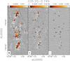 |
Fig. 1 VLA map of the 2 cm a), 1.3 cm b), and 7 mm c) continuum emission of G35.20N observed in B configuration. The VLA synthesized beam is shown in the lower left corner of each panel. The contours are 3, 6, 9, 18, 27, 36, and 45 times 1σ, which is 0.033 mJy beam-1, for a) and b), and 3, 18, and 54 times 1σ, which is 0.04 mJy beam-1, for c). The numbers correspond to the centimeter continuum sources detected (see Table 2). |
Continuum images at 6 and 3.6 cm in the A configuration were obtained from the VLA archive (project AG0576). The observations were carried out on September 15, 1999, with phase center α(J2000) = 18h58m1293, δ(J2000) = + 01°40′365. The final maps have been reprojected to the phase center of our VLA observations. The data were re-calibrated and imaged with CASA to create maps with the same Briggs robustness parameter as the 2 and 1.3 cm and 7 mm maps. The maps and the fluxes are very similar to those obtained by Gibb et al. (2003) with uniform weighting.
2.2. VERA observations
VLBI Exploration of Radio Astrometry (VERA) observations of the H2O maser line at 22.235 GHz were carried out on September 06, October 10, November 05, December 03, 2013, and January 10, 2014. All four stations of VERA were used in all sessions, providing a maximum baseline length of 2270 km. Observations were made in the dual beam phase-referencing mode; G35.20N and a reference source J1858+0313 (α(J2000) = 18h58m02352576, δ(J2000) = +03°13′1630172) were observed simultaneously with the separation angle of 1.55°. The instrumental phase difference between the two beams was measured continuously during the observations by injecting artificial noise sources into both beams at each station (Honma et al. 2008a).
The data were recorded onto magnetic tapes sampled with 2-bit quantization at a rate of 1024 Mbps. Among a total bandwidth of 256 MHz, one IF channel and the rest of 15 IF channels with a 16 MHz bandwidth each were assigned to G35.20N and J1858+0313, respectively. A bright extragalactic radio source, J1743-0350, was observed every 80 min as a delay and bandpass calibrator.
Correlation processing was carried out on the Mitaka FX correlator located at the NAOJ Mitaka campus. For the H2O maser line, the spectral resolution was set to be 15.625 kHz, corresponding to the velocity resolution of 0.21 km s-1.
Data reduction was performed using the NRAO AIPS. First, results of the dual-beam phase calibration and the correction for the approximate delay model adopted in the correlation processing were applied to the visibility data (Honma et al. 2008b). Next, instrumental delays and phase offsets among all of the IF channels were removed by the AIPS task FRING on J1743-0350. Finally, residual phases were calibrated by the AIPS task FRING on J1858+0313. These FRING solutions were applied to the target source G35.20N. Synthesis imaging and deconvolution (CLEAN) were performed using the AIPS task IMAGR. The uniform weighted synthesized beam size (FWMH) was typically 1.5 mas × 0.8 mas with a position angle of −40°. The peak positions and flux densities of maser features were derived by fitting elliptical Gaussian brightness distributions to each spectral channel map using the AIPS task SAD.
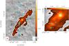 |
Fig. 2 (Left panel) Overlay of the ALMA 870 μm continuum emission (colors and red contours) from Sánchez-Monge et al. (2013) on the VLA 1.3 cm continuum emission (cyan contours) observed in B configuration. The cyan cross indicates the position of source 2, not detected at 1.3 cm, as estimated from the 2 cm map. The ALMA and VLA synthesized beam are shown in the lower left and lower right corner, respectively. Red contours are 5, 10, 15, 25, 50, and 100 times 1σ, which is 1.8 mJy beam-1. Cyan contours are the same as in Fig. 1. (Right panel) Close-up of the central region around cores A and B that shows the ALMA 870 μm continuum emission image overlaid with the VLA 1.3 cm continuum emission (cyan contours) observed in A configuration. Cyan contours are 3, 6, 18, 36, and 54 times 1σ, which is 0.023 mJy beam-1. Red contours are the same as in the left panel. The VLA synthesized beam is shown in the lower right corner. The numbers correspond to the centimeter continuum sources in Table 3. |
3. Results
3.1. Continuum emission
Figure 1 shows the maps of the continuum emission at 2 and 1.3 cm, and 7 mm towards G35.20N observed in the B configuration with the VLA. A total of 16 sources have been detected in at least one wavelength. The positions of the sources and their peak intensities and integrated flux densities estimated in the B and A configuration are given in Tables 2 and 3, respectively. For comparison, the tables also indicate the number assigned by Gibb et al. (2003) to the radio sources. Because there are far fewer sources detected at 6 and 3.6 cm than we detected at 2 cm, 1.3 cm, and 7 mm, we preferred to re-number the radio sources ordering them by increasing right ascension. Table 3 gives also the peak intensity and integrated flux density at 6 and 3.6 cm.
Position, peak intensity, and integrated flux density of the cores estimated from the B-array images.
Peak intensity and flux density of the cores estimated from the A-array images.
Source 2 shows a peculiar behavior at 1.3 cm because it is clearly detected in the A configuration (see Table 3) but not in the B configuration (its intensity is <0.1 mJy beam-1, a factor ~2.2 lower than in the A configuration). A possible explanation could be source variability. In this case the timescales for this variability should be very short (1.5 months), but Hofner et al. (2007) have reported strong variability on timescales of only one day for the source I20var in IRAS 20126+4104.
As seen in Tables 2 and 3, sources 10, 11, 12, and 15 are unresolved at 1.3 cm and 7 mm in the B configuration, as indicated by the fact that their peak and integrated flux density at 1.3 cm are the same. These sources are not detected in the A configuration, even though the sensitivity is better. This implies that the source angular diameters are smaller than the synthesized beam ( ) of the B configuration, but are partially resolved in the A configuration image. The latter condition sets a lower limit to the angular diameters which are, respectively,
  (source 10),
  (source 11), (source 12), and
  (source 15).
Most of the radio sources are distributed in a N–S direction that roughly coincides with that of the wall of the cavity of the NE–SW molecular outflow mapped in CO (3–2) by Gibb et al. (2003) and in CO (7–6) by Qiu et al. (2013). Based on the distribution of the radio sources, Gibb et al. (2003) conclude that these sources trace a precessing thermal radio jet and that such a radio jet is not driving the large-scale molecular outflow. The sources likely associated with this N–S radio jet show an extended morphology, with the exception of those located close to the geometrical center (sources 6, 8, and 9), which have a more compact structure. One of these compact sources, source 8 (resolved into 8a and 8b in the 1.3 cm and 7 mm maps), is associated with core B (Fig. 2), the Keplerian disk candidate associated with a B-type (proto)star identified by Sánchez-Monge et al. (2013). As seen in Figs. 1b and c and 2, the centimeter emission of core B is resolved into two sources at all wavelengths but 2 cm. Along the N–S structure, there is one source (14) that has only been detected at 2 cm (at a 9σ level). Gibb et al. (2003) have detected a source at 6 cm at α(J2000) = 18h58m1307, δ(J2000) = +01°40′401 (source 4 in their notation) that is not visible at any other wavelength. However, this source is detected at a 3σ level, which casts some doubts on the reliability of the detection.
Figure 1 also shows a group of three sources (1, 3, and 10) roughly aligned in the NE–SW direction. The morphology of these sources, in particular sources 1 and 3, is very compact at all wavelengths. These three sources could be associated with the SiO high-velocity emission observed by Gibb et al. (2003) and Sánchez-Monge et al. (2014), which could be tracing a second thermal radio jet. One of these three radio sources (3) is associated with core A (Fig. 2), the other hot molecular core in G35.20N that shows a velocity gradient suggestive of rotation (Sánchez-Monge et al. 2014). This source is clearly seen at 1.3 cm and 7 mm but only barely detected at 2 cm.
Finally, radio source 2 does not seem to be associated with any of the (putative) outflows in the regions nor with dust continuum emission (Fig. 2). This source is very compact and visible at 2 cm in the B configuration and at 1.3 cm and 7 mm in the A configuration. The source has also been detected at 6 and 3.6 cm by Gibb et al. (2003) (see Table 3).
Parameters of the Class I 44 GHz CH3OH maser features.
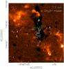 |
Fig. 3 H2 2.12 μm emission towards G35.20N from the UWISH2 survey (Froebrich et al. 2011) overlaid by the 1.3 cm continuum emission (cyan contours) observed in the B configuration. Cyan contours are the same as in Fig. 1. The numbers and white crosses indicate the positions of the Class I 44 GHz CH3OH masers (see Table 4). Green crosses mark the positions of the 870 μm continuum sources core A and B (Sánchez-Monge et al. 2014). |
3.2. CH3OH masers at 44 GHz
Class I methanol masers are usually associated with high-mass star-forming regions. Unlike the most common and bright Class II methanol masers that are radiatively pumped (e.g., Sobolev 2007, and references therein), Class I masers are collisionally pumped and could be associated with molecular outflows (Plambeck & Menten 1990; Voronkov et al. 2006). Our VLA observations at 44 GHz have revealed the presence of Class I CH3OH maser emission in G35.20N. The presence of 44 GHz CH3OH maser emission in G35.20N had been previously reported by Val’tts & Larionov (2007), but the positions of the maser spots had never been published before. A total of 14 maser spots have been detected in both configurations, A and B. Their positions, peak intensities, and velocity ranges are given in Table 4. Unfortunately, the limited spectral resolution of the observations (~7 km s-1) was not enough to separate the different spectral components. In fact, except for one maser spot that has only been detected in one spectral channel and two that have been detected in two spectral channels, the rest have been detected in three spectral channels covering a velocity range of 21 km s-1. This suggests that most of the maser emission that we observed is made of multiple velocity components. One of the spots, number 4, has an elongated morphology in the B configuration and is barely resolved into two components in the A configuration.
Figure 3 shows an image of the H2 emission towards G35.20N overlaid by the 1.3 cm continuum emission observed in the B configuration and the positions of the 44 GHz methanol masers. Almost all of the masers are located to the south of core B and seem to follow the distribution of the centimeter continuum sources and lie on the redshifted lobe of the CO outflow observed by Gibb et al. (2003) and Qiu et al. (2013). This suggests that the maser spots could trace the walls of the cavity excavated by the outflow, outlined by the H2 emission (Fig. 3). The only maser spots that could be associated with the NE blueshifted lobe are numbers 13 and 14. There are also three maser spots, numbers 2, 3, and 14 located to the west and east of cores A and B. These masers could be associated with the walls of the lobes of the CO outflow. Alternatively, these maser spots could be tracing a second flow directed E–W and associated with the centimeter sources 1, 3, and 10, as suggested in the previous section.
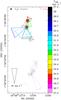 |
Fig. 4 Distribution of water masers (colored triangles) towards G35.20N overlaid with the 1.3 cm (grayscale image) and 7 mm (red contours) VLA continuum observed in the B configuration. Colored triangles show the absolute position of individual maser features, with colors denoting the maser VLSR according to the color-velocity conversion code shown on the right side of the panel. The triangle area is proportional to the logarithm of the maser intensity. Colored cones represent the measured maser proper motions, with cone aperture giving the uncertainty on the direction of the motion. The amplitude scale for the maser velocity is indicated by the black cone at the bottom left of the panel. The grayscale image reproduces linearly the intensity of the VLA B-Array 1.3 cm continuum from 0.05 mJy beam-1 (≈3σ) to 1.7 mJy beam-1. The red contours reproduce the B-Array 7 mm continuum, plotting levels from 10% to 90%, in steps of 10%, of the peak value of 3.5 mJy beam-1. Radio knots are labeled using the same numbers as in Table 2. |
3.3. H2O masers
Water masers are typically associated with winds/jets from both low- and high-mass YSOs. They are thought to be collisionally excited in relatively slow (≤ 30 km s-1) C-shocks and/or fast (≥ 30 km s-1) J-shocks (Gray 2012; Hollenbach et al. 2013) produced by the interaction of the protostellar outflow with very dense (nH2≥ 107 cm-3) circumstellar material. Water maser emission towards G35.20N was previously observed with the VLA (see, e.g., Codella et al. 2010), but to our knowledge no Very Long Baseline Interferometry (VLBI) observations of the 22 GHz masers towards this source have been reported in the literature. Figure 4 reports absolute positions and velocities of the water maser features detected with our VERA observations. For a description of the criteria used to identify individual masing clouds, to derive their parameters (position, intensity, flux, and size), and to measure their proper motions (relative and absolute), see the paper on VLBI observations of water and methanol masers by Sanna et al. (2010). The derived absolute water maser proper motions were corrected for the apparent proper motion due to the Earth’s orbit around the Sun (parallax), the solar motion, and the differential Galactic rotation between our LSR and that of the maser source. We have adopted a flat Galaxy rotation curve (R0 = 8.33 ± 0.16 kpc, Θ0 = 243 ± 6 km s-1) (Reid et al. 2014) and the solar motion ( ,
,  , and
, and  km s-1) by Schönrich et al. (2010), who recently revised the Hipparcos satellite results.
Table 5 reports the parameters of the twelve detected maser features. Water maser emission extends N–S across ≈5.̋6 with a close spatial correspondence with the central portion of the radio jet. In fact, most of the maser features are observed near the radio knots 8a, 9, and 5. Maser proper motions are mainly pointing to the south with amplitudes in the range 10–50 km s-1, that apparently increase from north to south.
22.2 GHz H2O maser parameters for G35.20−0.74N.
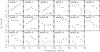 |
Fig. 5 Continuum spectra for the centimeter continuum sources. Circles and upper limits correspond to the observational data from Tables 2 and 3. For sources 1, 3, and 8a the dotted line indicates the linear fit (Sν ∝ να) from 6 cm to 7 mm (for source 3 the fit was done from 3.6 cm to 7 mm). |
4. Analysis
4.1. Continuum spectra
Figure 5 shows the continuum spectra for all the centimeter sources detected in at least one wavelength. The spectra have been estimated with the fluxes tabulated in Tables 2 and 3. For most of the sources the emission is so compact at all wavelengths and angular resolutions that the integrated fluxes hardly change when the maps are re-constructed with the same uvrange and restoring beam. As seen in this figure, only three sources (1, 3, and 8a) have spectral index α> 1 (assuming Sν ∝ να). For source 7, without taking into account the emission at 7 mm, α ≃ 0 is consistent with optically thin free-free (α = −0.1) emission. This source has a flux density at 7 mm of 0.19 mJy in the B configuration, but it is not detected at a 3σ level of 0.10 mJy in the A configuration. A possible explanation for such a faint emission at 7 mm, as compared to the emission at the other wavelengths, could be that the source is very extended and its emission has almost been resolved out by the interferometer. This is supported by the fact that the source is barely detected at 1.3 cm and is not detected at 7 mm at the higher angular resolution provided by the A configuration. Source 8b has a spectral index α ≃ −0.2, which is also consistent with optically thin free-free emission. The emission of this source at some wavelengths is very weak and very difficult to separate from the stronger emission of 8a. In fact, at 2 cm it has not been possible to estimate it. Therefore, the flux density estimates are more uncertain.
For most of the sources, the emission shows a negative spectral index for wavelengths shorter than 3.6 or 2 cm. For some of these, the continuum spectra shows a double slope, sharply increasing at longer wavelengths and then decreasing for shorter ones (e.g., source 2). A possible explanation for this behavior could be that the observations at 6 and 3.6 cm, carried out at a very different epoch (1999) than ours (2013–2014), had some calibration problems. However, this seems inconsistent with the fact that for some sources (e.g., 1 or 8a) the 6 and 3.6 cm fluxes are in agreement with the extrapolation of the fluxes at shorter wavelengths. Another possibility could be variability of the sources. Since the observations at longer and shorter wavelengths were separated by almost 15 yr, variability could affect the estimated fluxes and the spectral index determinations. In fact, as suggested in Sect. 3.1, source 2 could be variable. A strong variability is characteristic of extragalactic sources. Following Anglada et al. (1998), the expected number of background extragalactic sources at 1.3 cm within a field of diameter 2′ (the primary beam at 1.3 cm) is given by ⟨N⟩= , where S0 is the detectable flux density threshold at the center of the field in mJy. For S0 = 0.10 mJy (3σ in the B configuration), the expected number of background extragalactic sources is 0.07. A similar value is obtained at 6 cm using the same field and the same S0, which is also 3σ at 6 cm. Only using a field at 6 cm with a diameter
  , which is much larger than the field in which the radio sources have been detected, the expected number of background sources would be one.
This result is in agreement with the fact that most of the centimeter sources should be associated with the thermal radio jet. In principle, thermal sources should not have strong variability, so this could indicate that the emission of some of the knots of the radio jet is non-thermal. In particular, Rodríguez et al. (1989) measured a negative spectral index of α = −0.7 for the radio jet powered by the YSO S68 FIRS1, which has been interpreted as produced by non-thermal emission. More recently, Carrasco-González et al. (2010) have revealed synchrotron emission arising from the HH 80–81 jet. In fact, the presence of synchrotron emission in radio jets might be more common than originally expected, as has been shown by the recent results of Moscadelli et al. (2013, 2016). Therefore, non-thermal variable emission could be a plausible explanation for the negative spectral indexes and the strange continuum spectra obtained for most of the sources. In order to test the variability of the sources, new observations at 6 and 3.6 cm are needed.
Source 14 is the only one that has been detected at only one wavelength (2 cm) at a 9σ level. A possible explanation for the non-detection at 1.3 cm and 7 mm is that the source, which is slightly extended at 2 cm, has been resolved out by the interferometer at these wavelengths. Regarding the non-detection at 6 and 3.6 cm, the expected peak flux densities, estimated by extrapolating the peak flux density measured at 2 cm (0.28 mJy beam-1) with a spectral index of 1 and taking into account the size of the source and the different synthesized beams, are 0.11 and 0.05 mJy beam-1, respectively. These fluxes are similar to or below the 3σ level and are therefore consistent with the fact that source 14 has not been detected at these wavelengths.
In conclusion, most of the radio sources in G35.20N have spectral indices that are either negative (i.e., the flux decreases with frequency) or consistent with source variability. In both cases, the most likely explanation is that their emission is non-thermal. The only sources that have spectral indices consistent with free-free thermal emission from ionized gas are sources 3, 8a, and 8b associated with the hot molecular cores A and B (Figs. 2 and 6), and sources 1 and 7.
5. Discussion
The main goal of our high-angular resolution centimeter observations was to investigate the existence of a binary system at the center of the massive core B in G35.20N. Such a system could explain the mass of 18 M⊙, computed from the velocity field, and the possible precession of the radio jet. The latter is supported by the S-shaped morphology of the jet and by the jet position angle, which is very different from that of the CO outflow (e.g., Heaton & Little 1988; Gibb et al. 2003). Another feature of the radio jet is that its expansion, suggested by the proper motions of the H2O masers (see Sect. 3.3), can also be estimated from the centimeter continuum emission at different epochs. All these issues will be discussed in detail in Sects. 5.2 to 5.4. In the next section we investigate the nature of the free-free emission of source 8a, associated with core B, and source 3, associated with core A. We also discuss the nature of source 1, which could be powering an additional jet in the region.
5.1. Origin of the free-free ionized gas emission
The only three sources that have a positive spectral index consistent with thermal emission from ionized gas are 1, 3, and 8a. Their spectral index is 1.1–1.3, consistent with partially optically thick emission arising from a thermal radio jet (e.g., Anglada 1996) or an ultracompact or hypercompact Hii (UC/HC Hii) region with a density gradient (e.g., Franco et al. 1990). In the following we discuss these two possibilities and explore the properties of the sources for each scenario.
5.1.1. Radio jet
Source 8a is located at the center of the N–S radio jet, first mapped by Gibb et al. (2003), while sources 3 and 1 lie at the center and edge, respectively, of what could be a second radio jet centered on core A (see Sánchez-Monge et al. 2014). Typical spectral indices of radio jets are α≲ 1.3 (Anglada 1996). Therefore, the emission of the three sources could be in fact arising from free-free thermal emission of radio jets. In this scenario the gas is ionized by the UV photons emitted by the shock at the interface between a neutral stellar wind and the surrounding high-density gas (Torrelles et al. 1985).
Reynolds (1986) modeled the emission of collimated, ionized stellar winds. According to this model, for a radio jet with constant velocity, temperature, and ionization fraction, the spectral index of the emission is related to its collimation through the expression α = 1.3−0.7/ϵ, where ϵ is the power-law index of the dependence of the jet radius on the distance from the central object. When the emission of the three sources arises from radio jets, its collimation ϵ would be >3.9 (Table 6). Therefore, these radio sources would have an increasing opening angle with distance from the star and would be poorly confined at the small scales of a few hundreds of au at which the centimeter observations are sensitive. The model of Reynolds (1986) also estimates the injection radius r0, i.e., the distance at which the ionized flow originates, assuming an isothermal radio jet. This distance determines the turnover frequency νm above which the entire jet becomes optically thin. Following Eq. (1) of Beltrán et al. (2001), we estimated r0 from the 1.3 cm B configuration data assuming an electron temperature T = 104 K and θ0 = 1 rad and sini = 1, where θ0 is the jet injection opening angle and i is the jet axis inclination with respect to the line of sight. The assumption sini = 1 implies that the jet lies on the plane of the sky and in some particular cases this can produce a significant underestimate of the injection radius r0. However, for a random orientation of the jet in space, the average value of sini is π/ 4, which changes the r0 estimate only by 13%. The assumption θ0 = 1 rad implies that the jet is poorly collimated (according to Reynolds 1986, well-collimated jets have θ0 ≲ 0.5), in agreement with what is suggested by the collimation parameter ϵ. Figure 5 shows that there is no hint of turnover in the spectra of sources 8a, 3, and 1. Therefore, we assumed 43.94 GHz (λ= 7 mm) to be a lower limit to the turnover frequency and estimated an upper limit for the injection radius. The values of r0 obtained are 50–90 au (Table 6), indicating that the ionization of the jet begins at a small distance from the star.
The model of Reynolds (1986) also allows us to estimate the ionized mass-loss rate in the jet Ṁion. Following Eq. (3) of Beltrán et al. (2001), we estimated Ṁion for a pure hydrogen jet, assuming a stellar wind velocity V⋆ of 200 km s-1, θ0 = 1 rad, and sini = 1. For a random orientation of the jet in space, the mass-loss rate in the jet would be underestimated only by 6%. The values of Ṁion are 1.4–3.2 ×10⁻⁶M⊙ yr-1 (Table 6). These values are consistent with the values of 10-6M⊙ yr-1 found by Ceccarelli et al. (1997) in low-mass Class 0 objects and are 2–3 orders of magnitude higher than those found by Beltrán et al. (2001) in more evolved low-mass young stellar objects. We note that these values have to be taken as lower limits, not only because the turnover frequency is a lower limit, but also because the stellar wind velocity could be higher for high-mass YSOs.
Parameters of the radio jets.
Physical parameters of the UC/HC Hii regions.
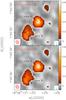 |
Fig. 6 (Top panel) Overlay of the 1.3 cm continuum emission (cyan contours) observed in A configuration on the average emission in the CH3CN (19–18) K = 2 line (colors and red contours) at 350 GHz observed with ALMA by Sánchez-Monge et al. (2013). The cyan contours are 3, 12, 30, and 54 times 1σ, which is 0.023 mJy beam-1. The velocity interval used to calculate the CH3CN mean emission is 25.9–33.0 km s-1. The red contour levels are 1, 2, 3, 5, 7, 10, and 15 times 50 mJy beam-1. The ALMA and VLA synthesized beams are shown in the lower left and lower right corner, respectively. The numbers correspond to the centimeter continuum sources in Table 3. (Bottom panel) Same for the 7 mm continuum emission. The cyan contours are 3, 12, and 48 times 1σ, which is 0.033 mJy beam-1. |
5.1.2. UC/HC HII region
The free-free emission of sources 1, 3, and 8a could also be explained in terms of photoionization. Thermal radio jets are expected to have an extended and elongated morphology at subarcsecond angular resolution (e.g., Anglada 1996) and lower flux at higher angular resolution because part of the extended emission is filtered out by the interferometer. In fact, the typical sizes (a few 100 au) of radio jets associated with high-mass protostars (e.g., Anglada et al. 2014) should be easily resolved at the angular resolution of ~ (~100 au at the distance of G35.20N) reached at 7 mm in the A configuration. In contrast, the observations of Gibb et al. (2003), with a maximum angular resolution of ~
 at 3.6 cm, were not able to properly resolve the emission and distinguish between a radio jet or an UC/HC Hii region origin. As seen in Fig. 6, none of the three free-free sources is resolved. On the contrary, the sources are very compact and their fluxes do not change from the B to the A configuration. Furthermore, two of the free-free sources, 3 and 8a, are associated respectively with the hot molecular cores A and B (see Fig. 6). This also favors the interpretation of the emission as being due to photoionization because hot cores are often known to be associated with UC/HC Hii regions.
Assuming that the centimeter continuum emission comes from homogeneous optically thin UC/HC Hii regions, we used the data at 1.3 cm obtained with the B configuration to calculate the physical parameters of the three sources (using the equations of Mezger & Henderson 1967 and Rubin 1968; see also the Appendix of Schmiedeke et al. 2016). Table 7 gives the spatial radius R of the UC/HC Hii region obtained from the deconvolved source size, the source averaged brightness TB, the electron density ne, the emission measure EM, the number of Lyman-continuum photons per second NLy, the mass of ionized gas Mion, calculated assuming a spherical homogeneous distribution, and the spectral type of the ionizing star. The last was computed from the estimated NLy using the tables of Davies et al. (2011) and Mottram et al. (2011) for zero age main sequence (ZAMS) stars.
As seen in Table 7, sources 1, 3, and 8a are ionized by stars of spectral type B1–B2, with masses of 8–11 M⊙ (Mottram et al. 2011). However, it has to be taken into account that the parameters of the UC/HC Hii regions have been estimated assuming optically thin emission while the spectral indices >1.1 indicate that the emission is partially optically thick. In this case, NLy, and therefore, the spectral type and the mass of the central objects, should be considered lower limits.
If source 8a is indeed an UC/HC Hii region and at the same time is the driving source of the radio jet (as suggested by its location at the geometrical center of the jet), then G35.20−0.74N would represent a unique example of a radio jet coexisting with an UC/HC Hii region powered by the same YSO. This suggests that this object is in a transitional stage between the main accretion phase, dominated by infall and ejection of material, and the phase in which the radiation pressure of the ionized circumstellar material overcomes infall and the newly formed UC/HC Hii region begins to expand (see Keto 2002). Guzmán et al. (2016) have very recently reported a similar case for G345.4938+01.4677. A similar scenario could be also valid for source 3, but in this case the existence of a radio jet is less clear. In this scenario, one of the knots of the jet would be source 1, but as discussed above, this centimeter source could also be an UC/HC Hii region; in fact, Fuller et al. (2001) propose source 1 as the driving source of an additional jet in the region, observed at near-infrared wavelengths. However, the association of source 3 with a dense core with signs of rotation would favor it as the driving source of the possible jet.
Based on the compact morphology of sources 1, 3, and 8a, which are not resolved even at a spatial resolution of ~100 au, and the poor collimation of the emission, we conclude that the most likely origin of their free-free emission is photoionization. Therefore, we believe that the three sources are likely associated with UC/HC Hii regions.
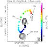 |
Fig. 7 VLA map of the 1.3 cm continuum emission (contours) towards G35.20N overlaid on the Keplerian disk traced by the peaks of the CH3CN(19–18) K = 2 emission at different velocities (solid circles, color-coded as indicated in the figure), imaged with ALMA (see Sánchez-Monge et al. 2013). The cross marks the position of the sub-mm continuum emission at 350 GHz. Contour levels range in logarithmic steps from 0.06 to 1.452 mJy/beam. The synthesized beam of the VLA is shown at the bottom right. |
5.2. Binary system in core B
Sánchez-Monge et al. (2013) observed G35.20N with ALMA at 870 μm and discovered a Keplerian rotating disk associated with core B. The best-fit model to the velocity field gives a mass of the central star of 18 M⊙. However, this poses a problem because the luminosity expected of such a massive star would be comparable to (or higher than, depending on the models used to estimate it) the luminosity of the whole star-forming region (3 × 10⁴ L⊙). Taking into account that the star-forming region is associated with at least one other hot molecular core (core A), it is unlikely that its luminosity is only produced by core B. This problem could be solved if the luminosity of the region has been underestimated because part of the stellar radiation escapes through the outflow cavities (Zhang et al. 2013). Alternatively, the existence of a binary system associated with core B could also be a solution (Sánchez-Monge et al. 2013) because in this case, the total luminosity of the members of the system could be significantly lower than that of the whole star-forming region.
Our high-angular resolution 1.3 cm and 7 mm observations appear to support the second scenario because we have resolved the centimeter emission associated with core B and confirmed the existence of a binary system by revealing two radio sources, 8a and 8b (see Fig. 7). The separation of the two sources is ~ , which corresponds to ~800 au at the distance of the region. Typical binary separations for T Tauri stars closely associated with early-type stars is 90 au (Brandner & Koehler 1998). However, massive stars have companions with larger separations, in the range of 103 to several 104 au (Sana & Evans 2011, and references therein).
Source 8a is the strongest of the pair and could be the one associated with the hot molecular core. Moreover, this source, as shown in Fig. 6, is located closer to the center of the hot molecular core seen in CH3CN. If we assume that the free-free emission of source 8a is due to an UC/HC Hii region, then its spectral type would be B1 and its mass should be ≳11 M⊙, as discussed in Sect. 5.1. The expected luminosity for a B1 star is ~6.3 ×10³ L⊙. In order to account for the 18 M⊙ estimated by Sánchez-Monge et al. (2013) from the velocity field of the disk, source 8b should have a mass ≲ 8 M⊙. The shape of the continuum spectrum of this source (Fig. 5), although uncertain, suggests that the emission could be consistent with optically thin free-free emission (see Sect. 4.1). Therefore, we decided to estimate the spectral type from the 1.3 cm observations in the A configuration (because the emission of source 8b is resolved from that of 8a) assuming that the centimeter emission arises from an optically thin UC/HC Hii region (see Table 7). The spectral type of source 8b would be B3, which corresponds to a ~6 M⊙ star with a luminosity of ~103 L⊙. This implies that the total mass of the binary system is ≳17 M⊙ in agreement with the stellar mass estimated from the velocity field, while its luminosity is ~7 ×10³ L⊙, lower than ~3 ×10⁴ L⊙, the luminosity of the whole star-forming region.
In conclusion, our observations have revealed the presence of a binary system of UC/HC Hii regions at the center of a Keplerian rotating disk in G35.20N (Fig. 7). The existence of a binary system solves the luminosity problem raised by Sánchez-Monge et al. (2013), without invoking the “flashlight effect” as suggested by Zhang et al. (2013). In this scenario, the Keplerian disk discovered by Sánchez-Monge et al. (2013) would indeed be a circumbinary disk, analogous to that observed in the young low-mass binary system GG Tau (e.g., Skrutskie et al. 1993). This close association of the young binary system with a Keplerian disk is suggestive of a scenario where the secondary 6 M⊙ star source 8b has formed from disk instabilities in an accretion disk around source 8a, which was initially massive enough to become non-axisymmetric. The mass ratio (the secondary to the primary) of this binary system is ~0.54. Three-dimensional radiation-hydrodynamic simulations by Krumholz et al. (2009) demonstrate the formation of secondary massive stars arising from disk instabilites with an initial mass ratio >0.5. This is a result of the SWING mechanism in nearly Keplerian disks, described by Adams et al. (1989) and then simulated by Laughlin & Bodenheimer (1994).
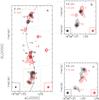 |
Fig. 8 a) Overlay of the 2 cm continuum emission (red contours) observed in B configuration on the 6 cm continuum emission (grayscale) in A configuration from Gibb et al. (2003). Red contours are the same as in Fig. 1a. The grayscale levels are 1, 2, 3, and 6 times 0.1 mJy beam-1, the 3σ level of the map. The VLA 6 and 2 cm synthesized beam are shown in the lower left and lower right corner, respectively. The numbers correspond to the centimeter continuum sources in Table 3. The black dashed line indicates the possible trajectory of the wiggling jet. b) and c) Overlay of the 1.3 cm continuum emission (red contours) observed in B configuration on the 3.6 cm continuum emission (grayscale) in A configuration from Gibb et al. (2003). Red contours are the same as in Fig. 1b. The grayscale levels are 1, 2, 3, and 4 times 0.08 mJy beam-1, the 3σ level of the map. The VLA 3.6 and 1.3 cm synthesized beam are shown in the lower left and lower right corner, respectively. |
5.3. Expansion of the radio jet
Figure 8 shows the comparison of the radio jet emission at two different epochs, 1999 and 2013. The former is the epoch of the Gibb et al. (2003) observations and the latter is that of our observations. This figure suggests that the radio jet is expanding. In fact, it shows that the radio knots at the northern and southern ends of the jet appear to have moved outward with time because the emission of the knots observed more recently, in particular at 1.3 cm, is located ahead of the emission of those observed by Gibb et al. (2003) at 6 and 3.6 cm. Vice versa, the position and compact morphology of the central radio sources have not changed significantly with time, consistent with the fact that they are UC/HC Hii regions. We note that some of the southern knots show slightly transverse motions with respect to the direction of the jet (Fig. 8c), similar to what has been observed towards the radio jet in IRAS 16547−4247 (Rodríguez et al. 2008).
The difference between the old and the new positions of the knots is ~ for source 7 in the north, and
  – for sources 4 and 5 in the south. These angular separations correspond to ~880 au and 440–550 au, respectively. For a time lapse of 14 yr, the separation of the knots would indicate a velocity of the jet on the plane of the sky of 150–300 km s-1, consistent with the proper motions measured for low-mass radio jets (e.g., Anglada 1996). Because these velocities are on the plane of the sky, the real speeds may be higher. The proper motions of the H2O masers observed southward of source 8a also suggest that the jet is expanding. In particular, the southernmost redshifted maser spot is expanding in the same direction as that suggested by the free-free emission, namely S–SW. However, the velocities of expansion inferred from the centimeter continuum emission and the maser emission are different. The 3D velocities of the masers, ≲ 50 km s-1, are much lower than the expansion velocities, which are 150–300 km s-1 (at least), estimated from the radio jet emission. This is especially evident at the southern position where the maser emission coincides with the free-free knot 5. Here the expansion velocity of the jet (150–190 km s-1) is 3–4 times higher than the speed of the H2O maser spot.
Since both the free-free and maser emissions originate in shocks produced in the interaction of the protostellar jet with circumstellar ambient material, the much lower velocities of the water masers can be explained in terms of the very high (nH2≥ 107 cm-3) pre-shock density required to produce maser emission. In fact, assuming that all the momentum of the jet is transferred to the shocked gas, it follows that, for a relatively light jet, the shock velocity depends inversely on the square root of the density of the ambient material (see, e.g., Masson & Chernin 1993). Based on the ratio of proper motion amplitudes of the radio knots and the water masers, we can infer that the ionized gas emission should trace the interaction of the jet with gas parcels about one order of magnitude less dense (i.e., nH2~ 106 cm-3) than those responsible for the water maser emission.
5.4. Precession of the radio jet
As can see in Fig. 8, the radio jet presents an S-shaped morphology, which is strongly suggestive of precession, as has been found in the case of other similar jets associated with low- and high-mass YSOs (e.g., HH–30: Anglada et al. 2007; IRAS 20126+4104: Shepherd et al. 2000; Cesaroni et al. 2005). Precession is often due to the interaction between the disk around the YSO powering the jet and a nearby stellar companion.
This provides us with the opportunity to tie the properties of the precessing jet to the parameters of the binary system. On the one hand, this equation (from Shepherd et al. 2000 and Terquem et al. 1999) 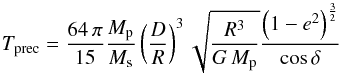 (1)can be used to express the precession period, Tprec, as a function of the masses of the primary (Mp) and secondary (Ms) members of the binary, the radius of the disk (R), the separation of the two stars (D), the eccentricity of the orbit (e), and the inclination of the binary orbit with respect to the plane of the disk (δ). On the other hand, Tprec can also be obtained from the ratio between the wavelength (λ) of the sinusoidal-like pattern of the jet and the jet expansion velocity (vjet):
  (2)By combining Eqs. (1) and (2), the following expression for λ is obtained:
  (3)This can be used to set a lower limit on λ. In fact, the masses of the two stars are Mp ≃ 11 M⊙ and Ms ≃ 6 M⊙ (see Sect. 5.2), while the projected separation on the plane of the sky between the two HC/UC Hii regions 8a and 8b may be taken as a lower limit on D, i.e. D> 800 au. Moreover, vjet ≃ 200 km s-1 (see Sect. 5.3) and R ≤ D because the part of the disk affected by the companion lies inside its orbit. Finally, cosδ ≤ 1 and the eccentricity of the orbit is unlikely to be very large and we thus assume e< 0.9 (see Mathieu 1994; Mason et al. 1998). Taking all these values into account, we find λ> 0.45 pc.
A value that large indicates that the radio emission is tracing only a small fraction of the precession pattern, whose extent must exceed the region shown in Fig. 1. This finding is consistent with the scenario proposed by Sánchez-Monge et al. (2014). By complementing the radio maps with near-IR images of the 2.12 μm H2 line emission (see their Fig. 16), these authors propose that the precessing jet/outflow from G35.20N extends over a much larger region than that traced by the radio jet itself. According to their interpretation, the precession axis is not oriented N–S, but closer to a NE–SW direction, and the value of λ is higher than our previous estimate. From Figs. 15 and 16 of Sánchez-Monge et al. (2014), it is possible to roughly derive λ/ 2 ≃ 30″, i.e., λ ≃ 0.6 pc, consistent with the lower limit derived above.
In conclusion, the properties of the binary system appear to support precession of the jet with a relatively large precessing angle, about a precession axis directed approximately NE–SW, which is in agreement with the interpretation proposed by Sánchez-Monge et al. (2014).
6. Conclusions
We carried out VLA observations in the continuum at 2 and 1.3 cm, and 7 mm of the high-mass star-forming region G35.20N to study the origin of the free-free emission, to examine the binary system hypothesis required to solve the luminosity problem in this source (Sánchez-Monge et al. 2013), and to characterize the possible precession of the radio jet. The high angular resolution observations from 0.05′′ to 0.45′′ have allowed us to obtained a very detailed picture of the radio continuum emission in this region. The main results can be summarized as follows:
-
We have detected 17 radio continuum sources in the region, some of them previously detected in the observations of Gibb et al. (2003). The spectral indices of the emission of the different sources are consistent with variable emission for most of them. For 4 out of 17 sources, the free-free emission is consistent with ionized emission from UC/HC Hii regions.
-
The observations have revealed the presence of a binary system of UC/HC Hii regions at the geometrical center of the radio jet. This binary system, which is associated with the Keplerian rotating disk discovered by Sánchez-Monge et al. (2013), consists of two B-type stars of 11 and 6 M⊙. The existence of a binary system solves the luminosity problem raised by Sánchez-Monge et al. (2013) because the total luminosity of the system would be ~7×10³L⊙, much lower than the luminosity of the whole star-forming region. The presence of such a massive binary system is in agreement with the theoretical predictions of Krumholz et al. (2009), according to which the gravitational instabilities during the collapse would produce the fragmentation of the disk and the formation of such a system.
-
The 7 mm observations have detected 14 Class I CH3OH maser spots in the region, most of them lying along the N–S direction of the radio jet and a few located in a N–E direction, coinciding with IR emission. This suggests an association between the methanol masers and the jet, consistent with the fact that Class I methanol masers are collisionally pumped.
-
The S-shaped morphology of the jet has been successfully explained as being due to precession produced by the binary system located at its center. By tying the properties of the precessing jet to those of the binary system, we have set a lower limit of ~0.45 pc on the typical wavelength of the S-shaped pattern. This proves that the precession extends over a larger region than that traced by the radio cm emission, consistent with a wide precession angle around the NE–SW direction, as proposed by Sánchez-Monge et al. (2014). In such a scenario, the three class I CH3OH maser spots located to the east and west could be tracing a second flow.
-
Comparison of the radio jet images obtained at 2 and 1.3 cm in 2013 with those obtained at 6 and 3.6 cm in 1999 (Gibb et al. 2003) suggests that the jet is expanding at a maximum speed on the plane of the sky of 300 km s-1. The proper motions of the H2O masers, detected in the region with the VERA interferometer, also indicate expansion in a direction similar to that of the radio jet.
The National Radio Astronomy Observatory is a facility of the National Science Foundation operated under cooperative agreement by Associated Universities, Inc.
The CASA package is available at http://casa.nrao.edu/
The GILDAS package is available at http://www.iram.fr/IRAMFR/GILDAS
Acknowledgments
We thank the referee, Andrés Guzmán, for his useful comments. We acknowledge a partial support from the Italian Foreign Minister (MAECI) as a project of major importance in the Scientific and Technological Collaboration between Italy and Japan.
References
- Adams, F. C., Ruden, S. P., & Shu, F. H. 1989, ApJ, 347, 959 [NASA ADS] [CrossRef] [Google Scholar]
- Anglada, G. 1996, in Radio emission from the stars and the sun, ASP Conf. Ser., 93, 3 [NASA ADS] [Google Scholar]
- Anglada, G., Villuendas, E., Estalella, R., et al. 1998, AJ, 116, 2953 [NASA ADS] [CrossRef] [Google Scholar]
- Anglada, G., López, R., Estalella, R., et al. 2007, AJ, 133, 2799 [NASA ADS] [CrossRef] [Google Scholar]
- Anglada, G., Rodríguez, L. F., & Carrasco-González, C. 2014, in Proc. Advancing Astrophysics with the Square Kilometre Array (AASKA14), 121 [Google Scholar]
- Beltrán, M. T., & de Wit, W. J. 2015, A&ARv, in press [Google Scholar]
- Beltrán, M. T., Estalella, R., Anglada, G., Rodríguez, L. F., & Torrelles, J. M. 2001, AJ, 121, 1556 [NASA ADS] [CrossRef] [Google Scholar]
- Bonnell, I. A., & Bate, M. R. 2006, MNRAS, 370, 488 [NASA ADS] [CrossRef] [Google Scholar]
- Brandner, W., & Koehler, R. 1998, ApJ, 499, L79 [NASA ADS] [CrossRef] [Google Scholar]
- Briggs, D. 1995, 1995, Ph.D. Thesis, New Mexico Inst. Mining & Tech. [Google Scholar]
- Carrasco-González, C., Rodríguez, L. F., Anglada, G., et al. 2010, Science, 330, 1209 [NASA ADS] [CrossRef] [PubMed] [Google Scholar]
- Ceccarelli, C., Haas, M. R., Hollenbach, D. J., & Rudolph, A. L. 1997, ApJ, 476, 771 [NASA ADS] [CrossRef] [Google Scholar]
- Cesaroni, R., Neri, R., Olmi, L., et al. 2005, A&A, 434, 1039 [NASA ADS] [CrossRef] [EDP Sciences] [Google Scholar]
- Codella, C., Cesaroni, R., López-Sepulcre, A., et al. 2010, A&A, 510, A86 [NASA ADS] [CrossRef] [EDP Sciences] [Google Scholar]
- Davies, B., Hoare, M., Lumsden, S. L. et al. 2011, MNRAS, 416, 972 [NASA ADS] [CrossRef] [Google Scholar]
- Franco, J., Tenorio-Tagle, G., & Bodenheimer, P. 1990, ApJ, 349, 126 [NASA ADS] [CrossRef] [Google Scholar]
- Foebrich, D., Davis, C. J., Ioannidis, G., et al. 2011, MNRAS, 413, 480 [NASA ADS] [CrossRef] [Google Scholar]
- Fuller, G. A., Zijlstra, A. A., & Williams, S. J. 2001, ApJ, 555, L125 [NASA ADS] [CrossRef] [Google Scholar]
- Gibb, A. G., Hoare, M. G., Little, L. T., & Wright, M. C. H. 2003, MNRAS, 339, 1011 [NASA ADS] [CrossRef] [Google Scholar]
- Gray, M. 2012, in Maser Sources in Astrophysics (Cambridge University Press) [Google Scholar]
- Guzmán, A., Garay, G., Brooks, K. J., Voronkov, M. A. 2012, ApJ, 753, 51 [NASA ADS] [CrossRef] [Google Scholar]
- Guzmán, A., Garay, G., Rodríguez, L. F. et al. 2016, ApJ, 826, 208 [NASA ADS] [CrossRef] [Google Scholar]
- Heaton, B. D., & Little, L. T. 1988, A&A, 195, 193 [NASA ADS] [Google Scholar]
- Hofner, P., Cesaroni, R., Olmi, L., et al. 2007, A&A, 465, 197 [NASA ADS] [CrossRef] [EDP Sciences] [Google Scholar]
- Hollenbach, D., Elitzur, M., & McKee, C. F. 2013, ApJ, 773, 70 [NASA ADS] [CrossRef] [Google Scholar]
- Honma, M. Kijima, M., Suda, H., et al. 2008a, PASJ, 60, 935 [NASA ADS] [CrossRef] [Google Scholar]
- Honma, M., Tamura, Y., & Reid, M. J. 2008b, PASJ, 60, 951 [NASA ADS] [Google Scholar]
- Keto, E. 2002, ApJ, 580, 980 [NASA ADS] [CrossRef] [Google Scholar]
- Keto, E. 2007, ApJ, 666, 976 [NASA ADS] [CrossRef] [Google Scholar]
- Krumholz, M. R., Klein, R. I., McKee, C. F., Offner, S. S. R., & Cunningham, A. J. 2009, Science, 323, 754 [NASA ADS] [CrossRef] [PubMed] [Google Scholar]
- Laughlin, G., & Bodenheimer, P. 1994, ApJ, 436, 335 [NASA ADS] [CrossRef] [Google Scholar]
- Masson, C. R., & Chernin, L. M. 1993, ApJ, 414, 230 [NASA ADS] [CrossRef] [Google Scholar]
- Mason, B. D., Gies, D. R., Hartkopf, W. I., et al. 1998, AJ, 115, 821 [NASA ADS] [CrossRef] [Google Scholar]
- Mathieu, R. D. 1994, ARA&A, 32, 465 [NASA ADS] [CrossRef] [Google Scholar]
- Mezger, P. G., & Henderson, A. P. 1967, ApJ, 147, 471 [NASA ADS] [CrossRef] [Google Scholar]
- Moscadelli, L., Cesaroni, R., Sánchez-Monge, Á., et al. 2013, A&A, 558, A145 [NASA ADS] [CrossRef] [EDP Sciences] [Google Scholar]
- Moscadelli, L., Sánchez-Monge, Á., Cesaroni, R., et al. 2016, A&A, 585, A71 [NASA ADS] [CrossRef] [EDP Sciences] [Google Scholar]
- Mottram, J. C., Hoare, M. G., Davies, B., et al. 2011, ApJ, 730, 33 [Google Scholar]
- Plambeck, R. L., & Menten, K. M. 1990, ApJ, 364, 555 [NASA ADS] [CrossRef] [Google Scholar]
- Qiu, K., Zhang, Q., Menten, K. M., Liu, H. B., & Tang, Y.-W. 2013, ApJ, 779, 182 [NASA ADS] [CrossRef] [Google Scholar]
- Reid, M. J., Menten, K. M. Brunthaler, A., et al. 2014, ApJ, 783, 130 [Google Scholar]
- Reynolds, S. P. 1986, ApJ, 304, 713 [NASA ADS] [CrossRef] [Google Scholar]
- Rodríguez, L. F., Curiel, S., Moran, J. M., et al. 1989, ApJ, 346, L85 [NASA ADS] [CrossRef] [Google Scholar]
- Rodríguez, L. F., Moran, J. M., Franco-Hernández, R., et al. 2008, ApJ, 135, 2370 [Google Scholar]
- Rubin, R. H. 1968, ApJ, 154, 391 [NASA ADS] [CrossRef] [Google Scholar]
- Sánchez-Monge, Á., Beltrán, M. T., Cesaroni, R., et al. 2014, A&A, 569, A11 [NASA ADS] [CrossRef] [EDP Sciences] [Google Scholar]
- Sana, H., & Evans, C. J. 2011, in Active OB stars: structure, evolution, mass loss, and critical limits, 474 [Google Scholar]
- Sánchez-Monge, Á., Cesaroni, R., Beltrán, M. T., et al. 2013, A&A, 552, L10 [NASA ADS] [CrossRef] [EDP Sciences] [Google Scholar]
- Sanna, A., Moscadelli, L., Cesaroni, R., et al. 2010, A&A, 517, A71 [NASA ADS] [CrossRef] [EDP Sciences] [Google Scholar]
- Schmiedeke, A., Schilke, P., Möller, Th., et al. 2016, A&A, 588, A143 [Google Scholar]
- Schönrich, R., Binney, J., & Dehnen, W. 2010, MNRAS, 403, 1829 [NASA ADS] [CrossRef] [Google Scholar]
- Shepherd, D. S., Yu, K. C., Bally, J., & Testi, L. 2000, ApJ, 535, 833 [Google Scholar]
- Shepherd, D. S., Claussen, M. J., & Kurtz, S. E. 2001, Science, 292, 1513 [NASA ADS] [CrossRef] [PubMed] [Google Scholar]
- Skrutskie, M. F., Snell, R. L., Strom, K. M., et al. 1993, ApJ, 409, 422 [NASA ADS] [CrossRef] [Google Scholar]
- Sobolev, A. M., Cragg, D. M., Ellingsen, S. P., et al. 2007, in Proc. International Astronomical Union, IAU Symp., 242, 81 [Google Scholar]
- Terquem, C., Eislöffel, J., Papaloizou, J. C. B., & Nelson, R. P. 1999, ApJ, 512, L131 [NASA ADS] [CrossRef] [EDP Sciences] [Google Scholar]
- Torrelles, J. M., Ho, P. T. P., Rodríguez, L. F., & Cantó, J. 1985, ApJ, 288, 595 [NASA ADS] [CrossRef] [Google Scholar]
- Val’tts, I. E., & Larionov, G. M. 2007, in Astron. Rep., 51, 519 [Google Scholar]
- Voronkov, M. A., Brooks, K. J., Sobolev, A. M., et al. 2006, MNRAS, 373, 411 [NASA ADS] [CrossRef] [Google Scholar]
- Zhang, B., Zheng, X. W., Reid, M. J., et al. 2009, ApJ, 693, 419 [NASA ADS] [CrossRef] [Google Scholar]
- Zhang, Y., Tan, J. C., De Buizer, J. M., et al. 2013, ApJ, 767, 58 [NASA ADS] [CrossRef] [Google Scholar]
All Tables
Position, peak intensity, and integrated flux density of the cores estimated from the B-array images.
All Figures
|
Fig. 1 VLA map of the 2 cm a), 1.3 cm b), and 7 mm c) continuum emission of G35.20N observed in B configuration. The VLA synthesized beam is shown in the lower left corner of each panel. The contours are 3, 6, 9, 18, 27, 36, and 45 times 1σ, which is 0.033 mJy beam-1, for a) and b), and 3, 18, and 54 times 1σ, which is 0.04 mJy beam-1, for c). The numbers correspond to the centimeter continuum sources detected (see Table 2). |
| In the text | |
|
Fig. 2 (Left panel) Overlay of the ALMA 870 μm continuum emission (colors and red contours) from Sánchez-Monge et al. (2013) on the VLA 1.3 cm continuum emission (cyan contours) observed in B configuration. The cyan cross indicates the position of source 2, not detected at 1.3 cm, as estimated from the 2 cm map. The ALMA and VLA synthesized beam are shown in the lower left and lower right corner, respectively. Red contours are 5, 10, 15, 25, 50, and 100 times 1σ, which is 1.8 mJy beam-1. Cyan contours are the same as in Fig. 1. (Right panel) Close-up of the central region around cores A and B that shows the ALMA 870 μm continuum emission image overlaid with the VLA 1.3 cm continuum emission (cyan contours) observed in A configuration. Cyan contours are 3, 6, 18, 36, and 54 times 1σ, which is 0.023 mJy beam-1. Red contours are the same as in the left panel. The VLA synthesized beam is shown in the lower right corner. The numbers correspond to the centimeter continuum sources in Table 3. |
| In the text | |
|
Fig. 3 H2 2.12 μm emission towards G35.20N from the UWISH2 survey (Froebrich et al. 2011) overlaid by the 1.3 cm continuum emission (cyan contours) observed in the B configuration. Cyan contours are the same as in Fig. 1. The numbers and white crosses indicate the positions of the Class I 44 GHz CH3OH masers (see Table 4). Green crosses mark the positions of the 870 μm continuum sources core A and B (Sánchez-Monge et al. 2014). |
| In the text | |
|
Fig. 4 Distribution of water masers (colored triangles) towards G35.20N overlaid with the 1.3 cm (grayscale image) and 7 mm (red contours) VLA continuum observed in the B configuration. Colored triangles show the absolute position of individual maser features, with colors denoting the maser VLSR according to the color-velocity conversion code shown on the right side of the panel. The triangle area is proportional to the logarithm of the maser intensity. Colored cones represent the measured maser proper motions, with cone aperture giving the uncertainty on the direction of the motion. The amplitude scale for the maser velocity is indicated by the black cone at the bottom left of the panel. The grayscale image reproduces linearly the intensity of the VLA B-Array 1.3 cm continuum from 0.05 mJy beam-1 (≈3σ) to 1.7 mJy beam-1. The red contours reproduce the B-Array 7 mm continuum, plotting levels from 10% to 90%, in steps of 10%, of the peak value of 3.5 mJy beam-1. Radio knots are labeled using the same numbers as in Table 2. |
| In the text | |
|
Fig. 5 Continuum spectra for the centimeter continuum sources. Circles and upper limits correspond to the observational data from Tables 2 and 3. For sources 1, 3, and 8a the dotted line indicates the linear fit (Sν ∝ να) from 6 cm to 7 mm (for source 3 the fit was done from 3.6 cm to 7 mm). |
| In the text | |
|
Fig. 6 (Top panel) Overlay of the 1.3 cm continuum emission (cyan contours) observed in A configuration on the average emission in the CH3CN (19–18) K = 2 line (colors and red contours) at 350 GHz observed with ALMA by Sánchez-Monge et al. (2013). The cyan contours are 3, 12, 30, and 54 times 1σ, which is 0.023 mJy beam-1. The velocity interval used to calculate the CH3CN mean emission is 25.9–33.0 km s-1. The red contour levels are 1, 2, 3, 5, 7, 10, and 15 times 50 mJy beam-1. The ALMA and VLA synthesized beams are shown in the lower left and lower right corner, respectively. The numbers correspond to the centimeter continuum sources in Table 3. (Bottom panel) Same for the 7 mm continuum emission. The cyan contours are 3, 12, and 48 times 1σ, which is 0.033 mJy beam-1. |
| In the text | |
|
Fig. 7 VLA map of the 1.3 cm continuum emission (contours) towards G35.20N overlaid on the Keplerian disk traced by the peaks of the CH3CN(19–18) K = 2 emission at different velocities (solid circles, color-coded as indicated in the figure), imaged with ALMA (see Sánchez-Monge et al. 2013). The cross marks the position of the sub-mm continuum emission at 350 GHz. Contour levels range in logarithmic steps from 0.06 to 1.452 mJy/beam. The synthesized beam of the VLA is shown at the bottom right. |
| In the text | |
|
Fig. 8 a) Overlay of the 2 cm continuum emission (red contours) observed in B configuration on the 6 cm continuum emission (grayscale) in A configuration from Gibb et al. (2003). Red contours are the same as in Fig. 1a. The grayscale levels are 1, 2, 3, and 6 times 0.1 mJy beam-1, the 3σ level of the map. The VLA 6 and 2 cm synthesized beam are shown in the lower left and lower right corner, respectively. The numbers correspond to the centimeter continuum sources in Table 3. The black dashed line indicates the possible trajectory of the wiggling jet. b) and c) Overlay of the 1.3 cm continuum emission (red contours) observed in B configuration on the 3.6 cm continuum emission (grayscale) in A configuration from Gibb et al. (2003). Red contours are the same as in Fig. 1b. The grayscale levels are 1, 2, 3, and 4 times 0.08 mJy beam-1, the 3σ level of the map. The VLA 3.6 and 1.3 cm synthesized beam are shown in the lower left and lower right corner, respectively. |
| In the text | |
Current usage metrics show cumulative count of Article Views (full-text article views including HTML views, PDF and ePub downloads, according to the available data) and Abstracts Views on Vision4Press platform.
Data correspond to usage on the plateform after 2015. The current usage metrics is available 48-96 hours after online publication and is updated daily on week days.
Initial download of the metrics may take a while.